Prediction of Protein Function and Functional Sites From Protein Sequences

DigitalCommons@USU

DigitalCommons@USU

All Graduate Theses and Dissertations Graduate Studies 5-2009

Prediction of Protein Function and Functional Sites From Protein

Prediction of Protein Function and Functional Sites From Protein

Sequences

Sequences

Jing Hu

Utah State University

Follow this and additional works at: https://digitalcommons.usu.edu/etd Part of the Biology Commons

Recommended Citation Recommended Citation

Hu, Jing, "Prediction of Protein Function and Functional Sites From Protein Sequences" (2009). All Graduate Theses and Dissertations. 292.

https://digitalcommons.usu.edu/etd/292 This Dissertation is brought to you for free and open access by the Graduate Studies at

DigitalCommons@USU. It has been accepted for inclusion in All Graduate Theses and Dissertations by an authorized administrator of DigitalCommons@USU. For more information, please contact

FROM PROTEIN SEQUENCES by

Jing Hu

A dissertation submitted in partial fulfillment of the requirements for the degree

of DOCTOR OF PHILOSOPHY in Computer Science Approved: _______________________ _______________________

Dr. Changhui Yan Dr. Donald H. Cooley

Major Professor Committee Member

_______________________ _______________________

Dr. Heng-Da Cheng Dr. Xiaojun Qi Committee Member Committee Member

_______________________ _______________________

Dr. John R. Stevens Dr. Byron R. Burnham

Committee Member Dean of Graduate Studies

UTAH STATE UNVIVERSITY Logan, Utah

Copyright © Jing Hu 2009 All Rights Reserved

ABSTRACT

Prediction of Protein Function and Functional Sites From Protein Sequences

by

Jing Hu, Doctor of Philosophy Utah State University, 2009 Major Professor: Dr. Changhui Yan

Department: Computer Science

High-throughput genomics projects have resulted in a rapid accumulation of protein sequences. Therefore, computational methods that can predict protein functions and functional sites efficiently and accurately are in high demand. In addition, prediction methods utilizing only sequence information are of particular interest because for most proteins, 3-dimensional structures are not available. However, there are several key challenges in developing methods for predicting protein function and functional sites. These challenges include the following: the construction of representative datasets to train and evaluate the method, the collection of features related to the protein functions, the selection of the most useful features, and the integration of selected features into suitable computational models. In this proposed study, we tackle these challenges by developing procedures for benchmark dataset construction and protein feature extraction, implementing efficient feature selection strategies, and developing effective machine learning algorithms for protein function and functional site predictions. We investigate

these challenges in three bioinformatics tasks: the discovery of transmembrane beta-barrel (TMB) proteins in gram-negative bacterial proteomes, the identification of deleterious non-synonymous single nucleotide polymorphisms (nsSNPs), and the identification of helix-turn-helix (HTH) motifs from protein sequence.

ACKNOWLEDGMENTS

I would like to thank Dr. Changhui Yan for his detailed direction and encouragement for the research in this dissertation. I would also like to thank my

committee members, Dr. Don Cooley, Dr. Heng-Da Cheng, Dr. Xiaojun Qi, and Dr. John Stevens, for their inspiration, continuous supervision, and valuable advice throughout the entire process.

I cordially give thanks to my family, friends, and colleagues for their

encouragement, moral support, and patience as I worked my way from writing the initial proposal to this final document. I could not have done it without all of you.

Finally, it should be noted that although I am not the principle author of the paper on which Chapter 4 is based, I conducted the majority of the research reported in Chapter 4. The research I did not participate in is not reported in said chapter.

CONTENTS Page ABSTRACT... iii ACKNOWLEDGMENTS ...v LIST OF TABLES... ix LIST OF FIGURES ...x CHAPTER 1 INTRODUCTION ...1

1.1 Machine Learning and Bioinformatics Problems... ...1

1.2 Goals of This Dissertation ...2

1.2.1 The Construction of Benchmark Datasets ...2

1.2.2 The Compilation of Sequence-based Features...3

1.2.3 The Feature Selection Process ...4

1.2.4 The Development of Appropriate Machine Learning Techniques ..9

2 DISCOVERY OF TRANSMEMBRANE BETA-BARREL PROTEINS IN GRAM-NEGATIVE BACTERIAL PROTEOMES...13

2.1 Background...13

2.1.1 The Importance of TMB Proteins...13

2.1.2 The Need for Computational Methods to Identify TMB Protein ..14

2.1.3 Current Methods for the Identification of TMB Proteins ...15

2.1.4 Current Methods to Predict the Topology of TMB Proteins ...20

2.1.5 Motivation of This Study...22

2.2 Materials and Methods...23

2.2.1 Datasets...23 2.2.2 Feature Set ...24 2.2.3 Five-Fold Cross-Validation ...26 2.2.4 K-NN Algorithm...26 2.2.5 Feature Selection...29 2.2.6 Performance Measurement ...31 2.3 Results...32

2.3.1 The Proposed K-NN Method’s Ability to Identify TMB Proteins 32 2.3.2 Including Homologous Sequence Information Improves the

Performance ...32

2.3.3 Further Improvement of the Prediction Performance by Feature Selection...33

2.3.4 Comparison with Predictions Solely Based on Similarity Search.33 2.3.5 Comparison with Other Prediction Methods ...34

2.3.6 A Web Server for the Prediction of TMB Proteins...37

2.3.7 Genome Scan ...37

2.4 Discussion...41

2.5 Conclusion ...43

2.6 Future Work...43

3 IDENTIFICATION OF DELETERIOUS NON-SYNONYMOUS SINGLE NUCLEOTIDE POLYMORPHISMS ...45

3.1 Background...45

3.1.1 Neutral or Deleterious nsSNPs ...45

3.1.2 Current Methods for the Identification of Deleterious nsSNPs ...46

3.1.3 Motivation of This Study...54

3.2 Materials and Methods...55

3.2.1 Datasets...55

3.2.2 Feature Set ...56

3.2.3 Decision Tree Algorithm ...61

3.2.4 Performance Measurement ...63

3.2.5 Cross-Validation and Independent Test...64

3.2.6 Feature Selection...65

3.3 Results...66

3.3.1 The Developed Method Identifies Deleterious nsSNPs...66

3.3.2 Analysis of Selected Features ...69

3.3.3 Comparisons with Previously Published Methods ...73

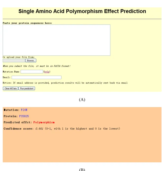
3.3.4 A Web Server for the Identification of Deleterious Non-synonymous Single Nucleotide Polymorphisms ...78

3.4 Discussion...78

3.5 Conclusion ...80

3.6 Future Work...80

4 IDENTIFICATION OF HELIX-TURN-HELIX MOTIFS FROM PROTEIN SEQUENCES ...83

4.1 Background...83

4.1.1 Helix-Turn-Helix: An Important Structure Through Which Proteins Bind with DNA...83

4.1.2 Current Prediction Methods to Identify Helix-Turn-Helix Motif..84

4.1.3 Motivation of This Study...91

4.2 Materials and Methods...92

4.2.1 Datasets...92

4.2.2 Hidden Markov Model...94

4.2.3 Feature Set ...98

4.2.4 Software Implementation...101

4.2.5 Performance Measurements...101

4.3 Results...101

4.3.1 Discretization of Solvent Accessibility...101

4.3.2 Constructing Profiles for Each HTH Protein Family Increases the Prediction Accuracy... 107

4.4 Discussion...112 4.5 Conclusion ...115 4.6 Future Work...116 5 CONCLUSION...117 REFERENCES ...120 VITA ...135

LIST OF TABLES

Table Page

1 Comparison of the Proposed K-NN Method with A Similarity Search. ... 34

2 Comparison of Different TMB Prediction Methods... 35

3 Prediction Results of 11 Gram-Bacteria Proteomes. ... 39

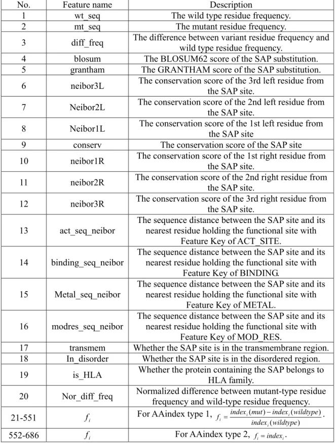
4 All Sequence-based Features of SAP Sites... 58

5 Prediction Performances of the Proposed Method... 68

6 List of Features in the Order They Are Selected. ... 68

7 Comparisons of Classification Methods of SAPs... 76

8 List of Reduced Alphabets... 100

9 HMM_AA_SA Achieves Better Performance Than HMM_AA by Dividing Solvent Accessibility into Two Discrete Categories. ... 104

10 HMM_AA_SA’s Performance Can Be Improved by Dividing Solvent Accessibility into Three Discrete Categories... 106

11 Including Solvent Accessibility Information into the Model and Using Reduced Alphabet Increase Performance in Identifying HTH Motifs. ... 109

LIST OF FIGURES

Figure Page

1 TMB proteins prediction web server ... 38

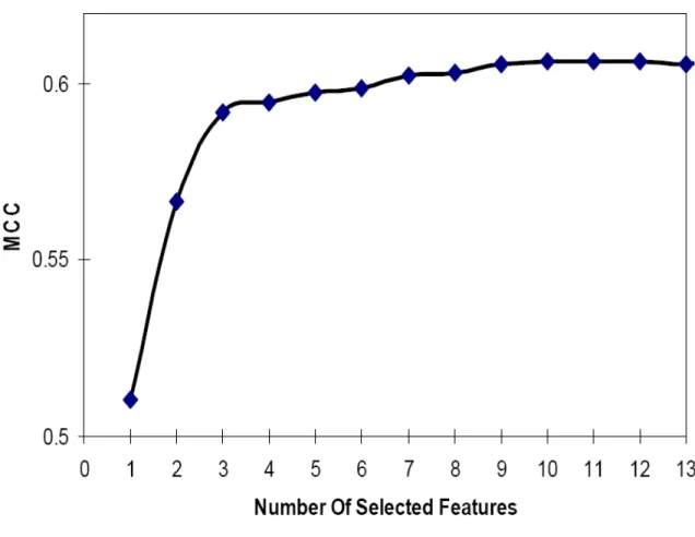
2 Classification performances as feature selection process progresses ... 67

3 Decision tree trained on 10 selected features as visualized using WEKA ... 71

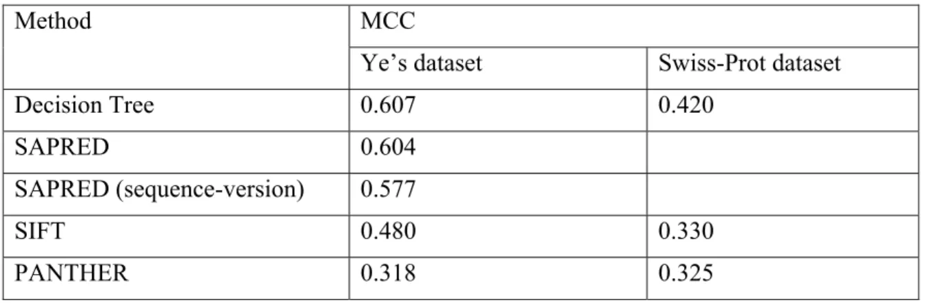
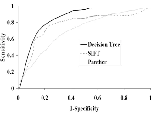
4 ROC curves of the proposed decision tree method, SIFT and PANTHER on Ye’s dataset... 77

5 ROC curves of the proposed decision tree method, SIFT and PANTHER on Swiss-Prot dataset ... 77

6 The web server for the prediction of deleterious SAPs ... 81

7 Images of HTH motifs ... 84

8 Hidden Markov model (right) that emits only amino acid residues ... 96

9 Hidden Markov model that emits both amino acids and solvent accessibility.. 97

10 The performance of HMM_AA_SA with solvent accessibility being divided into two categories ... 103

11 The performance of HMM_AA_SA with solvent accessibility being divided into three categories (α1, α2) with α1 = 0.05 ... 106

CHAPTER 1 INTRODUCTION

1.1 Machine Learning and Bioinformatics Problems

With the development of high-throughput genome sequencing projects in recent years, we have witnessed an exponential accumulation of biological data stored in public databases, i.e., DNA, RNA, and protein sequences. Because of their limitations and speed, experimental approaches can hardly keep up with the accumulation of new biological data. On the other hand, machine learning methods, which rely heavily on Bayesian probabilistic frameworks, are widely applied to learning knowledge and extracting information automatically from huge amount of biological data [1, 2, 3, 4].

Bioinformatics is a field that merges biology, computer science, and statistics into a single discipline.

Machine learning methods have achieved significant success in many

bioinformatics problems. For example, neural networks have been widely applied to predict protein secondary structure from amino acid sequences [5, 6, 7], to predict protein signal peptides and their cleavage sites [8, 9], to find genes in eukaryotic DNA, to

identify intron splice sites [10, 11], etc. Hidden Markov models have been proven to be useful in protein pair-wise sequence alignment [12, 13], multiple sequence alignment [14], protein homology detection [13, 15], protein structure prediction [16, 17], topology annotation for alpha-helical transmembrane proteins [18, 19], beta barrel proteins [20], and genomic annotation [21, 22], etc. Other machine learning techniques, such as support

vector machine, decision tree, random forest, k-nearest neighbor are also used to solve many bioinformatics problems.

1.2 Goals of This Dissertation

Numerous computational methods have been developed to predict protein function and functional sites by using information derived from protein sequences and structures. However, the 3-dimensional structural information of most proteins is not available, which limits the application of structure-based methods. Therefore,

computational methods that only require sequence information are key because they have a broader range of applications than structure-based methods.

In this study, we develop efficient machine-learning approaches to discover the attribute-class relationship between sequence features and protein functions. There are several challenges in constructing computational methods with high performance. These challenges include the topics discussed in Sections 1.21 through 1.24 below.

1.2.1 The Construction of Benchmark Datasets

In order to develop efficient and accurate computational methods, it is necessary to construct a highly representative dataset of sufficient size. An inappropriate dataset will significantly deteriorate the performance of the method and yield misleading results in the evaluation. For some bioinformatics problems, widely validated benchmark datasets have already been constructed. Conversely, for many other problems, it is

necessary to compile nonredundant and representative datasets for the purpose of method development and evaluation. However, the construction of benchmark datasets is not a trivial task. Usually, experimentally validated data is distributed over multiple databases.

In order to construct benchmark datasets, several databases have to be queried, and collected data has to be processed and purified. The process is often very inefficient and lengthy. Whenever there are updates of databases, the whole process has to be

re-executed. An automatic dataset updating strategy helps to solve the problem, allowing the re-construction of the dataset whenever a new release of a database is published. For example, DOCKGROUND [23] is a comprehensive database of cocrystallized (bound-bound) protein-protein binding complexes that can be regularly updated to reflect the growth of the protein data bank (PDB) [24]. In this study, we have constructed and selected representative nonredundant datasets for the target problems.

1.2.2 The Compilation of Sequence-based Features

There is limited knowledge about which features are useful for the prediction of protein functions and functional sites. Therefore, it is necessary to collect various sequence-based features for future analysis. Some sequence-based features can be extracted directly from an amino acid sequence. For example, the composition of amino acid residues, di-peptides, and n-peptides of proteins can be easily computed from protein sequences. Certain physicochemical and biochemical properties of amino acids can be obtained from public databases such as AAindex [25]. Other features, such as relative solvent accessibility and conservation score of each residue position, are very useful in inferring protein functions, but are not directly available from protein sequences. Extracting these features on a large scale poses great challenges. We address these difficulties by generating multiple important features using various approaches. For example, residue frequency and a conservation score of each residue position can be

calculated from the multiple sequence alignment of the interested protein with its

homologous sequences found by a PSI-BLAST [26] search. Solvent accessibility of each residue can be predicted from amino acid information by JPred server [27].

1.2.3 The Feature Selection Process

Not all sequence-based features are useful for the prediction of protein functions and functional sites. Simply using all features without analysis and processing will only complicate the problem and generally deteriorate the prediction performance most of the time. However, because of the extreme complexity of biological systems, there are not many mature theories exploring the relationship between protein features and protein functions. Therefore, feature selection is commonly adopted to facilitate the

understanding of a biological system, to reduce the noise in the biological data, and to improve prediction performance. In addition, the dimensionality of the feature space is reduced after feature selection process; therefore, the learning and prediction processes are sped up.

There are several hurdles complicating the feature selection problem. Due to the high dimensionality of the feature space, a brute force feature search method is not practical because the search space grows exponentially with the number of individual features. In general, there are two categories of feature selection methods.

1.2.3.1 Manual Feature Selection. The best feature selection method is to choose

features manually based on a deep understanding of the problem and the biochemical/biophysical meanings of the features. As to some well studied

previous findings. For example, solvent accessibility of amino acid residues has been shown to be useful in the prediction of functional effects of single nucleotide

polymorphisms [28] and protein secondary structures [29]. Hydrophobicity and charge distribution of amino acids were verified to be important attributes to predict integral topology of membrane proteins [30]. Amino acid compositions have been used to predict protein structural class [31] and protein subcellular location [32, 33] with high

performance. In fact, many bioinformatics problems are solved by manually selecting important features based on detailed studies of biologists and integrating these features with appropriate computational methods.

1.2.3.2Automatic Feature Selection Algorithm. In cases where there are too many

candidate features or it is not clear which features are useful, systematic feature selection techniques can be applied to automatically choose a reduced feature subset that is most effective for prediction. Depending on how to combine a feature space search with the construction of a classification model, automatic feature selection methods can be classified into three subcategories, filter techniques, wrapper methods, and embedded methods [34, 35].

1.2.3.2.1Filter Techniques. Attributes are ranked based on their relevance scores

to produce the most relevant feature subset. The resulting features are then fed into certain classification methods to make predictions. There are no universally accepted relevance score measurements, though there are several good practices, such as

information gain, gain ration [36], and Fisher discriminantratio (FDR). Another feature ranking strategy is also widely used. In this strategy, each feature is chosen individually

to build the predictor, and the prediction performance of the corresponding model is used as the relevance score. There are several advantages with filter methods. First, each feature is evaluated only once. Second, the method is scalable and independent of classifiers. Therefore, the filter method has been widely applied in solving many bioinformatics problems.

For example, in the study of [37], a filter method based on test was applied to select relevant features from a large set of sequence based features. Then, the selected features were input to the interpolated Markov models (IMMs) to build the GLIMMER method, which is capable of finding genes in microbial genomes. The 1R algorithm and information gain were applied by [28] to rank 17 attributes for the identification of deleterious nonsynonymous single nucleotide polymorphisms (nsSNPs). Also, for the problem of identifying deleterious nsSNPs, the authors of [38] evaluated the entire set of attributes in terms of their

2 χ

association with disease and selected the final subset in terms of good predictive power. In their study, support vector machines were built from each single attribute, and cross-validation accuracies were used as relevance scores to rank all attributes. In another example, FDR has been proved to be an efficient feature selection method to predict outer member proteins by [39].

Despite their benefits, simple filter methods do have their inherit shortcomings. In using a filter method, each feature is considered separately; thus, feature dependencies are ignored, which may lead to worse classification performances when top ranked features are combined together. Furthermore, if there are pairs of redundant attributes, the filter method either selects or discards both attributes. These problems can be solved by

selecting a subset of attributes that have low inter-correlation scores or by introducing multivariate filter methods such as simple bivariate interactions [40].

1.2.3.2.2Wrapper Method. In a wrapper method, a feature selection algorithm is

“wrapped” around the classification model. The effectiveness of a feature subset is evaluated by training and testing the classifier built with the selected features. Different from filter techniques which are independent of the classifier, a wrapper method may select a different feature subset for different classifiers. Due to the exponential growth of the feature subset space with the number of individual features, usually heuristic search methods are used to search for the optimal feature subset. These search methods can be divided into two types, a deterministic search algorithm and a randomized search algorithm.

Greedy search (i.e., forward selection, backward elimination, and bidirectional search) [41], best first search [35, 42] and beam search [43] are all examples of

deterministic searches. Forward selection starts with no feature selected. Each attribute is tentatively added to the current feature subset, and the resulting feature set is evaluated by its prediction performance. The feature with the highest improvement when included into the current subset is chosen. Then, the algorithm finds the next feature in the same way. The process continues until adding any remaining features only deteriorates the performance. Backward elimination works in the opposite direction by starting with all features and then gradually removing one feature a time to improve the performance. A bidirectional search is a combination of the forward selection and backward elimination. A greedy search method does not ensure a globally optimal feature subset. Different from

a greedy search method, a best first [35, 43] method can find the global optimal configuration of features instead of stagnating in the local optimum. This method does not terminate when the performance begins to drop down. Instead, it keeps a list of all feature subsets so far in sorting order, which can be revisited later. A beam search [43] keeps a fixed number of the most promising candidate features by truncating its list of features at each stage.

A randomized search algorithm includes simulated annealing, randomized hill climbing [44], and genetic algorithm search procedures [45]. Notice that in a genetic algorithm search, the selection of features is configured and encoded using a sequence of binary bits, with 1 representing a chosen feature and 0 denoting non-chosen. The best feature subset is then evolved by an evolutionary search after certain iterations until convergence.

Wrapper methods have been applied by some groups to select features in solving bioinformatics problems. For example, a bidirectional greedy search strategy was employed by [39] to find the best feature subset to build a support vector machine in the identification of outer membrane proteins. The algorithm can be divided into two stages, backward elimination and forward selection, to select useful features from 20 amino acid compositionsand 400 di-peptide (amino acid pair) compositions. In the backward stage starts with 20 amino acids compositions, and then gradually reduces the size of the feature set, similar to backward elimination process. The process stopswhen decreasing the size of the current best subset leads to a lowerprediction rate. The forward selection stage takes over to include di-peptide composition until there is no more improvement of

the prediction performance. Cross-validated classificationaccuracy has been used as performance measurement of this method.

Wrapper methods take into consideration feature dependencies and integrate the feature selection process with classification methods; thus the chosen features will best fit the computational model. The disadvantages of this method are also obvious. The

selection process is not as computationally efficient as that of filter techniques, and it may introduce over-fitting problems.

1.2.3.2.3Embedded Techniques. In embedded techniques, the feature selection

process is built into the construction of the classifier. For example, the construction of a decision tree is such a process. It chooses the most promising attribute to split on at each node. The final set of features actually chosen to build the tree is the best feature set selected. Similar to wrapper methods, embedded techniques select features specific to the classifiers, meanwhile these techniques have the benefit of fast speed and fewer

computations.

In this study, we implement efficient feature selection methods to choose the most useful features to solve certain important bioinformatics problems. The chosen features are analyzed to provide further insights into mechanisms of biological processes.

1.2.4 The Development of Appropriate Machine Learning Techniques

There are several expert practices for choosing the appropriate machine learning techniques for solving certain problems. For example, hidden Markov models are well suitable for the prediction of alpha-helical transmembrane proteins, since each state of the model can represent the cell position of each amino acid [18, 19]. Neural networks and

support vector machines are efficient classification algorithms. However, due to the special complexity of bioinformatics problems, most of the time choosing certain machine learning algorithms based on previous experiences without careful study of problems does not ensure satisfactory solutions.

The challenges for predicting protein function and function sites vary depending on the specific problems. We have tackled these challenges by solving three important bioinformatics problems. These include the following: the discovery of transmembrane beta-barrel (TMB) proteins in gram-negative bacterial proteomes (discussed in Chapter 2), the identification of deleterious non-synonymous single nucleotide polymorphisms

(nsSNPs) (discussed in Chapter 3), and the identification of helix-turn-helix (HTH) motifs from protein sequences (discussed in Chapter 4).

For each project, we collected various features derived from protein sequences. Given the high number of sequence-derived features collected, the next step was to choose the most relevant and useful features for prediction. For the first two problems, we applied automatic feature selection procedures (i.e., wrapper methods) to select relevant features. For the third problem, we selected certain feature combinations based on a detailed study of the problem. Using selected features, we then applied suitable machine learning algorithms to build predictors of high performance. The predictors were trained and evaluated on benchmark datasets, which were either constructed in this study or derived from previous studies.

To develop the predictor of TMB proteins, we first extracted datasets of TMB proteins and non-TMB proteins from public databases. Next, a set of features, including

20 residue compositions and 400 di-peptide compositions, were compiled for each protein. We then applied a greedy feature selection approach to choose the most useful features. The feature selection process contains a reduce stage and a growth stage. In the end, compositions of 19 residues and 24 di-peptides were selected. Using the selected features to calculate weighted Euclidian distances, we developed a K-nearest neighbor method that can discriminate TMB proteins from non-TMB proteins with high

performances. The developed method was used to scan 11 proteomes of gram-negative bacteria for possible TMB proteins. The details of the method and results have been published at:

Hu, J. and Yan, C. A method for discovering transmembrane beta-barrel proteins in gram-negative bacteria proteomes. Computational Biology and Chemistry 32, 4 (2008), 298-301.

To develop the method for identifying deleterious nsSNPs, we obtained datasets from previous studies. For each amino acid substitution, we compiled a set of 686

features from protein sequences. Next, a greedy feature selection approach was used to select features that were useful for the classification of nsSNPs. The feature selection strategy is similar to that used in problem 1, except there is only a growth stage. Using ten selected features, a decision tree method is capable of identifying deleterious nsSNPs on proteomic scale. The details of the method and result have been published in:

Hu, J. and Yan, C. Identification of deleterious non-synonymous single nucleotide polymorphisms using sequence-derived information. BMC Bioinformatics 9 (2008), 297.

To identify HTH motifs from protein sequences, we first constructed datasets of HTH and non-HTH proteins. Then, we expanded the traditional profile hidden Markov model by allowing both match and insertion states to emit both amino acid and solvent accessibility information. The solvent accessibility of each residue is predicted from the protein sequence and discretized into three states (Buried (B), Medium (M), and Exposed (E)), wherein discretization thresholds are chosen by a systematic analysis. To reduce the number of parameters and the complexity of the protein sequences, several reduced alphabets of amino acids were investigated. We tried different combinations of feature subsets (e.g., amino acid plus solvent accessibility, and reduced alphabets plus solvent accessibility), and found that using certain reduced alphabets and predicted solvent accessibility, the developed profile hidden Markov model can effectively identify HTH motifs. The details of the method and results have been published in:

Yan, C. and Hu, J. An exploration to the combining of solvent accessibility with amino acid sequence in the identification of helix-turn-helix motifs. WSEAS Transaction

on Biology and Biomedicine 6, 3 (2006), 477-484.

Yan, C. and Hu, J.Identification of helix-turn-helix motifs from amino acid sequence. In Proc. of IEEE Symposium on Computational Intelligence in Bioinformatics

and Computational Biology, 2006, 1-7.

Yan, C. and Hu, J. A hidden Markov model for the identification of helix-turn-helix motifs. In Proc. of WSEAS International Conference on Cellular and Molecular

CHAPTER 2

DISCOVERY OF TRANSMEMBRANE BETA-BARREL PROTEINS

IN GRAM-NEGATIVE BACTERIAL PROTEOMES1

2.1 Background

2.1.1 The Importance of Transmembrane Beta-barrel Proteins

Transmembrane proteins can be divided into two classes based on the structure of the transmembrane regions: transmembrane α-helical (TMA) proteins whose

transmembrane regions are α-helices, and transmembrane β-barrel (TMB) proteins whose transmembrane segments are anti-parallel β-strands in the form of beta-barrel. TMA proteins, which are typical membrane proteins, can be found in the plasma membrane (inner membrane) of both prokaryotic and eukaryotic organisms, and perform a variety of biologically important functions [46]. On the other hand, TMB proteins only reside in the outer membrane of gram-negative bacteria and the outer membranes of mitochondria and chloroplasts [47, 48]. These proteins perform diverse important functional roles, such as bacterial adhesion, structural integrity of the cell wall, material transport, and catalytic activity [47, 48, 49]. Once the structure of a TMB protein is obtained, the transmembrane beta-barrels can be identified using computational methods that model the

transmembrane environment [50].

Due to the importance of transmembrane proteins, computational methods that can identify and predict transmembrane proteins are in high demand. Among them, TMA proteins are relatively easy to predict for several reasons. First, their transmembrane 1 _{Co-authored by Hu, J. and Yan, C.}

regions are generally formed by easily detectable long hydrophobic sequence stretches. Second, there is a strong bias in transmembrane regions toward positively charged residues, known as the “positive-inside rule” [51]. Third, experimentally determined alpha-helical proteins with high 3-dimensional resolution structures are relatively abundant. Thus, several computational methods, such as statistical methods, neural networks, and hidden Markov models, achieve high performance in the identification and topology prediction of TMA proteins [18, 19].

2.1.2 The Need for Computational Methods to Identify TMB Proteins

Unlike TMA proteins, TMB proteins are much harder to predict due to their much shorter transmembrane stretches of amino acids and their lack of clear patterns in their membrane spanning regions [49]. In general, amino acids in the TMB strands alternate between being polar and nonpolar, with nonpolar residues facing the lipid bilayer and the protein interfaces, and the polar residues pointing into the interior of the barrel. Residues pointing inwards in the barrel can also be nonpolar, thus obstructing the regular

alternation between polar and nonpolar residues [47, 52]. Furthermore, discrimination of transmembrane strands from other beta-strands forming beta-barrel structures in water-soluble proteins is even more difficult [53].

Since very few TMB proteins have 3-dimensional structural information which is experimentally resolved and it is very difficult to crystallize TMB proteins in labs, computational methods that can identify TMB proteins and predict the topology of TMB proteins are in high demand. A lot of methods have been proposed to solve this problem.

Some methods try to classify TMB proteins from non-TMB proteins. Other methods focus on the prediction of transmembrane topologies of TMB proteins.

2.1.3 Current Methods for the Identification of TMB Proteins

Despite these many difficulties, numerous methods of identifying TMB proteins have been published. For example, profiles constructed from structurally conserved regions of porins have been used by [54] as a potential tool to identify beta-stranded integral membrane proteins. The basic structural motif of the porins (i.e., the beta-barrel that forms the transmembrane core) consists of 16 beta strands in general-diffusion porins and 18 beta strands in sugar-specific porins. The authors of [55] calculated the probability for the existenceof beta-sheet, beta-barrel, and hairpin structures among all proteins of the Arabidopsis thaliana genome. Based on the existence of these structures, the authors generated a pool of candidate proteins. The pool was further trimmed by considering the signal peptide information. Another computational tool, named beta-barrel finder (BBF) program, was developed by [56] to classify the proteins within any completely sequenced prokaryotic genome. Using information such as secondary structure, hydropathy, and amphipathicity, as well as the presence of an N-terminal targeting sequence, the BBF retrieved 118 proteins out of 4290 sequences within the Escherichia coli genome as TMB proteins. After analyzing the amino acid composition in membrane parts of 12 β-barrel membrane proteins versus β-strands of 79 all-β soluble proteins, the authors of [57] developed a linear classifier built with selected amino acids composition and predicted secondary structure. The method achieved 85.48% sensitivity and 92.53% specificity when applied to 241 β-barrel membrane proteins and 3855 soluble proteins with various

structures. The hidden Markov model has also been successfully applied by [58] to identify TMB protein. In this method, a hidden Markov model (HMM) with an architecture obeying β-barrel membrane proteins’ construction principles was trained. The authors used the log-odds score relative to a null model to discriminate TMB proteins from other proteins. Because of its speed, the method is capable of scanning proteomes for TMB proteins.

Recently, two state-of-the-art methods, i.e., TMB-Hunt [59, 60] and BOMP [52], have been developed for the quick identification of TMB proteins. Both TMB-Hunt and BOMP have free on-line prediction servers available for public usage, making it possible to compare them with our method. Other published TMB classification methods include [61, 62, 63, 64, 65].

2.1.3.1 TMB-Hunt. TMB-Hunt2 [59, 60] uses a modified k-nearest neighbor

(K-NN) algorithm to classify proteins as TMB or non-TMB on the basis of whole sequence amino acid composition. The K-NN algorithm is a simple instance-based learning algorithm in which the class (i.e., TMB, TMA, or nontransmembrane) of a query protein is predicted using the class of its k-nearest neighbors within the training set. Since the K-NN algorithm focuses on the neighborhood of the query instance, it needs a way to define distances between proteins. The distance or difference between two proteins is measured using the standard Euclidean metric

) , ( 2 j i x x d

∑

2 _{The TMB-Hunt web server is available online at the following website: http://bmbpcu36.leeds.ac.uk/}

where is the relative frequency occurrence of amino acid r in protein x. Then a score can be assigned to each possible class c using

) (x ar ) , (x x S q

∑

where δ(c,c(x_i))=1 if classes c and are equal and 0 other wise. Thus, the score for each class is the sum of positive contributions from the nearest neighbors of that class, where contribution is weighed according to their reciprocal square distances. Since the problem is a binary classification problem, a discrimination score

) c(x_i

∑

is used as score for the TMB class minus the scores for other classes.

Considering the fact that some dimensions provide more information to the classification, a genetic algorithm was used to calculate the optimal weighting of each dimension. Then, the distance was modified to

_∑

where g_ris the weight of rth _dimension.

In order to improve the classification capability of the method, TMB-Hunt includes evolutionary information by a BLAST [26] query against Swiss-Prot with an E-value threshold of 0.0001 and a maximum of 25 homologues to calculate the average amino acid composition. After calibrating the score, TMB-Hunt achieved a 92.5%

rate and a 93.8% positive predictive value (PPV) using leave homologues out cross-validation on their datasets.

TMB-Hunt also has an option to include evolutionary information for the highest prediction performance. Because TMB-Hunt uses K-NN methods and only takes amino acid composition as inputs, the method is very fast and can scan the whole proteome to find candidate TMB proteins.

2.1.3.2 BOMP. BOMP3 [52] is another efficient method to identify TMB proteins

encoded within genomes of gram-negative bacteria. BOMP is composed of two

independent methods for identifying possible TMB proteins and a filtering mechanism to remove false positives.

The first method [52] uses C-terminal patterns to discover possible integral TMB proteins. After careful analysis of the last 10 amino acids in the C-terminal end of 12 TMB proteins with resolved crystal structure and less than 70% conserved residues, a C-terminal pattern was extracted to compare with the far C-C-terminal end of the query protein sequence with a minimal length of 110 amino acids.

The second method [52] is based on the compositions of each amino acid in the external and internal positions of the membrane spanning segments, and the relative abundance to the genomic residue compositions calculated by [42]. Using the normalized amino acid distribution, a score is calculated for each sliding window of ten residues by taking the maximum of two scores, i.e., the scores obtained by summarizing the amino acids in the window starting with either internal or external amino acids. Next, the 3 _{An online server of BOMP is provided at http://www.bioinfo.no/tools/bomp.}

integral β-barrel score of a protein is calculated by adding the average of the eight highest-scoring overlapping windows and the average of the 12 lowest-scoring non-overlapping windows. Proteins with an integral β-barrel score above the user-defined threshold are predicted to be TMB proteins. The higher the score, the more reliable the prediction is.

In order to reduce the number of false positives (i.e., non-TMB proteins predicted to be TMB proteins), a filtering procedure [52] is carried out after the query protein is reported to be a TMB candidate by the previous two methods. By selecting nonredundant proteins with subcellular localization annotations from Swiss-Prot Release 42, a final reference set containing 1231 sequences is created, of which 110 are outer membrane proteins. When a protein is run through the filter, it is compared with the final reference set by using a k-nearest-neighbor method (k=5) to determine if the candidate is a true TMB protein or not.

As a supplement, there is an additional BLAST [26] function for finding amino acid sequences which are highly similar to proteins with experimentally annotated subcellular localization in Swiss-Port. This supplement, then, either supports or contradicts the prediction results of BOMP.

BOMP [52] has achieved an 80% sensitivity rate and a 88% positive predictive value (PPV) on the proteins with Swiss-Port annotated subcellular locations in

2.1.4 Current Methods to Predict the Topology of TMB Proteins

In addition to methods that predict whether a protein is a TMB protein, many other methods aim at predicting the topology of a given TMB protein. Some of these topology-predicting methods can also discriminate TMB proteins.

Early computational methods tried to utilize hydrophobicity patterns to identify beta-barrel transmembrane strands [66, 67], or constructed special empirical rules using amino acid propensities and prior knowledge of structural nature to predict beta-barrel transmembrane segments [68, 69]. There are several shortcomings with these methods since such patterns and rules were generated from insufficient training datasets and did not catch the structural features of TMB proteins. Improved prediction performances of TMB topologies were realized recently by applying much more complex machine learning techniques, such as neural networks [70, 71, 72, 73], support vector machines [74], and hidden Markov models [20, 53, 57, 75, 76, 77]. Recently, Diao et al. [78] introduced cellular automata and Lempel-Ziv complexity to predict the TM regions of integral protein including both α-helical and β-barrel membrane proteins. Other methods such as transFold [79] can also predict the structure of TMB proteins.

In a recent study, the authors of [80] made a systematic comparison of the topology-predicting methods and found that the best topology predictors are those methods based on hidden Markov models (HMMs). After evaluating these methods on a nonredundant dataset of 20 TMB proteins from gram-negative bacteria, the authors found that PRED-TMBB [53, 76] achieved the best performance in predicting the topology of TMB proteins and PROFtmb [20] achieved the second highest score in the comparison.

PRED-TMBB4 [53, 76] is based on a hidden Markov model whose architecture is fitted to the limitations imposed by known TMB structures. Conditional maximum likelihood (CML) training [81] was employed to train the HMM for the labeled data. CML training maximizes the probability of the correct prediction rather than the

probability of protein sequences generated by the HMM. The HMM was further retrained on the nonredundant dataset of TMB proteins whose 3-dimensional structures were recently solved. PRED-TMBB provides three decoding schema for the query protein: the standard Viterbi algorithm [82], the N-best algorithm [83], and the posterior decoding method using a dynamic programming algorithm. The posterior decoding method using a dynamic programming algorithm was found to achieve the best performance in locating the beta-barrel transmembrane strands. PROFtmb5 [20] is based a profile hidden Markov model. In their study, the authors introduced a new definition of beta-hairpin motifs of model beta-barrel strands. The method can predict if a protein is a TMB protein by using a log-odds whole-protein discrimination score, Z-value. It can also label residues of TMB proteins with four states, upward- and downward-facing strands, periplasmic hairpins, and extracellular loops. PROFtmb can discriminate TMB from non-TMB very quickly and has been evaluated in a proteomic scale.

Both PRED-TMBB and PROFtmb can be used to identify TMB proteins. In addition, among all the methods that were investigated in [80], PROFtmb is the only

4 _{PRED-TMBB is available to the public at the following website:}

http://biophysics.biol.uoa.gr/PRED-TMBB/input.jsp.

method that has been evaluated in a proteomic scale. Therefore, PRED-TMBB and PROFtmb were used for comparison with our proposed method.

2.1.5 Motivation of This Study

Many of the previous methods achieved significant progress in identifying TMB proteins and predicting TMB topologies, yet the problem has not been fully solved. First, the prediction accuracy is still not very high.Second, many methods were developed a relatively long time ago; therefore, their training datasets are not up-to-date,

representative, nor complete. In addition, many training datasets do not have sufficient TMB proteins with experimentally resolved 3-dimensional structures, thus making it difficult to train and evaluate the methods.

The purpose of this study is to predict whether a protein is a TMB protein, using only information derived from protein sequences, such that the model can be applied to scan the whole dataset of gram-negative bacterial proteomes to find candidate TMB proteins. Such an endeavor is of great significance to disease research and drug discovery. To this end, we have developed a K-nearest neighbor (K-NN)method. The method was trained and evaluated on benchmark datasets of TMB and non-TMB proteins with experimentally determined structures. Different from the K-NN method used in TMB-Hunt and BOMP, the proposed method uses a weighted Euclidian distance (WED) as a distance measurement. Said measurement was calculated using compositions of certain amino acids and di-peptides chosen by a systematic feature selection process.

2.2 Materials and Methods

2.2.1 Datasets

We compiled a set of TMB proteins that have been experimentally confirmed. There are two data sources from which one can extract TMB proteins, and we used both sources.

Source 1: SCOP (Structural Classifications of Proteins) is a publicly accessible database, and it is frequently updated. It manually classifies protein structure domains based on the evolutionary and structural relationships of proteins [84]. It includes 118 proteins that are classified as “transmembrane beta-barrels,” which are TMB proteins. Source 2: TCDB (Transport Proteins Database) is a web-accessible,curated, relational database containing sequence, classification,structural, functional, and

evolutionary information about transportsystems of a variety of living organisms [85]. It includes 188 proteins belonging to the “β-Barrel porins” subclass.

The transmembrane portions of these 306 (118+188) proteins consist exclusively of β-strands which form a β-barrel; thus they are TMB proteins. Some proteins may share high sequence similarity. In order to better train and evaluate any method, it is necessary to remove redundancy. One common practice is to ensure the identity between any two proteins is less than 25% using BLAST [26], i.e., with less than 25% identical residues on 90% length coverage of any sequence. In training our method, proteins with less than 50 amino acids were removed, and proteins that were not from gram-negative bacterial were also discarded since the prediction is for gram-negative proteins. The final dataset

Non-TMB proteins were obtained from the PSORTdb database [86], which categorizes bacterial proteins based on their subcellular localizations. Using PSORTdb, we extracted all proteins from gram-negative bacteria whose subcellular locations had been experimentally confirmed. Proteins associated with any subcellular localization other than outer membrane were considered non-TMB proteins. Next, we removed redundant proteins so that the mutual identity was less than 25%. We also removed proteins with less than 50 amino acids. The final non-TMB proteins were divided into 6 sub-groups based on their subcellular localizations: 245 proteins from “Cytoplasmic,” 195 proteins from “CytoplasmicMembrane,” 15 proteins from “Cytoplasmic,

CytoplasmicMembrane,” 165 proteins from “Periplasmic,” 35 proteins from “Periplasmic, CytoplasmicMembrane,” and 87 proteins from “Extracellular.”

The dataset of TMB and non-TMB proteins are available for downloading.6

2.2.2 Feature Set

2.2.1.1 Residue Composition. There are 20 different residue (amino acid) types.

Composition of each residue is calculated using

∑

where and are the numbers of residues of types i and j. The average residue composition of TMB proteins is calculated using

i n n_j

∑

6 _{The datasets of TMB and non-TMB proteins are available at http://yanbioinformatics.cs.usu.edu:8080/}

where and are the total numbers of residues of types i and j in all TMB proteins in the training set. The averaged residue compositions for every subgroup of non-TMB proteins are calculated in a similar way. They are denoted as:

tmb i n_ nj_tmb Cyt i x_{_} (“Cytoplasmic” subgroup), x_{i_CytM} (“CytoplasmicMembrane” subgroup), x_{i_CCM} (“Cytoplasmic,CytoplasmicMembrane” subgroup), x_{i_Ext} (“Extracellular” subgroup),

Per i

x_{_} (“Periplasmic” subgroup) and x_{i_PCM} (“Periplasmic, CytoplasmicMembrane” subgroup).

2.2.1.2 Di-peptide Composition. A di-peptide consists of two amino acids

connected by a single peptide bond. For example, if a protein sequence part is

“VADVG,” there are four di-peptides, which are “VA” AD, DV, and VG.” In total, there are 400 types of di-peptides. The composition of each di-peptide is calculated in a similar way to residue composition, using

∑

where and are the numbers of different di-peptides. The average di-peptide composition of TMB proteins is calculated using

i m mj

∑

where and are the total numbers of di-peptides of types i and j in all TMB proteins in the training set. The averaged di-peptide compositions for every subgroup of noTMB proteins are calculated in a similar way. Similarly, we can calculate the n-peptide composition of any proteins, where n can be 3, 4, etc. When n is 2, n-n-peptides

tmb i

becomes di-peptides. Di-peptides and n-peptides not only model sequence residue composition, but also provide sequential order information. However, each time we increase the order n by 1, the number of dimensions is 20 times larger. A large dimension of features can introduce problems of insufficient training. Therefore, only di-peptide compositions were investigated in this study.

2.2.3 Five-Fold Cross-Validation

Five-fold cross-validations were used to evaluate the proposed method. The overall dataset was divided into five subsets. In each round of experiment, four subsets were used as the training set, and the remaining subset was used as the test set. This procedure was repeated five times, with each subset being used as test set once.

2.2.4 K-NN Algorithm

A K-nearest neighbor (K-NN) algorithm is a typical instance-based learning method. It assumes all instances correspond to points in an n-dimensional space. The nearest neighbors of an instance are usually defined in terms of the standard Euclidian distance. Given a query instance , the algorithm first finds its k nearest training instances. The class of is then assigned to the most common class value among its k nearest training examples. One refinement to the K-NN algorithm is called a

distance-weighted K-NN algorithm. It weights the contribution of each of the k neighbors

according to their distance to the query point , i.e., weights the vote of each neighbor according to the inverse square of its distance from , giving greater weight to closer neighbors, as can be seen from Eq. (2.2) [59, 60, 87] .

q x q x q x q x

There are several advantages of the K-NN algorithm. First, the training and prediction procedures are very fast and efficient. There is no need to construct the target function compared with other learning algorithms. Instead, K-NN just simply stores all training examples and finds the relationships of a new instance with stored instances. Second, for each query instance, K-NN can construct a different approximation to the target function, which is very important when the target function is too complex to approximate in advance. Third, a K-NN algorithm, including a distance-weighted K-NN algorithm, is robust to noisy data, especially when there are sufficient training examples. Because of its classification effectiveness, the K-NN algorithm has been applied to identify TMB proteins by [52, 59, 60]. Despite its advantages, K-NN algorithm also has its own drawbacks. First, all attributes are used to calculate the distances between instances. However, not all attributes are equally useful. This problem can be solved by weighting each attribute differently when calculating the distance, as can be seen from Eq. (2.4). Second, finding k nearest neighbors is very expensive when there is a large number of training examples. Many methods have been proposed to solve this problem at some memory cost, such as KD-trees [88, 89] and ball trees [90]. Third, standard Euclidian distance is not always the best distance measurement. Other distance measurements such as Pearson sample correlation distance, Mahalanobis distance or Kullback-Leibler divergence (KLD) distance can be applied under certain circumstances.

In this study, we propose a different version of the K-NN algorithm. The unique qualities of our K-NN method include the following. 1) Our algorithm is based on weighted Euclidian distance instead of standard Euclidian distance; 2) Instead of

considering only k nearest neighbors of the query instance, our algorithm finds k nearest training examples from each class to the query instance. For example, if there are n

classes, our algorithm finds k nearest examples from each class to the query instance. In total, there are n*k training examples selected.

2.2.4.1 Weighted Euclidian Distance. For each test protein, the distance to train

protein x of protein type T is calculated using

∑ − = i i i i tx _x x t D 2 ) ( , (2.9)

where tiis the ithcomposition of the test protein, xi is the ith composition of the training

protein x, and x_i is the ith average composition for all proteins of type T. T could be TMB proteins or non-TMB proteins, i.e., “Cytoplasmic” subgroup, “CytoplasmicMembrane” subgroup, “Cytoplasmic,CytoplasmicMembrane” subgroup, “Extracellular” subgroup, “Periplasmic” subgroup, or “Periplasmic, CytoplamsicMembrane” subgroup. Notice that

∑ −

i i i

x t ₎2

( is the Euclidian distance between two proteins. Here, in the calculation of ,

each item within the summation is weighted by a factor of

tx

D

i x

1 . Therefore, is referred to as weighted Euclidean distance (WED).

tx

D

2.2.4.2 K-NN Algorithm for the Prediction of TMB Proteins. For a test protein,

WEDs to every TMB protein in the training set are calculated. K smallest distances are chosen. Let them be , , … , . The distance between the test protein and the TMB group is given by

1 − tmb D D_tmb−2 D_tmb−k ) ... ( 1 2 1 tmb tmb k tmb tmb D D D k D = ₋ + ₋ + + ₋ . (2.10)

The distances between the test protein and each of the six non-TMB subgroups are computed in a similar way. These distances are denoted as

c Cytoplasmi

D (“Cytoplasmic”),DCytoplasmicM (“CytoplasmicMembrane”), DCytoplasmicCM (“Cytoplasmic, CytoplasmicMembrane”),D_Periplasmic ( “Periplasmic”), D_{PeriplasmicCM}

( “Periplasmic, CytoplamsicMembrane”) andD_{Extracellular} ( “Extracellular”). If D_tmbis less

than all the other distances (D_Cytoplasmic,D_CytoplasmicM,D_{CytoplasmicCM},DPeriplasmic,DPeriplasmicCM

andD_{Extracellular}), then the test protein is predicted to be a TMB protein. Otherwise, it is

predicted to be a non-TMB protein.

2.2.4.3 Including Evolutionary Information to Calculate the Composition.

Evolution and mutation bring noise to biological data, making some proteins statistically different from the majority proteins of their own type. Information from homologous sequences has been proved to be useful in removing noise, which is helpful in solving many bioinformatics problems. In our model, for each protein, the BLAST program [26] was used to search for homologous sequences in the NCBI nonredundant database using threshold E=0.0001. The fifty best hits were chosen from the returned result. If less than 50 hits were returned, all of the hits were chosen. These sequences plus the query protein were used to calculate the residue composition and di-peptide composition for the query protein.

2.2.5 Feature Selection

An automatic feature selection process was used to select the most useful attribute set. Different from methods such as a decision tree which selects a subset of attributes to

build the model, a standard K-NN algorithm uses all attributes to calculate the distances. However, not all features are equally useful for the identification of TMB proteins. Some features might be totally irrelevant. TMB-Hunt solves this problem by weighting each attribute differently. Additionally, the weight of each attribute can be optimized by genetic algorithm [59, 60]. In this study, a bi-direction feature selection process was applied to choose the most relevant features, i.e., residue composition or di-peptide composition. Ours is a greedy feature selection method that wraps the K-NN classifier in the feature selection process. This method is a simplified version of the Best first method included in [35] and was also used in another study [39].

This project’s greedy feature selection algorithm started with a feature set that included 20 amino acids. Let n be the size of the feature set. Then n=20 at the beginning. The algorithm can be divided into two stages: reduction and growth. In the reduction stage, the size of the feature set was gradually reduced. First, one amino acid was removed, and the composition of the remaining n-1 amino acids were used to calculate WEDs. Five-fold cross-validation was used to evaluate the performance of the method. This step was repeated n times, so that every combination of n-1 amino acids was tried. The combination that improved the performance most was chosen. Thus, the size of the feature set was reduced from n to n-1. This reduction process was continued until

removing any amino acid from the feature set would reduce the performance. At the end of the reduction stage, we reached a feature set that included the composition of N amino acids (N ≤20).

Next, we used a growth stage to increase the size of the feature set by adding di-peptides. One di-peptide was added at a time, and the resulting feature set was used to calculate WEDs. Five-fold cross-validation was used to evaluate the performance of the method. This step was repeated 400 times, so that every peptide was tried. The di-peptide that yielded the greatest improvement in performance was chosen and added to the feature set. Thus, the size of the feature set was increased to N+1. This growth process continued until adding any more di-peptides would decrease the performance level.

2.2.6 Performance Measurements

Performance was measured using sensitivity, specificity, overall accuracy, and the Matthews correlation coefficient (MCC)

FN TP TP y Sensitivit + = (2.11) FP TN TN y Specificit + = (2.12) FP TN FN TP TN TP Accuracy + + + + = (2.13) ) )( )( )( (TP FN TP FP TN FP TN FN FN FP TN TP MCC + + + + × − × = (2.14)

where TP is the number of true positives (i.e., the number of TMB proteins predicted as TMB); TN is the number of true negatives (i.e., the number of non-TMB proteins predicted as non-non-TMB); FN is the number of false negatives (i.e., the number of TMB proteins incorrectly predicted as non-TMB); and FP is the number of false positives (i.e., the number of non-TMB proteins incorrectly predicted as

TMB). Sensitivity is the measure of the percentage of TMB proteins correctly classified. Specificity is the percentage of non-TMB proteins correctly classified. Accuracy is the overall percentage of proteins correctly predicted. The Matthews correlation coefficient (MCC) measures the correlation between predictions and actual class labels, which is in the range of [-1, 1], with 1 denoting perfect predictions and -1 denoting completely incorrect predictions. In a two-class

classification, if the numbers of examples of the two classes are not equal, MCC is a better measure than accuracy [91].

2.3 Results

2.3.1 The Proposed K-NN Method’s Ability to Identify TMB Proteins

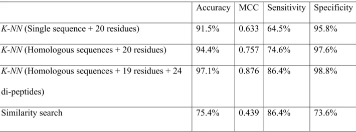
We have developed a weighted Euclidian distance as the distance measurement in our K-NN algorithm. Five-fold cross-validations were used to evaluate performance. For each protein, only the protein itself was used to calculate residue composition. Twenty amino acids were used to calculate the weighted Euclidian distances. As can been see from Table 1 (row 2), the proposed method can distinguish TMB proteins and non-TMB proteins with a 91.5% overall accuracy, with 0.633 MCC. 64.5% (sensitivity) of the TMB proteins, and 95.8% (specificity) of the non-TMB proteins correctly identified.

2.3.2 Including Homologous Sequence Information Improves the Performance

For each of query and training proteins, the BLAST program [26] was used to search for homologous sequences in the NCBI nonredundant database using threshold E=0.0001. At most, 50 best hits plus the protein itself were used to calculate residue

composition. Compositions of all 20 amino acids were used to calculate the weighted Euclidian distances. As can be seen from Table 1 (row 3), the prediction performance can be improved remarkably by including homologous sequence information. The prediction performance was increased to 94.4% overall accuracy, with 0.757 MCC, 74.6%

sensitivity and 97.6% specificity.

2.3.3 Further Improvement of the Prediction Performance by Feature Selection

We tried to include both residue compositions and di-peptide compositions to calculate the WED. However, not all 20+400 features are useful for prediction. After the greedy feature selection process, we obtained a much smaller feature subset, which included 19 residues {A, C, D, E, F, G, H, I, K, L, M, P, Q, R, S, T, V, W, Y} and 24 di-peptides {AI, CC, DP, II, IT, KA, LF, LG, LI, LK, LT, MV, NE, NH, QY, RK, SP, SY, VR, WE, WH, WN, YK, YR }. Using selected features, the prediction performance was further improved to 97.1% accuracy, 0.876 MCC, 86.4% sensitivity and 98.8%

specificity, which can be seen in Table 1 (row 4).

2.3.4 Comparison with Predictions Solely Based on Similarity Search

Similarity searches have been widely used to infer protein functions. If two proteins are highly similar in a sequence, then they might share similar functions, structures or evolutionary origin. For each test protein, we conducted a homologous search on the training set using the BLAST program [26]. The test protein was then predicted to be the protein type (i.e., TMB or non-TMB) of the most homologous protein. Using the same dataset partition and five-fold cross-valuation, the similarity search only

Table 1. Comparison of the Proposed K-NN Method with A Similarity Search.

Accuracy MCC Sensitivity Specificity

K-NN (Single sequence + 20 residues) 91.5% 0.633 64.5% 95.8%

K-NN (Homologous sequences + 20 residues) 94.4% 0.757 74.6% 97.6%

K-NN (Homologous sequences + 19 residues + 24 di-peptides)

97.1% 0.876 86.4% 98.8%

Similarity search 75.4% 0.439 86.4% 73.6%

achieved 75.4% accuracy with 0.439 MCC, 86.4% sensitivity and 73.6% specificity, which was much lower than the proposed K-NN method.

2.3.5 Comparison with Other Prediction Methods

We also compared our method with other state-of-the-art prediction methods, such as TMH-Hunt, BOMP, PRED-TMBB and PROFtmb. All these methods provide web servers, which makes it easy to compare them with our method. Since the number of positive and negative samples is not balanced, MCC was used as the primary

measurement of the prediction performance. Other measurements, such as accuracy, sensitivity and specificity, are also reported.

The datasets used in this study, i.e., both TMB and non-TMB proteins, were submitted to the servers of TMB-Hunt, BOMP, PRED-TMBB and PROFtmb. Table 2 shows the prediction results of all five methods.

Table 2 (row 2) shows the prediction performance of the proposed K-NN method. Homologous sequence information was included to calculate the composition of selected residues and di-peptides. A weighted Euclidian distance is used as distance measurement.

Table 2 (row 3) shows the prediction performance of BOMP [52]. A Blast search option was chosen to ensure highest performance, as mentioned in Section 2.1.3.2.

Table 2 (row 4) gives the prediction results of TMB-Hunt [59, 60]. Evolutionary information was used, which ensures the best performance of the method, as mentioned in Section 2.1.3.1.

Table 2 (row 5) gives the prediction performance of PRED-TMBB [53, 76] using posterior decoding. Three decoding methods are provided on the web server, while the posterior decoding was reported to achieve the best performance.

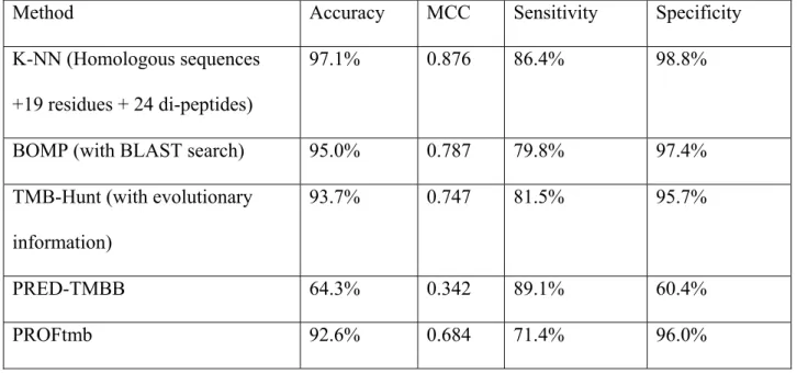
Table 2. Comparison of Different Methods.

Method Accuracy MCC Sensitivity Specificity

K-NN (Homologous sequences +19 residues + 24 di-peptides)

97.1% 0.876 86.4% 98.8%

BOMP (with BLAST search) 95.0% 0.787 79.8% 97.4%

TMB-Hunt (with evolutionary information)

93.7% 0.747 81.5% 95.7%

PRED-TMBB 64.3% 0.342 89.1% 60.4%

10 ≥ Z Z ≥6 ≥ Z 6 ≥ Z

Table 2 (row 6) shows the prediction performance of PROFtmb [20]. The server provides two options: and . We tried both values. PROFtmb achieved better performance with as the threshold. The results reported here were achieved with

.

6

As can be seen from Table 2, the proposed K-NN algorithm outperformed all other methods in both MCC and accuracy. It is worthwhile to point out that the datasets used in the current study are likely to have a big overlap with the datasets that were used to train BOMP, TMB-Hunt, PRED-TMBB, and PROFtmb servers. Thus, when we evaluated these methods by submitting our datasets to their web servers, the performance of these methods might have been overestimated. In contrast, our K-NN method was evaluated using a five-fold cross-validation such that any protein in the training set and any protein in the test set shared less than 25% identity. Remarkably, our method still outperformed the others under this condition.

Another virtue of the proposed K-NN method is its speed. No parameters need to be tuned. The training and prediction processes are simple and efficient. The calculation of residue and di-peptide composition is fast and straightforward. Thus, our method can be applied to scan the whole dataset of gram-negative proteomes for possible TMB proteins. Among the five methods compared, PRED-TMBB and PROFtmb achieved relatively lower performances. However, the major purpose of PRED-TMBB and PROFtmb is to predict the topologies of TMB proteins. The relatively low prediction performances of these methods in the classification of TMB protein can be explained by the following facts: 1) the training datasets only contain positive examples, and there