41
Soret and Dufour Effects on Mixed Convective Heat and Mass
Transfer Flow in a Rectangular Duct with Heat Generating
Sources
C. Sulochana H. Tayappa
Department of Mathematics, Gulbarga University, Gulbarga-585106, Karnataka, India Abstract
In this paper we investigated the combined influence of dissipation, heat sources, Soret and Dufour effects on the convective heat and mass transfer flow of a viscous fluid through porous medium in a rectangular cavity using Darcy model. Making use of the incompressibility the governing non-linear coupled equations for the momentum, energy and diffusion are derived in terms of the non-dimensional stream function, temperature and concentration. The Galerkin finite element analysis with linear triangular elements is used to obtain the Global stiffness matrices for the values of stream function, temperature and concentration. These coupled matrices are solved using iterative procedure and expressions for the stream function, temperature and concentration are obtained as linear combinations of the shape functions. The behaviour of temperature, concentration, Nusselt number and Sherwood number are discussed computationally for different values of the non-dimensional governing parameters.
Keywords: Soret and Dufour effects, heat sources, rectangular duct, finite element analysis.
1. Introduction
Natural convection is of great importance in many industrial applications. Convection plays a dominant role in crystal growth in which it affects the fluid-phase composition and temperature at the phase interface that results in a single crystal since poor crystal quality is due to turbulence. It is the foundation in modern electronics industry to produce pure and perfect crystals to make transistors, lasers rods, microwave devices, infrared detectors, memory devices, and integrated circuits. Natural convection adversely affects local growth conditions and enhances the overall transport rate. The combination of temperature and concentration gradients in the fluid will lead to buoyancy-driven flows. This has an importance influence on the solidification process in a binary system. When heat and mass transfer occurs simultaneously, it leads to a complex fluid motion called double-diffusive convection.
Double-diffusion occurs in a wide range of scientific fields such as oceanography, astrophysics, geology, biology and chemical processes. Ostrach (1887) reported complete reviews on the subject. Bejan (1985) reported a fundamental study of scale analysis relative to heat and mass transfer within cavities submitted to horizontal combined and pure temperature and concentration gradients. Kamotani et al. (1985) considered an experimental study of natural convection in shallow enclosures with horizontal temperature and concentration gradients. Other experimental studies dealing with thermo solutal convection in rectangular enclosures were reported by Lee et al. (1990). Hyun et.al., (1990) reported numerical solutions for unsteady double-diffusive convection in a rectangular enclosure with aiding and opposing temperature and concentration gradients that were in good agreement with reported experimental results. Other related numerical studies dealing with double-diffusive natural convection in cavities were considered by Beghein et al. (1992) and Nishimura et al. (1998). Bera et al. (1998) studied umerically the heat and mass transfer in a anisotropic porous enclosure due to constant heating and cooling. Morega et al (1996) studied double-diffusive convection by chebyshev collocation method, Technol. Electrically conducting fluids in the presence of a magnetic field have been used extensively in many applications such as crystal growth. Oreper and Szekely (1983) have found that the presence of a magnetic field can suppress natural convection currents and that the factors in determining the quality of the crystal. Alchaar et al. (1995) have considered natural convection heat transfer in a rectangular enclosure with a transverse magnetic field. Rudraiah et al. (1995) and Al-Najem et al. (1998) have studied the effects of a magnetic field on free convection in a rectangular enclosure. Researchers Sandeep and Sugunamma (2013), Mohankrishna et al. (2014), Sugunamma and Sandeep (2011), Jayachandra Babu et al. (2015) considered dissipative and radiating fluids and analyzed the flow and heat transfer behaviour through different channels.
Natural convection heat transfer induced by internal heat generation has recently received considerable attention because of numerous applications in geophysics and energy-related engineering problems. Such applications include heat removal from nuclear fuel debris, underground disposal of radioactive waste materials, storage of foodstuff, and exothermic chemical reactions in packed-bed reactor. Kakac et al. (1985) gave fundamentals and applications of natural convection. Strach (1980) analyzed natural convection with combined driving forces. Churbanov et al. (1994) studied numerically unsteady natural convection of a heat generating fluid in a vertical rectangular enclosure with isothermal or adiabatic rigid walls. Their results were obtained
42
using a finite-difference scheme in the two-dimensional stream function-velocity formulation. Steady-state as well as oscillating solutions were obtained and compared with other numerical and experimental published data. Other related works dealing with temperature-dependent heat generation effects can be found in the papers by Vajravelu and Nayfeh (1992) and Chamkha (1999). Sandeep et al. (2012), Sulochana and Sandeep (2015) discussed the heat transfer behaviour of some base and nanofluids in presence of radiation and chemical reaction. Literature suggests that the effect of viscous dissipation on heat transfer as been studied for different geometries. Thermal radiation plays a significant role in the overall surface heat transfer where convective heat transfer is small. Badruddin et al. (2006) have investigated the radiation and viscous dissipation on convective heat transfer in porous cavity. Nishimura et al. (1996) studied the oscillatory double-diffusive convection in a rectangular enclosure with combined horizontal temperature and concentration gradients. Santhi (2011) has investigated double diffusive flow in a rectangular cavity using Darcy model. She has analysed the effect of dissipation radiation on the double diffusive flow of a viscous fluid in the rectangular cavity. Chamka et al. (2002) have investigated the hydromagnetic double-diffusive convection in a rectangular enclosure with opposing temperature and concentration gradients. Sandeep and Sulochana (2015) presented dual solutions for radiative MHD nanofluid flow over an exponentially stretching sheet with heat generation/absorption. Sandeep et al. (2013) studied the radiation effect on the nanofluid flow over a vertical channel. Raju et al. (2015) discussed unsteady boundary layer flow of thermophoretic MHD nanofluid past a stretching sheet with space and time dependent internal heat source/sink. Radiation and soret effects of MHD nanofluid flow over a moving vertical plate in porous medium studied by Raju et al. (2015).
In this paper an attempt has been made to discuss the combined influence of dissipation, heat sources, Soret and Dufour effects on the convective heat and mass transfer flow of a viscous fluid through a porous medium in a rectangular cavity using Darcy model. Making use of the incompressibility the governing non-linear coupled equations for the momentum, energy and diffusion are derived in terms of the non-dimensional stream function, temperature and concentration. The Galerkin finite element analysis with linear triangular elements is used to obtain the Global stiffness matrices for the values of stream function, temperature and concentration. These coupled matrices are solved using iterative procedure and expressions for the stream function, temperature and concentration are obtained as a linear combinations of the shape functions. The behaviour of temperature, concentration, Nusselt number and Sherwood number are discussed. 2. Mathematical Formulation
We consider the mixed convective heat and mass transfer flow of a viscous incompressible fluid in a saturated porous medium confined in the rectangular duct (Fig. 1) whose base length is a and height b. The heat flux on the base and top walls is maintained constant. The Cartesian coordinate system O (x,y) is chosen with origin on the central axis of the duct and its base parallel to x-axis. We assume that the convective fluid and the porous medium are everywhere in local thermodynamic equilibrium. There is no phase change of the fluid in the medium. The properties of the fluid and of the porous medium are homogeneous and isotropic. The porous medium is assumed to be closely packed so that Darcy’s momentum law is adequate in the porous medium. The Boussinesq approximation is applicable. Under these assumption the governing equations are given by
0
=
′
∂
′
∂
+
′
∂
′
∂
y
v
x
u
(1)
′
∂
′
∂
−
=
′
x
p
µ
k
u
(2)
′
+
′
∂
′
∂
−
=
′
ρ
g
y
p
µ
k
v
(3)
′
∂
∂
+
′
∂
∂
+
+
+
+
−
+
′
∂
′
∂
+
′
∂
′
∂
=
′
∂
′
∂
′
+
′
∂
′
∂
′
2 2 2 2 12 2 2 0 2 2 2 2 1(
)
(
)
y
C
x
C
k
v
u
K
T
T
Q
y
T
x
T
K
y
T
v
x
T
u
c
pµ
ρ
σ (4)
′
∂
∂
+
′
∂
∂
+
′
∂
∂
+
′
∂
∂
=
′
∂
∂
′
+
′
∂
∂
′
2 2 2 2 11 2 2 2 2 1y
T
x
T
k
y
C
x
C
D
y
C
v
x
C
u
c
p σρ
(5)43
{
1
(
0)
(
0)
}
0
−
T
′
−
T
−
C
′
−
C
=
′
•β
β
ρ
ρ
(6)2
,
2
0 0 c h c h
C
C
C
T
T
T
=
+
=
+
where u′ and v′ are Darcy velocities along θ(x, y) direction. T′, C,p′ and g′ are the temperature, Concentration,pressure and acceleration due to gravity, Tc ,Cc and Th ,Ch are the temperature and Concentration
on the cold and warm side walls respectively. ρ′, µ, ν, and β are the density, coefficients of viscosity, kinematic viscosity and thermal expansion of he fluid, k is the permeability of the porous medium, K1 is the thermal
conductivity, Cp is the specific heat at constant pressure , Q is the strength of the heat source,k11 and k12 are the
cross diffusivities , β* is the volume coefficient of expansion with mass fraction concentration. The boundary conditions are
u′ = v′ = 0 on the boundary of the duct T′ = Tc ,C=Cc on the side wall to the left
T′ = Th ,C=Ch on the side wall to the right (7)
0 = ∂ ′ ∂ y T ,
=
0
∂
∂
y
C
on the top ( y = 0) and bottom
0
=
=
v
u
walls(y = 0)which are insulated. We now introduce the following non-dimensional variables x′ = ax; ; y′ = by ; c = b/au′ = (ν/a) u ; v′ = (ν/a)v ; p′ = (ν2ρ/a2)p
T′ = T0 + θ (Th – Tc) C′ = C0 + φ (Th – Tc) (8)
The governing equations in the non-dimensional form are
x
p
a
K
u
∂
∂
−
=
2 (9) 2 2 2 2)
(
)
(
v
C
C
kag
v
T
T
kag
v
kag
y
p
a
k
v
−
+
β
h−
cθ
+
β
h−
cφ
∂
∂
−
=
• (10)(
)
∂
∂
+
∂
∂
+
+
+
−
∂
∂
+
∂
∂
=
∂
∂
+
∂
∂
2 2 2 2 2 2 2 2 2 2Pr
y
x
Du
v
u
E
y
x
y
v
x
u
θ
θ
θ
θ
αθ
Cφ
φ
(11) 2 2 2 2 2 2 2 2ScSo
Sc u
v
x
y
x
y
N
x
y
ϕ
ϕ
ϕ
ϕ
θ
θ
∂
∂
∂
∂
∂
∂
+
=
+
+
+
∂
∂
∂
∂
∂
∂
(12)In view of the equation of continuity we introduce the stream function ψ as
x
v
y
u
∂
∂
−
=
∂
∂
=
ψ
;
ψ
(13)Eliminating p from the equation (9) and (10) and making use of (11) the equations in terms of ψ and θ are
)
(
4x
N
x
Ra
∂
∂
+
∂
∂
−
=
∇
ψ
θ
φ
(14) 2 2 2 2 2 2 2 2 2 2Pr
E
CDu
y
x
x
y
x
y
y
x
x
y
ψ
θ
ψ
θ
θ
θ
ψ
ψ
ϕ
ϕ
αθ
∂
∂
∂
∂
∂
∂
∂
∂
∂
∂
−
=
+
−
+
+
+
+
∂
∂
∂
∂
∂
∂
∂
∂
∂
∂
(15)
∂
∂
+
∂
∂
+
∂
∂
+
∂
∂
=
∂
∂
∂
∂
−
∂
∂
∂
∂
2 2 2 2 2 2 2 2y
x
N
ScSo
y
x
y
x
x
y
Sc
ψ
φ
ψ
φ
φ
φ
θ
θ
(16) where 2 3)
(
v
a
T
T
g
G
=
β
h−
c44 α = Qaz/K1(Heat source parameter),
(
)
2ν
β
g
T
T
Ka
Ra
=
g−
c (Rayleigh Number),D
Sc
=
ν
(Schmidt Number),νβ
β
•=
k
11So
(Soret parameter),)
(
)
(
c h c hT
T
C
C
N
−
−
=
∗β
β
(Buoyancy ratio), 4 1a
Ec
KK T
µ
=
∆
(Eckert number),T
C
C
k
Du
p∆
∆
=
ρ
12 (Dufour parameter), The4 boundary conditions are1
&
0
0
,
0
=
=
∂
∂
=
∂
∂
x
on
y
x
ψ
ψ
(17)1,
1
on
x
0
θ
=
ϕ
=
=
0 ,
0
on
x
1
θ
=
ϕ
=
=
(18)3. Finite Element Analysis and Solution of the Problem
The region is divided into a finite number of three node triangular elements, in each of which the element equation is derived using Galerkin weighted residual method. In each element fi the approximate solution for an
unknown f in the variational formulation is expressed as a linear combination of shape function.
( )
N
kik
=
1
,
2
,
3
,
which are linear polynomials in x and y. This approximate solution of the unknown f coincides with actual values at each node of the element. The variational formulation results in a 3 x 3 matrix equation (stiffness matrix) for the unknown local nodal values of the given element. These stiffness matrices are assembled in terms of global nodal values using inter element continuity and boundary conditions resulting in global matrix equation.In each case there are r distinct global nodes in the finite element domain and fp (p = 1,2,……r) is the
global nodal values of any unknown f defined over the domain then
∑
∑
= =
Φ
=
r p p if
f
1 i p 8 1,
where the first summation denotes summation over s elements and the second one represents summation over the independent global nodes and
,
i N i
p
=
N
Φ
if p is one of the local nodes say k of the element ei= 0, otherwise.
fp’ s are determined from the global matrix equation. Based on these lines we now make a finite element
analysis of the given problem governed by (14)-(16) subjected to the conditions (17) – (18). Let ψi
, θi
and φi
be the approximate values of ψ ,θ and φ in an element θi. i i i i i i i
N
N
N
1ψ
1 2ψ
23
ψ
3ψ
=
+
+
i i i i i i iN
N
N
1θ
1 2θ
23
θ
3θ
=
+
+
(19) i i i i i i iN
N
N
1φ
1 2φ
23
φ
3φ
=
+
+
Substituting the approximate value ψi
, θi
and φi
for ψ ,θ and φrespectively in (13), the error
∂
∂
+
∂
∂
+
∂
∂
+
∂
∂
+
+
−
∂
∂
∂
∂
−
∂
∂
∂
∂
−
∂
∂
+
∂
∂
=
2 2 2 2 2 2 2 2 2 2 1y
x
Du
x
y
E
y
x
x
y
P
y
x
E
i i C i i i i i i iφ
φ
ψ
ψ
αθ
θ
ψ
θ
ψ
θ
θ
(20))
(
2 2 2 2 2 2 2 2 2
y
x
N
ScSo
y
x
x
y
Sc
y
x
E
i i i i i i i i i∂
∂
+
∂
∂
+
∂
∂
∂
∂
−
∂
∂
∂
∂
−
∂
∂
+
∂
∂
=
φ
φ
ψ
φ
ψ
φ
φ
φ
(21)45
Under Galerkin method this error is made orthogonal over the domain of ei to the respective shape functions
(weight functions) where
0
1
Ω
=
∫
ei i k id
N
E
,∫
Ω
=
ei i k id
N
E
20
0
3
4
1
(
2 2 2 2 2 2 1=
Ω
∂
∂
+
∂
∂
+
∂
∂
+
∂
∂
+
−
∂
∂
∂
∂
−
∂
∂
∂
∂
−
∂
∂
+
∂
∂
+
∫
=d
y
x
Du
x
y
E
y
x
x
y
P
y
x
N
N
i z i z C ei i i i i i z i z i kφ
φ
ψ
ψ
αθ
θ
ψ
θ
ψ
θ
θ
(22)0
(
2 2 2 2=
Ω
∂
∂
+
∂
∂
+
∂
∂
∂
∂
−
∂
∂
∂
∂
−
∂
∂
+
∂
∂
∫
=d
y
x
N
ScSo
y
x
x
y
Sc
y
x
N
i z i z ei i i i i i z i z i kθ
θ
φ
ψ
φ
ψ
φ
φ
(23)Using Green’s theorem we reduce the surface integral (22) & (23) without affecting ψ terms and obtain
∫
Ω
∂
∂
∂
∂
+
∂
∂
∂
∂
+
∂
∂
+
∂
∂
+
−
∂
∂
∂
∂
−
∂
∂
∂
∂
−
∂
∂
∂
∂
+
∂
∂
∂
∂
ei ki i ki i C i i i i k i i i k i i k i kd
y
y
N
x
x
N
Du
x
y
E
y
x
x
y
N
p
y
y
N
x
x
N
N
)
(
)
(
2 2
φ
φ
ψ
ψ
αθ
θ
ψ
θ
ψ
θ
θ
=∫
ΓΓ
∂
∂
+
∂
∂
i i y i x i i kn
d
y
n
x
N
θ
θ
(24)∫
Ω
∂
∂
∂
∂
+
∂
∂
∂
∂
+
∂
∂
∂
∂
−
∂
∂
∂
∂
−
∂
∂
∂
∂
+
∂
∂
∂
∂
eiei i i k i i k i i i i k i i i k i i k i kd
y
y
N
x
x
N
N
ScSo
y
x
x
y
N
Sc
y
y
N
x
x
N
N
φ
φ
ψ
φ
ψ
φ
(
2θ
θ
)
=∫
ΓΓ
∂
∂
+
∂
∂
+
∂
∂
+
∂
∂
i i y i i x i i i kn
d
y
N
ScSo
y
n
x
N
ScSo
x
N
θ
φ
)
(
θ
φ
(25)where ΓI is the boundary of ei.
Substituting L.H.S. of (19) for ψi , θi and φi in (24) & (25) we get
∫
∑
∑∫
Ω
∂
∂
∂
∂
−
∂
∂
∂
∂
−
∂
∂
∂
∂
+
∂
∂
∂
∂
ei i L i m i L i m i m ei i k i L i L i kd
y
N
x
N
x
N
y
N
P
y
N
y
N
x
N
x
N
1 1
ψ
46
Ω
∂
∂
∂
∂
+
∂
∂
∂
∂
+
∂
∂
+
∂
∂
+
Ω
−
∑ ∫
∫
∑ ∫
Ωd
y
y
N
x
x
N
Du
x
y
E
d
N
N
ei i i k i i k C ei i l k i i)
(
2 2φ
φ
ψ
ψ
θ
α
∫
Γ=
Γ
∂
∂
+
∂
∂
=
i i k i y i x i i kn
d
Q
y
n
x
N
θ
θ
(l, m, k = 1,2,3) (26)∫
∑
∑∫
Ω
∂
∂
∂
∂
−
∂
∂
∂
∂
−
∂
∂
∂
∂
+
∂
∂
∂
∂
ei i L i m i L i m i m ei i k i L i L i k id
y
N
x
N
x
N
y
N
Sc
y
N
y
N
x
N
x
N
)
(
1 1ψ
φ
i ei i i k i L i L i k id
y
N
y
N
x
N
x
N
N
ScSo
∑ ∫
Ω
∂
∂
∂
∂
+
∂
∂
∂
∂
+
θ
(
)
C i i i y i i x i i i kn
d
Q
y
N
ScSo
y
n
x
N
ScSo
x
N
Γ
=
∂
∂
+
∂
∂
+
∂
∂
+
∂
∂
=
∫
Γφ
θ
φ
θ
(
)
(l, m, k = 1,2,3) (27) Where i k i k i k i k i kQ
Q
Q
Q
Q
=
1+
2+
3,
’s being the values ofi k
Q
on the sides s = (1,2,3) of the element ei. The sign of ik
Q
’s depends on the direction of the outward normal w.r.t the element. Choosing differentN
ki’s as weightfunctions and following the same procedure we obtain matrix equations for three unknowns (
Q
ip) viz.,)
(
)
)(
(
ki i p i pQ
a
θ
=
(28)where
(
a
ipk)
is a 3 x 3 matrix,(
θ
pi),
(
Q
ki)
are column matrices.Repeating the above process with each of s elements, we obtain sets of such matrix equations. Introducing the global coordinates and global values for
θ
piand making use of inter element continuity and boundary conditions relevant to the problem the above stiffness matrices are assembled to obtain a global matrix equation. This global matrix is r x r square matrix if there are r distinct global nodes in the domain of flow considered.Similarly substituting ψi
,θi
and φi
in (12) and defining the error
)
x
x
(
Ra
4 3∂
∂
+
∂
∂
+
∇
=
ψ
θ
N
φ
E
i (29)and following the Galerkin method we obtain
0
3Ω
=
∫
Ωd
E
iψ
ij (30)Using Green’s theorem (26) reduces to
∫
Ω
Ω
∂
∂
+
∂
∂
+
∂
∂
∂
∂
+
∂
∂
∂
∂
d
x
N
x
N
y
y
N
x
x
N
ki i ki i i ki i ki(
Ra
ψ
ψ
θ
φ
∫
∫
Γ
Γ
+
ΓΓ
∂
∂
+
∂
∂
=
i i x i k i y i x i i kn
d
N
n
d
y
n
x
N
ψ
ψ
θ
(31)In obtaining (31) the Green’s theorem is applied w.r.t derivatives of ψ without affecting θ terms. Using (19) and (20) in (31) we have
Ω
∂
∂
+
Ω
∂
∂
+
Ω
∂
∂
∂
∂
+
∂
∂
∂
∂
∑
∫
∫
∫
∑
Ω Ω Ω L i L i i L i L i i L i i k i m i m i k i m md
x
N
N
d
x
N
d
y
N
y
N
x
N
x
N
i k i kN
N
(
Ra
θ
φ
ψ
i k i i i k i y i x i i kn
d
N
d
y
n
x
N
Γ
+
Ω
=
Γ
∂
∂
+
∂
∂
=
∫
∫
Γ Γθ
ψ
ψ
(32)
47
In the problem under consideration, for computational purpose, we choose uniform mesh of 10 triangular element (Fig. ii). The domain has vertices whose global coordinates are (0,0), (1,0) and (1,c) in the non-dimensional form. Let e1, e2…..e10 be the ten elements and let θ1, θ2, …..θ10 be the global values of θ and ψ1,
ψ2,……ψ10 be the global values of ψ at the ten global nodes of the domain (Fig. ii).
4.Results and Discussion
In this analysis we investigate the combined influence of dissipation, heat sources, Soret and Dufour effects on convective heat and mass transfer flow through a porous medium in a rectangular duct. The non-linear coupled equations governing the flow of heat and mass transfer have been solved by using Galerkin Finite Element technique with 3-noded triangular elements. We take the Prandtl number Pr = 0.71 in the analysis. The temperature and concentration have been discussed for different variations of Ra, N, α, Sc, So and Ec at different horizontal and vertical levels. The temperature distribution (
θ
) is shown in figures 1-28 for different parametric values at different horizontal levels y= h/3, y=2h/3 and vertical levels x=1/2, x=2/3. We follow the convention that non-dimensional temperatureθ
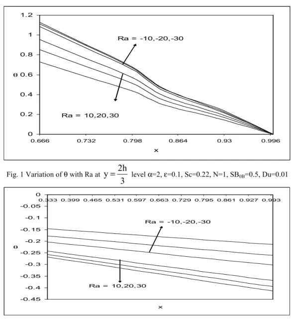
is positive or negative according as the actual temperature T is > or < than Tc, temperature on the cold wall.Figs 1-4 represent the temperature
θ
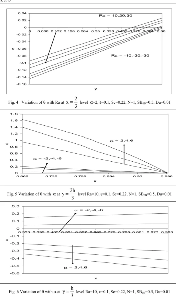
with different values of the Rayleigh number Ra. It is found that the actual temperature enhances at y=h/3 level and vertical levels x=1/3 & x=2/3 and reduces at higher horizontal level y=2h/3 with increase in Ra >0, while increase in |Ra| (<0) reduces the actual temperature at y=h/3, x=1/3 and 2/3 levels and enhances at y=2h/3 level. The effect of heat sources on the temperatureθ
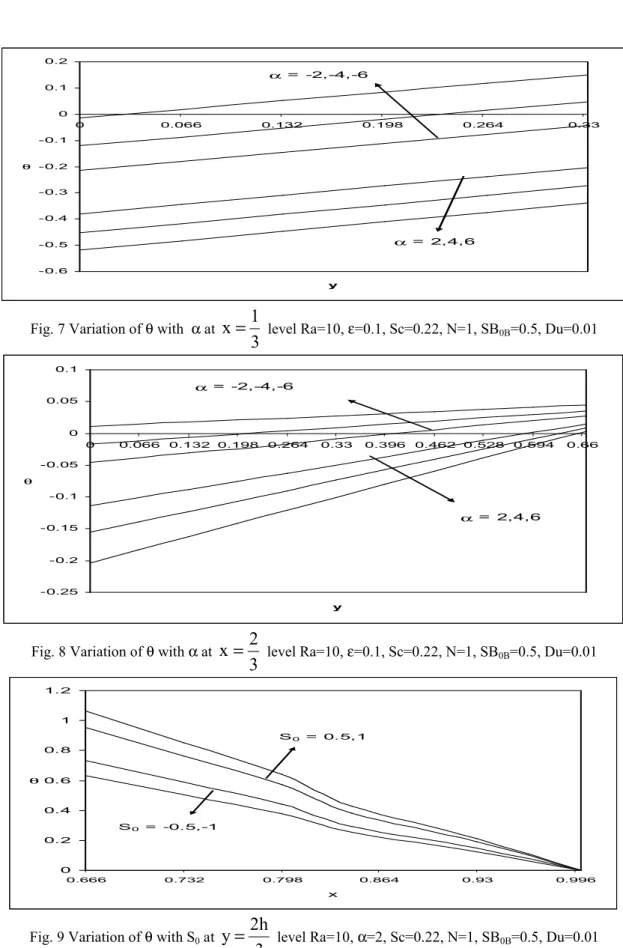
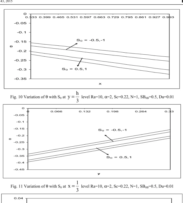
is exhibited in figs 5-8 at different levels. It is found that an increase in the strength of the heat generating sources (α>0) reduces the actual temperature at y=h/3, x=1/3 & x=2/3 levels and enhances at y=2h/3 , while in the case of heat absorbing source the actual temperature enhances at y=h/3, x=1/3 & 2/3 levels and at y=2h/3 level the actual temperature reduces with |α|<4 and for higher |α|>6 we notice an enhancement in the actual temperature in the vertical strip (0.666<0.798) and reduces in the strip (0.846, 0.93).Figs 9-12 represent
θ
with Soret parameter So. It is found that the actual temperature reduces with So >0 at all level, while increase in |So| (<0) enhances the actual temperature at y=h/3, x=1/3 and 2/3 levels and reduces at y=2h/3 level. The influence of Dufour effect (Du) onθ
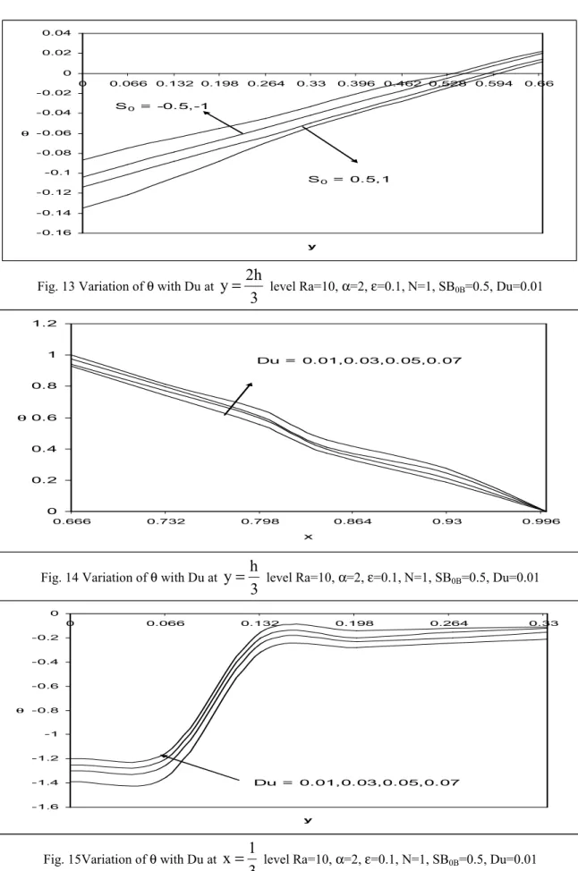
is shown in figs 13-16 at different levels. It is found that the actual temperature enhances at y=h/3, 2h/3 and x=2/3 levels and reduces at x=1/3 level with increase in Du.The rate of heat transfer (Nusselt number) on the side x=1 is shown in the tables 1 and 2 for different parameter variations. It is found that the rate of heat transfer reduces as we move along the vertical direction. The variation of Nu with Rayleigh number Ra and Sc shown that the Nusselt number reduces with increase in Ra and enhances with Sc on all the three quadrants. With reference to heat source parameter αwe find that the Nusselt number enhances with increase in the strength of the heat generating source and reduces with that of heat absorbing source at all levels. With reference to buoyancy ratio N, we find that when the molecular buoyancy force dominates over the thermal buoyancy force, the Nusselt number on the lower and middle quadrants reduces and enhances on the upper most quadrant when the buoyancy forces are in the same direction and for the forces acting in opposite direction the Nusselt number enhances on lower quadrant and reduces on the middle & upper quadrant (table-1). The variation of Nu with Ec shows that higher the dissipative heat larger the Nusselt number on the lower and middle quadrants and reduces on the upper quadrant. With reference to So we find that the Nusselt number enhances with increase in So >0 and reduces with |So|<o on all the three quadrants. Also higher the diffusion thermo effect smaller the Nusselt number on all the three quadrants
48 Fig. 1 Variation of θ with Ra at
3
2h
y
=
level α=2, ε=0.1, Sc=0.22, N=1, SB0B=0.5, Du=0.01Fig. 2 Variation of θ with Ra at
3
h
y
=
level α=2, ε=0.1, Sc=0.22, N=1, SB0B=0.5, Du=0.01Fig. 3 Variation of θ with Ra at
3
1
x
=
level α=2, ε=0.1, Sc=0.22, N=1, SB0B=0.5, Du=0.01 0 0.2 0.4 0.6 0.8 1 1.2 0.666 0.732 0.798 0.864 0.93 0.996 x θ Ra = -10,-20,-30 Ra = 10,20,30 -0.45 -0.4 -0.35 -0.3 -0.25 -0.2 -0.15 -0.1 -0.05 0 0.333 0.399 0.465 0.531 0.597 0.663 0.729 0.795 0.861 0.927 0.993 x θ Ra = -10,-20,-30 Ra = 10,20,30 -0.5 -0.45 -0.4 -0.35 -0.3 -0.25 -0.2 -0.15 -0.1 -0.05 0 0 0.066 0.132 0.198 0.264 0.33 y θ Ra = 10,20,30 Ra = -10,-20,-3049 Fig. 4 Variation of θ with Ra at
3
2
x
=
level α=2, ε=0.1, Sc=0.22, N=1, SB0B=0.5, Du=0.01Fig. 5 Variation of θ with α at
3
2h
y
=
level Ra=10, ε=0.1, Sc=0.22, N=1, SB0B=0.5, Du=0.01Fig. 6 Variation of θ with α at
3
h
y
=
level Ra=10, ε=0.1, Sc=0.22, N=1, SB0B=0.5, Du=0.01-0.16 -0.14 -0.12 -0.1 -0.08 -0.06 -0.04 -0.02 0 0.02 0.04 0 0.066 0.132 0.198 0.264 0.33 0.396 0.462 0.528 0.594 0.66 y θ Ra = 10,20,30 Ra = -10,-20,-30 0 0.2 0.4 0.6 0.8 1 1.2 1.4 1.6 1.8 0.666 0.732 0.798 0.864 0.93 0.996 x θ α = 2,4,6 α = -2,-4,-6 -0.6 -0.5 -0.4 -0.3 -0.2 -0.1 0 0.1 0.2 0.3 0.333 0.399 0.465 0.531 0.597 0.663 0.729 0.795 0.861 0.927 0.993 x θ α = 2,4,6 α = -2,-4,-6
50 Fig. 7 Variation of θ with α at
3
1
x
=
level Ra=10, ε=0.1, Sc=0.22, N=1, SB0B=0.5, Du=0.01Fig. 8 Variation of θ with α at
3
2
x
=
level Ra=10, ε=0.1, Sc=0.22, N=1, SB0B=0.5, Du=0.01Fig. 9 Variation of θ with S0 at
3
2h
y
=
level Ra=10, α=2, Sc=0.22, N=1, SB0B=0.5, Du=0.01 -0.6 -0.5 -0.4 -0.3 -0.2 -0.1 0 0.1 0.2 0 0.066 0.132 0.198 0.264 0.33 y θ α = 2,4,6 α = -2,-4,-6 -0.25 -0.2 -0.15 -0.1 -0.05 0 0.05 0.1 0 0.066 0.132 0.198 0.264 0.33 0.396 0.462 0.528 0.594 0.66 y θ α = 2,4,6 α = -2,-4,-6 0 0.2 0.4 0.6 0.8 1 1.2 0.666 0.732 0.798 0.864 0.93 0.996 x θ S0 = 0.5,1 S0 = -0.5,-151 Fig. 10 Variation of θ with S0 at
3
h
y
=
level Ra=10, α=2, Sc=0.22, N=1, SB0B=0.5, Du=0.01Fig. 11 Variation of θ with S0 at
3
1
x
=
level Ra=10, α=2, Sc=0.22, N=1, SB0B=0.5, Du=0.01Fig. 12 Variation of θ with S0 at
3
2
x
=
level Ra=10, α=2, Sc=0.22, N=1, SB0B=0.5, Du=0.01-0.35 -0.3 -0.25 -0.2 -0.15 -0.1 -0.05 0 0.333 0.399 0.465 0.531 0.597 0.663 0.729 0.795 0.861 0.927 0.993 x θ S0 = 0.5,1 S0 = -0.5,-1 -0.45 -0.4 -0.35 -0.3 -0.25 -0.2 -0.15 -0.1 -0.05 0 0 0.066 0.132 0.198 0.264 0.33 y θ S0 = 0.5,1 S0 = -0.5,-1 -0.14 -0.12 -0.1 -0.08 -0.06 -0.04 -0.02 0 0.02 0.04 0 0.066 0.132 0.198 0.264 0.33 0.396 0.462 0.528 0.594 0.66 y θ ε = 0.1,0.3,0.5
52 Fig. 13 Variation of θ with Du at
3
2h
y
=
level Ra=10, α=2, ε=0.1, N=1, SB0B=0.5, Du=0.01Fig. 14 Variation of θ with Du at
3
h
y
=
level Ra=10, α=2, ε=0.1, N=1, SB0B=0.5, Du=0.01Fig. 15Variation of θ with Du at
3
1
x
=
level Ra=10, α=2, ε=0.1, N=1, SB0B=0.5, Du=0.01-0.16 -0.14 -0.12 -0.1 -0.08 -0.06 -0.04 -0.02 0 0.02 0.04 0 0.066 0.132 0.198 0.264 0.33 0.396 0.462 0.528 0.594 0.66 y θ S0 = 0.5,1 S0 = -0.5,-1 0 0.2 0.4 0.6 0.8 1 1.2 0.666 0.732 0.798 0.864 0.93 0.996 x θ Du = 0.01,0.03,0.05,0.07 -1.6 -1.4 -1.2 -1 -0.8 -0.6 -0.4 -0.2 0 0 0.066 0.132 0.198 0.264 0.33 y θ Du = 0.01,0.03,0.05,0.07
53 Fig. 16 Variation of θ with Du at
3
2
x
=
level Ra=10, α=2, ε=0.1, N=1, SB0B=0.5, Du=0.01I II III IV V VI VII Nu1 3.341757 3.313125 3.466986 3.137157 3.050394 3.340593 3.33255 Nu2 3.1493595 3.1261704 3.2209167 3.02723856 2.97211446 3.1476702 3.1468878 Nu3 2.9569617 2.9392164 2.97484725 2.9173203 2.894694 2.9547474 2.9612259 Ra 10 20 10 10 10 10 10 Sc 1.3 1.3 1.3 1.3 1.3 0.66 1.3 N 1 1 1 1 1 1 2
Table 2 Nusselt Number Nu at x=2/3
I II III IV V VI Nu1 3.342975 3.345429 3.356769 3.311673 3.2965374 3.341676 Nu2 3.1498278 3.1507659 3.1612887 3.1257351 3.1139961 3.1474062 Nu3 2.9566818 2.9561025 2.9658075 2.9397981 2.932548 2.9531352 Ec 0.01 0.03 0.01 0.01 0.01 0.01 So 0.5 0.5 1 -0.5 -1 0.5 Du 0.05 0.05 0.05 0.05 0.05 0.07 5. Conclusions
This paper presents the numerical solution of combined influence of dissipation, heat sources, Soret and Dufour effects on the convective heat and mass transfer flow of a viscous fluid through porous medium in a rectangular cavity using Darcy model. Making use of the incompressibility the governing non-linear coupled equations for the momentum, energy and diffusion are derived in terms of the non-dimensional stream function, temperature and concentration. The conclusions of the present study are made as follows:
• An increase in Rayleigh number causes to increase in the temperature profiles in vertical level and reduces in horizontal level.
• A raise in the value of heat source parameter enhances the temperature profiles of the flow. • For higher values of the dissipative heat enhances the actual temperature.
• Decrease in molecular diffusivity depreciates actual temperature at both the vertical and horizontal levels.
References
Alchaar S., Vasseur, P., Bilgen, E. (1995). Natural convection heat transfer in a rectangular enclosure with a transverse magnetic field, ASME J. Heat Transfer 117, pp.668-63.
Al-Najem, N.M., Khanafer K.M., El-Refaee M.M. (1998). Numerical study of laminar natural convection in tilted enclosure with transverse magnetic field, Int. J. Numer. Meth. Heat Fluid Flow, 8, pp.651-672. Badruddin, I. A, Zainal, Z.A, Aswatha Narayana, Seetharamu, K.N. (2006). Heat transfer in porous cavity under
the influence of radiation and viscous dissipation, Int. Comm. In Heat & Mass Transfer 33, pp 491-499. Beghein, C., Haghighat, F, Allard F, (1992). Numerical study of double – diffusive natural convection in a
square cavity, Int. J. Heat Mass Transfer, 35, pp.833-846.
Bejan, A. (1985). Mass and heat transfer by natural convection in a vertical cavity. Int. J. Heat Fluid Flow, 6,
- 0.14 - 0.12 -0.1 - 0.08 - 0.06 - 0.04 - 0.02 0 0.02 0.04 0 0.066 0.132 0.198 0.264 0.33 0.396 0.462 0.528 0.594 0.66 y θ Du = 0.01,0.03, 0.05,0. 07
54 149-159.
Bera, P. Eswaran, V., Singh P. (1998). Numerical study of heat and mass transfer in a anisotropic porous enclosure due to constant heating and cooling, Numer. Heat Transfer A 34, pp. 887-905.
Chamkha A.J. (1997). Non-Darcy fully developed mixed convection in a porous medium channel with heat generation absorption and hydromagnetic effects, Numer. Heat Transfer 32, pp.653- 675.
Chamkha, A.J., Hameed Al-Naser (2002). Hydromagnetic double-diffusive convection in a rectangular enclosure with opposing temperature and concentration gradients, Int. J. of Heat and Mass Transfer, 45, pp.2465-2483.
Churbanov, A.G., Vabishchevich P.N., Chudanov. V.V., Strizhov V.F. (1994). A numerical study on natural convection of a heat-generating fluid in rectangular enclosures, Int. J. Heat Mass Transfer, 37, pp.2969-2984.
Hyun, J.M., Lee, J.W. (1990). Double-diffusive convective in a rectangle with cooperating horizontal gradients of temperature and concentration gradients. Int. J. Heat Mass Transfer 33, pp.1605-1617.
Jayachandra Babu, M., Radha Gupta and Sandeep, N. (2015). Effect of radiation and viscous dissipation on stagnation-point flow of a micropolar fluid over a nonlinearly stretching surface with suction/injection, Journal of Basic and Applied Research International, vol. 7(2), pp. 73-82.
Kakac, S., Aung. W., Viskanta. R.(1998). Natural Convection Fundamentals and Applications, Hemisphere, Washington, DC.
Kamotani, Y., Wang. L.W., Ostrach S., Jiang H.D. (1985). Experimental study of natural convection in shallow enclosures with horizontal temperature and concentration gradients. Int. J. Heat Mass Transfer 28, 165-173.
Lee, J.W., Hyun, J.M. (1990). Double-diffusive convection in a rectangle with opposing horizontal and concentration gradients. Int. J. Heat Mass Transfer 33, 1619-1632.
Mohankrishna, P., Sugunamma, V. and Sandeep, N. (2014). Radiation and magneticfield effects on unsteady natural convection flow of a nanofluid past an infinite vertical plate with heat source, Chemical and Process Engineering Research, 25, pp.39-52.
Morega, A.M., Nishimura T. (1996). Double-diffusive convection by Chebyshev collocation method, Technol. Rep. Yamaguchi Univ. 5, pp.259-276.
Nishimura, T., Wakamatsu M., Morega A.M. (1998). Oscillatory Double-diffusive convection in a rectangular enclosure with combined horizontal temperature and concentration gradients, Int. J. Heat Mass Transfer 41, pp.1601-1611.
Nithiarasu, P., Seetharamu K.N., Sundararajan T. (1996). Double-diffusive natural convection in an enclosure filled with fluid-saturated porous medium: a generalized non-Darcy approach, Number. Heat Transfer A 30, pp.413-426.
Strach, S. (1980). Natural convection with combined driving forces. Physico Chem. Hydrodyn. 1, pp.233-247. Oreper, G.M., Szekely J. (1983). The effect of an externally imposed magnetic field on buoyancy driven flow in
a rectangular cavity, J. Cryst. Growth 64, pp.505-515.
Ostrach, S., Jiang H.D., Kamotani Y. (1987). Thermo-solutal convection in shallow enclosures. ASME-JSME Thermal Engineering Joint Conference, Hawali.
Raju, C. S. K. , Jayachandra Babu, M. , Sandeep, N., Sugunamma, V., Reddy J.V.R. (2015) Radiation and soret effects of MHD nanofluid flow over a moving vertical plate in porous medium. Chemical and Process Engineering Researc, 30, 9-23.
Raju, C.S.K., Sandeep, N., Sulochana, C., Sugunamma, V., Jayachandra Babu, M. (2015).
Radiation, Inclined Magnetic field and Cross-Diffusion effects on flow over a stretching surface. Journal of Nigerian Mathematical Society (In Press)
Rudraiah, N., Barron R.M., Venkatachalappa M., Subbaraya, C.K. (1995). Effect of a magnetic field on free convection in a rectangular enclosure, Int. J. Eng. Sci. 33, pp.1075-1084.
Sandeep, N., Reddy, A.V.B, Sugunamma, V. (2012). Effect of radiation and chemical reaction on transient MHD free convective flow over a vertical plate through porous media. Chemical and process engineering research. 2, 1-9.
Sandeep, N. and Sugunamma, V. (2013). Effect of inclined magneticfield on unsteady free convection flow of a dusty viscous fluid between two infinite flat plates filled by porous medium. Int.J.App.Math.Modeling, 1, 16-33.
Sugunamma, V. and Sandeep, N. (2011). Unsteady hydrmagnetic free convection flow of a dissipative and radiating fluid past a vertical plate through porous media with constant heat flux. International journal of mathematics and computer applications research, 1, 37-50.
Sandeep, N., Sugunamma, V., and Mohankrishna, P. (2013). Effects of radiation on an unsteady natural convective flow of a EG-Nimonic 80a nanofluid past an infinite vertical plate, Advances in Physics Theories and Applications, 23, pp.36-43.
55
Sandeep, N. and Sulochana, C. (2015). Dual solutions of radiative MHD nanofluid flow over an exponentially stretching sheet with heat generation/absorption, App. Nano. Science 5, (In Press) DOI 10.1007/s13204-015-0420-z, 2015.
Sulochana, C., and Sandeep, N. (2015). Stagnation-point flow and heat transfer behavior of Cu-water nanofluid towards horizontal and exponentially stretching/shrinking cylinders, Applied Nanoscience, 5, (In Press). Vajravelu K., Nayfeh J. (1992). Hydromagnetic convection at a cone and a wedge, Int. Commun. Heat Mass
More information about the firm can be found on the homepage:
http://www.iiste.org
CALL FOR JOURNAL PAPERS
There are more than 30 peer-reviewed academic journals hosted under the hosting platform.
Prospective authors of journals can find the submission instruction on the following
page:
http://www.iiste.org/journals/
All the journals articles are available online to the
readers all over the world without financial, legal, or technical barriers other than those
inseparable from gaining access to the internet itself. Paper version of the journals is also
available upon request of readers and authors.
MORE RESOURCES
Book publication information: http://www.iiste.org/book/
Academic conference: http://www.iiste.org/conference/upcoming-conferences-call-for-paper/
IISTE Knowledge Sharing Partners
EBSCO, Index Copernicus, Ulrich's Periodicals Directory, JournalTOCS, PKP Open
Archives Harvester, Bielefeld Academic Search Engine, Elektronische Zeitschriftenbibliothek
EZB, Open J-Gate, OCLC WorldCat, Universe Digtial Library , NewJour, Google Scholar