2017
Engineering analytics through explainable deep
learning
Sambuddha Ghosal
Iowa State UniversityFollow this and additional works at:
https://lib.dr.iastate.edu/etd
Part of the
Agriculture Commons,
Computer Sciences Commons,
Mechanical Engineering
Commons, and the
Plant Sciences Commons
This Thesis is brought to you for free and open access by the Iowa State University Capstones, Theses and Dissertations at Iowa State University Digital Repository. It has been accepted for inclusion in Graduate Theses and Dissertations by an authorized administrator of Iowa State University Digital Repository. For more information, please [email protected].
Recommended Citation
Ghosal, Sambuddha, "Engineering analytics through explainable deep learning" (2017).Graduate Theses and Dissertations. 16277.
by
Sambuddha Ghosal
A thesissubmittedtothegraduatefaculty
inpartialfulfillmentoftherequirementsforthedegreeof
Major: MechanicalEngineering
Program ofStudy Committee:
Soumik Sarkar,MajorProfessor
BaskarGanapathysubramanian
ArtiSingh
The studentauthor,whosepresentationof thescholarshiphereinwasapprovedbytheprogramof
studycommittee,is solelyresponsible forthecontentof thisthesis. TheGraduate Collegewill
ensurethisthesisis globallyaccessibleand willnotpermit alterationsafter adegree isconferred.
IowaState University
Ames, Iowa
2017
MASTEROF SCIENCE
DEDICATION
TABLE OF CONTENTS Page LIST OF FIGURES . . . vi ACKNOWLEDGEMENTS . . . xi ABSTRACT . . . xii CHAPTER 1. INTRODUCTION . . . 1 1.1 Motivation . . . 1 1.2 Literature Survey . . . 1
1.2.1 Object Recognition via Handcrafting of Features . . . 2
1.2.2 Object Detection via Handcrafting of Features . . . 2
1.2.3 Neural Networks applied in Object Detection and Feature Learning . . . 3
1.3 Thesis Organization . . . 5
CHAPTER 2. PRELIMINARIES ON DEEP LEARNING AND TRAINING CONSIDER-ATIONS . . . 6
2.1 Restricted Boltzmann Machines (RBMs) . . . 6
2.2 Deep Neural Networks . . . 8
2.3 Deep Convolutional Neural Networks (DCNNs) . . . 9
2.3.1 Overview of the different layers used in DCNNs . . . 12
2.4 Gradient-weighted Class Activation Mapping (Grad-CAM) . . . 14
2.5 Convolutional Autoencoders . . . 16
2.6 Training Considerations . . . 17
2.6.1 Data Preprocessing . . . 17
2.6.4 Activation Functions . . . 19
CHAPTER 3. EXPLAINABLE AND APPLIED 2D DEEP LEARNING: BRINGING CON-SISTENCY TO PLANT STRESS PHENOTYPING . . . 21
3.1 Severity Rating by Human Experts using a Visual Application . . . 23
3.2 Leaf Sample Collection and Data Generation . . . 24
3.2.1 Data Collection . . . 26
3.2.2 Data Preparation and Generation . . . 28
3.3 Deep CNN Model and Explanation Framework . . . 29
3.3.1 Network Parameters . . . 29
3.3.2 Training the DCNN . . . 30
3.4 Results . . . 30
3.4.1 Disease Classification and Identification . . . 30
3.4.2 Symptom Explanation and Severity Quantification . . . 31
3.5 Discussions . . . 37
3.5.1 Transfer Learning Capability . . . 38
CHAPTER 4. EXPLAINABLE AND APPLIED 3D DEEP LEARNING: EARLY DETEC-TION OF COMBUSDETEC-TION INSTABILITIES FROM HIGH-SPEED VIDEO . . . 41
4.1 Problem Formulation and Experimental Setup . . . 43
4.1.1 Problem Statement . . . 43
4.1.2 Experimental Setup and Description . . . 45
4.2 Dataset Generation . . . 45
4.3 Network Architecture . . . 46
4.4 Results . . . 48
4.4.1 Results from the 3D CNN model . . . 48
4.4.2 Comparing the 3D-CNN based results with a 2D-based method, 2D CAE . . 49
4.4.3 Explaining the results with 3D CAE . . . 50
REFERENCES . . . 54
LIST OF FIGURES
Page
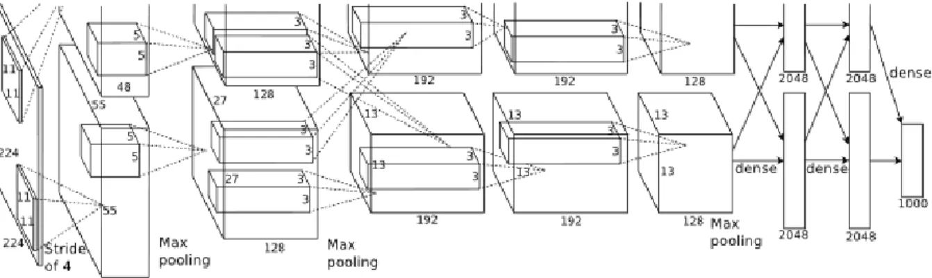
Figure 1.1 Reproduced from (39): The CNN architecture crafted for the 1000 category
ImageNet classification, explicitly showing the delineation of responsibilities between two GPUs. One GPU runs the layer-parts at the top of the figure while the other runs the layer-parts at the bottom. The GPUs communicate only at certain layers. The networks input is 150,528-dimensional, and the number of neurons in the networks remaining layers is given by 253, 440
-186, 624 - 64, 896 - 64, 896 - 43, 264 - 4096 - 4096 - 1000. . . 4
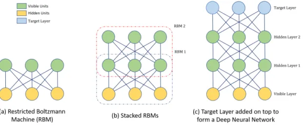
Figure 2.1 Differentiation between Boltzmann machines and Restricted Boltzmann ma-chines (RBMs). In RBMs, there are no interconnections between the nodes in the same layer i.e., there are novisible-visible orhidden-hiddenconnections. 7 Figure 2.2 Stacking of RBMs to form a Deep Neural Network . . . 8
2.3 Illustration showing how 2D Convolution works . . . 10
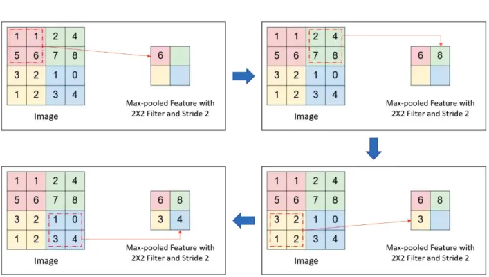
2.4 Illustration showing how 2D Max-Pooling works . . . 11
2.5 Illustration of a typical Convolutional Neural Network architecture . . . 12
2.6 Illustration of the Grad-CAM algorithm . . . 15
2.7 Illustration of a typical Convolutional Auto-Encoder architecture . . . 16
2.8 Data Preprocessing techniques. Illustration Courtesy: Stanford CS231n lec-ture notes . . . 17
2.9 The idea behind performing Batch Normalization. Illustration Courtesy: Stanford CS231n lecture notes . . . 18
2.10 Dropout takes care of over-fitting issues by randomly dropping activation units. Illustration Courtesy: Stanford CS231n lecture notes . . . 19
Figure Figure Figure Figure Figure Figure Figure Figure
3.1 Design of the web app for expert-based foliar disease identification and
sever-ity estimation . . . 24
3.2 Illustration showing the tagging process . . . 25
3.3 Leaf Imaging Platform . . . 26
3.4 Schematic illustration of foliar plant stresses in soybean grouped into two
major categories, biotic (bacterial and fungal) and abiotic (nutrient
de-ficiency and chemical injury) stress. The images were used to develop
the DCNN for the following eight stresses: bacterial blight (Pseudomonas
savastanoi pv. glycinea), bacterial pustule (Xanthomonas axonopodis pv.
glycines), sudden death syndrome (SDS, Fusarium virguliforme), Septoria
brown spot (Septoria glycines), frogeye leaf spot (Cercospora sojina), IDC,
potassium deficiency and herbicide injury. For each stress, information such as symptom descriptors, areas of appearance and most commonly mistaken stresses that exhibit similar symptoms are listed. These particular foliar stresses were chosen because of their large economic impact on agriculture
and confounding symptoms. . . 27
3.5 Illustration of data augmentation scheme . . . 28
3.6 Variation of test accuracy w.r.t. the increasing size of training data . . . 31
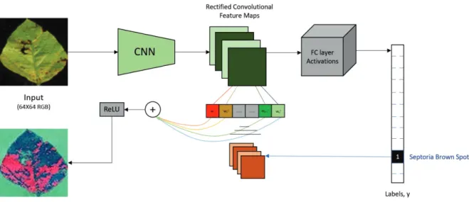
3.7 (a) DCNN architecture used. (b) Prediction Explanation Phase. The
con-cept of gradient-based class activation mapping (Grad-CAM) was applied to automatically visualize image features used by the DCNN model when
making a classification decision. . . 32
Figure Figure Figure Figure Figure Figure Figure
3.8 (a) This confusion matrix shows the stress classification results of the DCNN model for eight different stresses and healthy leaves. The overall classifica-tion accuracy of the model is 94%. The greatest confusion among stresses was found among bacterial blight, bacterial pustule, and Septoria brown spot. A reasonable explanation for these higher failure rates can be at-tributed to the similarities in symptom expression among these stresses.(b) is a scatter plot comparing the severity ratings of the same images between two raters for four stresses (IDC, SDS, potassium deficiency and Septoria
brown spot) that were pooled and solid red line is the 45o line. The results
indicated high inter-rater variability between experienced raters, especially
as the stress severity of leaf images increase. . . 33
3.9 This table presents leaf image examples for each soybean stress identified and classified by the DCNN model. The Grad-CAM framework was applied to highlight regions of interest (symptoms) extracted by the DCNN model. These automatically extracted symptoms were compared against versions of
images with symptoms that were marked manually by expert raters. . . 34
3.10 Rater-based severity versus ML severity scatter plots (pre-calibration: left and post-calibration: right) for class 1: Septoria brown spot. The solid red line is the reference 45-degree slope line and the dashed red line shows the
linear fit applied to the points on the scatter plot in both cases. . . 35
Figure
Figure
3.11 These figures (a, b, c) details the comparison between human and machine learning-based severity ratings for three previously mentioned stresses [(a) Septoria brown spot, (b) IDC, and (c) Sudden Death Syndrome]. The sever-ity comparison using a standard discretized seversever-ity scale (0-15%: resis-tant, 15-30%: moderately resisresis-tant, 30-45%: moderately susceptible, 45-75%: susceptible, and 75-100%: highly susceptible) shows the success of the DCNN-based severity estimation framework to correctly quantify symp-toms for these stresses. Classes such as resistance and highly susceptible tended to have high accuracy across the three stresses, whereas classes such
as moderately susceptible were associated with greater confusion. . . 38
3.12 Examples in which Grad-CAM failed to detect proper disease signatures . . 39
Figure 3.13 This table illustrates the ability of the Grad-CAM framework to accurately
identify the same stress symptoms used in training the DCNN model to non-soybean crops, such as frogeye leaf spots in apple leaves, IDC in cucurbits
and potassium deficiency in oilseed rape. . . 40
Figure 4.1 (a):Schematic of the experimental setup. 1 - settling chamber, 2 - inlet duct,
3 - IOAM, 4 - test section, 5 - big extension duct, 6 - small extension ducts,
7 - pressure transducers, Xs - swirler location measured downstream from
settling chamber exit,Xp - transducer port location measured downstream
from settling chamber exit, Xi - fuel injection location measured upstream
from swirler exit, (b):Swirler assembly used in the combustor. . . 44
Figure 4.2 Combustionimagesusedforflamestabilityanalysis,capturedat3000f ps ;
(f rames/second)i.e.3kHzTop: greyscaleimages atRe=7,971and full
premixingforafuelflowrateof0.495g/s,bottom:greyscaleimagesatRe=
15,942andfullpremixing
forafuelflowrateof0.495g/s.(ImageSource:(99)) 46
Figure 4.3 Description of operating conditions along with respective ground truth
(sta-ble or unsta(sta-ble) for hi-speed image data collection. . . 47
Figure
Figure 4.4 Examples of stable and unstable flame frames in a typical temporal evolution
and their respective 3D super-voxels. . . 48
Figure 4.5 3D CNN architecture consisting of example image snapshots, hierarchical
layers and model parameters that were trained to learn the suitable features
from frames in the stable and unstable frames. . . 48
Figure 4.6 3D CNN Results for the 3 considered protocols with example frames from
each of the unstable intermittencies in the insets. . . 49
Figure 4.7 2D CAE Results for the 3 considered protocols. . . 50
Figure 4.8 Illustration of CAE’s ability to segregate regions of stability from
ACKNOWLEDGEMENTS
I would like to take this opportunity to express my thanks to those who helped me with various aspects of conducting research throughout my graduate education and the writing of this thesis.
First and foremost, Dr. Soumik Sarkar for his guidance, patience and support throughout this research and the writing of this thesis. His insights and words of encouragement have often inspired me and renewed my hopes for completing my graduate education.
I would also like to thank my committee members, Dr. Baskar Ganapathysubramanian and Dr. Arti Singh for their valuable efforts and contributions in helping me to bring this work to fruition. I would additionally like to thank Dr. James Michael for his guidance throughout the later stages of preparing my thesis.
ABSTRACT
Pattern recognition has its origins in engineering while machine learning developed from com-puter science. Today, artificial intelligence (AI) is a booming field with many practical applications and active research topics that deals with both pattern recognition and machine learning. We now use softwares and applications to automate routine labor, understand speech (using Natural Lan-guage Processing) or images (extracting hierarchical features and patterns for object detection and pattern recognition), make diagnoses in medicine, even intricate surgical procedures and support basic scientific research.
This thesis deals with exploring the application of a specific branch of AI, or a specific tool, Deep Learning (DL) to real world engineering problems which otherwise had been difficult to solve using existing methods till date. Here we focus on different Deep Learning based methods to deal with two such engineering problems. We also explore the inner workings of such models through an explanation stage for each of the applied DL based strategies that gives us a sense of how such typical black box models work, or as we call it, an explanation stage for the DL model.
This explanation framework is an important step as previously, Deep Learning based models were thought to be frameworks which produce good results (classification, object detection, object recognition to name a few), but with no explanations or immediately visible causes as to why it achieves the results it does. This made Deep Learning based models hard to trust amongst the scientific community. In this thesis, we aim to achieve just that by deploying two such explanation frameworks, one for a 2D image study case and another for a 3D image voxel study case, which will be discussed later in the subsequent chapters.
CHAPTER 1. INTRODUCTION
In this chapter, a short introduction to the concept of Deep Learning is put forth. Section 1.1
discusses the motivation for carrying out this research and a brief literature survey is presented in
section 1.2.
1.1 Motivation
Deep Learning (referred to as ”DL” from here on), in general is a very powerful tool that deals with solving tasks that are easy for people to perform but at the same time hard for people to describe formally i.e., problems that are more intuitive, for instance, recognizing words or faces in in images. This kind of methods allow computers to learn from experience and understand their surroundings in terms of hierarchy of concepts, with each concept defined through its relation to simpler concepts. This hierarchy of concepts enables the computer to learn complicated concepts by building them out of simpler ones.
In recent times, DL models have been shown to outperform other state of the art techniques in handling and analyzing large dimensional data (both spatial and temporal), by learning the hierarchical features to perform various tasks such as, classification and bulk structure detection given a large corpus of 2-dimensional (2D) data or images. As an extension, embedding of 3-dimensional (3D) spatiotemporal data (where the data have spatial features evolving over time) has also been performed using a 3D Convolutional Neural Network (3D CNN) framework.
1.2 Literature Survey
Deep Learning has proved its mettle in various fields of modern science such as medical imaging applications that have achieved dermatologist level classification accuracies for skin cancer (1), in modeling neural responses and population in visual cortical areas of the brain (2) and in
predict-ing sequence specificities of DNA- and RNA-bindpredict-ing proteins (3). Similarly, deep learnpredict-ing based techniques have made transformative demonstration in the context of performing complex cogni-tive tasks such as achieving human level or better accuracy for playing Atari games using Deep Q network (4) and beating a human expert in playing the Chinese game of Go (5).
1.2.1 Object Recognition via Handcrafting of Features
Appearance of an image region has been effectively described by this method, although it has proved to be time-consuming and resource intensive. SIFT (Scale Invariant Feature Transform)(6), HoG (histogram of Gradients)(7), LBP (Local Binary Pattern)(8) are some low-level techniques that follow handcrafting. These essentially describe the low order statistics of the edge distribution where each image region generate fixed size vector to describe properties of the region. SIFT describes the appearance of an image, HoG describes edges and LBP describes textures. Thus, depending on the task at hand, these techniques can be used separately (9)(10)(11) or can be combined (15).
Probabilistic graphical models (12, 13, 14) have also been successful in various image-recognition tasks by building on low level handcrafted features. Probabilistic models can model object shapes, appearance, occlusion and relative scales quite efficiently. One such modeling technique is to learn the parameters of a model to maximize object likelihood in an image with expectation-maximization (EM) algorithm. A ”generic” knowledge learnt by graphical models can even be applied to models of unrelated categories as ”prior” knowledge.
1.2.2 Object Detection via Handcrafting of Features
Object detection can be performed using handcrafted features. Detection systems have been built based on ”part-based” models (10, 15, 16, 17, 18, 19, 20) with patch appearance features like HoG (Histogram of Gradient) (7), SIFT (Scale Invariant Feature Transform) (6), LBP (Local Binary Pattern) (8). These are general object detection models, an significant achievement in
computer vision that requires prediction of object labels and object locations at the same time. Pedestrian detection with HoG features (7) is one such example.
Different object detection results can enhance or inhibit each other within a scene or context. Active research in object recognition has been carried out on this part (21, 22, 23, 24, 25, 26, 27, 28). (21) discusses on end-to-end training of a multi-class detector and post-processing
1.2.3 Neural Networks applied in Object Detection and Feature Learning
Neural networks (regarded as deep architectures) learn hierarchies of features with increasing levels of invariance and complexity. They are suited for vision tasks that demands making sense of intricately complex features (29)(30). In multi-layer networks, trained end-to-end with limited prior knowledge, feature representations are jointly learnt with classifiers. Convolutional Neural Networks (CNNs) (31) can be applied as a multi-layer neural network with end-to-end supervised learning capabilities that can learn from raw image pixels.
Unsupervised learning techniques have also had successes when applied for training or pre-training multi-layer networks. Some unsupervised learning techniques are Stacked Auto-Encoders (32) and Restricted Boltzmann Machines (33). The idea of auto-encoders was proposed in (32), which initialize network layers directly by minimizing reconstruction error of input from output. After initialization of each layer, the entire network is jointly fine-tuned with back-propagation based on the label information. This layer-by-layer network initialization was introduced by (33).
For image classification purposes convolutional networks (31) has been very successful over
the past few years. A few cases where it has been applied are: handwritten characters (31),
house numbers (34)(35)(36), images of objects (36)(37), traffic signs (34)(35) among several other applications. CNNs have had instrumental success to carry out a 1000-class classification on the
ImageNet dataset (39). Figure 1.1 illustrates the CNN devised for carrying out the ImageNet
classification.
(32) combines structure learning with a CNN for classifying individual digits and then train with hand written strings of digits. A problem with networks with a large number of parameters is
Figure 1.1 Reproduced from (39): The CNN architecture crafted for the 1000 category ImageNet classification, explicitly showing the delineation of responsibilities between two GPUs. One GPU runs the layer-parts at the top of the figure while the other runs the layer-parts at the bottom. The GPUs communicate only at certain layers. The networks input is 150,528-dimensional, and the number of neurons in the networks remaining layers is given by 253, 440 - 186, 624 - 64, 896 - 64, 896 - 43, 264 - 4096 - 4096 - 1000.
that it can easily over-fit to training data. To overcome this problem, several techniques have been developed. For instance, there are data augmentation algorithms (39)(35) and network regulariza-tion algorithms (39)(40)(41)(36). Data augmentaregulariza-tion and regularizaregulariza-tion are usually combined to achieve desirable results when training neural networks.
To circumnavigate over-fitting issues, l2 regularization can be a simple and effective approach,
there are other forms of network regularization as well, namely bayesian methods (40), weight elimi-nation (41) and early stopping. Dropout (42) is another recent regularization method introduced by Hinton et al. This involves randomly deleting a certain proportion (specified by a hyper-parameter) of the activations in each layer. Experiments have shown that Dropout significantly reduces over-fitting issues and improves testing performance.
1.3 Thesis Organization
In Chapter 3, we develop a 2D Deep CNN (Convolutional Neural Network) model that deals with detection and classification of Soybean Leaf diseases from a dataset of leaf images. The model architecture is formulated is trained on several images, then validated and finally tested on a previously unseen batch of images on which the performance of the trained model was found to be significantly good. We then apply a visual explanation framework to get a sense of how the model works by applying an explanation tool, namely, Grad-CAM (Gradient based Class Activation Mapping) to determine how the model behaves when it actually does the prediction. This leads us to explain the behavior of black box models such as a Deep CNN.
In Chapter 4, we further develop our framework to deal with not only spatial data, but further extend it to account for temporal variations of such spatial data, thus, effectively dealing with highly complex spatio-temporal data, which can be difficult to deal with the existing tools. Thus we come up with a novel 3D Deep Convolutional Neural Network (DCNN) architecture and use it to detect early and predict the onset on combustion instabilities in enclosed combustion environments and this is done by training our model on a set of sequential combustion flame image snapshots captured for different Air-Fuel ratio protocols. We validate and test our model and it perfoms quite efficiently in early detection of the combustion instabilities. As an explanation framework for this 3D black-box model, we use a different approach than our problem in Chapter 3. For this particular study, we use 3D Convolutional Auto-Encoder (CAE) to actually visualize the coherent structures that prove that the predicted zones are truly zones of flame instabilities.
Finally, in Chapter 5, we put forward concluding remarks to our work and also discuss some open questions as well as further works based on what has already been done and presented in this thesis, which is currently in progress.
CHAPTER 2. PRELIMINARIES ON DEEP LEARNING AND TRAINING CONSIDERATIONS
This Chapter provides a general discussion on the different DL techniques devised to carry out our target objectives i.e, to perform the prediction, detection and classification tasks presented in CHAPTERS 3 and 4. We also discuss in detail, the explanation techniques mentioned earlier in the abstract (namely, Grad-CAM and CAE) applied to make sense of the DL (Deep CNN) black-box model for both 2D and 3D cases. Additionally, some training considerations taken into account while building the developed models have been discussed in this chapter.
This chapter is organized as follows: In section 2.1, we talk about Restricted Boltzmann
ma-chines, which are the fundamental units of Deep Neural Networks. In section2.2, a general
discus-sion of Deep Neural Networks is given, followed by a discusdiscus-sion of Convolutional Neural Networks
in section 2.3. Then we discuss briefly on the explanation frameworks: In section 2.4, explanation
framework applied in CHAPTER 3 is discussed and in section 2.5, the explanation framework
applied in CHAPTER 4 is discussed.
2.1 Restricted Boltzmann Machines (RBMs)
A Restricted Boltzmann machine (RBM) is a generative stochastic artificial neural network that learns features in an unsupervised manner based on a probabilistic model [43]. It became popular-ized by Geoffrey Hinton in the mid-2000s (2006), when he and his group developed fast learning algorithms to effectively train RBMs [43]. RBMs have been used in a diverse area of applications as a means to reduce data dimension [44], collaborative filtering [45], solving classification prob-lems [46, 47], topic modeling [48, 49, 50] and feature learning [51]. The success of RBMs largely owes to the fact that the extracted features is nonlinear in nature. As a result, it often generates good results when used in conjunction with a linear classifier such as a support vector machines
(SVM) or a perceptron. An RBM basically attempts to maximize the likelihood of the data using a particular graphical model and typically employs the learning algorithm via stochastic maximum likelihood. Via this method, it is capable of capturing persistent regularities from the data and learning a probability distribution over the set of the provided inputs. However, a caveat is that, to effectively train an RBM model, we require a sufficiently large dataset.
Figure 2.1 Differentiation between Boltzmann machines and Restricted Boltzmann
ma-chines (RBMs). In RBMs, there are no interconnections between the nodes in
the same layer i.e., there are no visible-visible orhidden-hidden connections.
Restricted Boltzmann machines are actually a variant of Boltzmann machines [52]. In a Boltz-mann machine, nodes, or neurons in the same group are connected in addition to nodes from the
other group (see Figure 2.1). Typically, two groups are present in a Boltzmann machines: the
visible and hidden units. However, the interconnectedness of all the neurons within and between groups may complicate modeling. Hence, a restricted version of the Boltzmann machine is used with a constraint that the neurons must form a bipartite graph where there are no connections within a group. This restriction make learning easier, as the hidden units become conditionally
in-dependent given the visible states [53]. RBMs are also the building blocks to deep neural networks (DNN), where they can be stacked to increase the modeling capacity.
2.2 Deep Neural Networks
Stacking multiple layers of RBMs together results in the class of architectures known as Deep
Neural Networks. Figure 2.2illustrates this. Increasing the number of hidden layers in a network
increases its nonlinear modeling capacity. Deep neural networks are also known as artificial neural networks (ANN), which are inspired by the observations and biological models proposed by Harvard neurophysiologists David H. Hubel and Torsten Wiesel. From these observations, they showed how the visual system of living animals builds complex representations from simple stimuli which established the fundamental concepts of deep learning [54, 55, 56, 57].
Figure 2.2 Stacking of RBMs to form a Deep Neural Network
In deep neural networks, each layer of the neurons trains on different sets of features using the outputs from the previous layer. The deeper we advance into the network, the higher the complexity of the features that the network can recognize. For example, in the application of face recognition, the first layer of the network usually learns primitives such as simple edges and curves. As we move on to the intermediate layers, the hidden layers begin learning a combination of these primitives, such as the eyes, the mouth, the ears, and the nose. The deepest layers are capable of
combining the parts and begin recognizing faces (see Fig. 2.2). This concept widely known as the hierarchy of features, that is, a hierarchy of features with increasing complexity and abstraction. Therefore, deep networks are suited for handling a large of amount of very high-dimensional data sets.
2.3 Deep Convolutional Neural Networks (DCNNs)
DCNNs are suitable machine learning models because of their widely demonstrated efficacy in performing large-scale image classification, automated feature learning capability and ease of
training (39). Although the details of DCNN architecture and training procedures have been
well described in recent literature (39) (58), we provide a brief description here for the sake of completeness. Compared with fully connected (FC) deep neural networks with the same number of hidden layers, DCNNs achieve a similar level of performance with fewer parameters to learn (39) (59). DCNNs are designed to exploit the two-dimensional (2D) structure of an input image by preserving the locality of features via the utilization of spatially local correlations of an image by using tied weights, which are invariant to the translation of the feature positions(39) (60). Weight sharing among different locations in an image also increases the efficiency of learning because the number of learnable parameters during training are substantially fewer than those in an FC neural network.
In DCNNs, data are represented by multiple feature maps in each hidden layer. Feature maps are obtained by convolving the input image by using multiple filters in the corresponding hidden layer. In other words, they are obtained by repeatedly applying a function across sub-regions over the entire image, i.e., a convolution operation of the input image with a filter. To further decrease the dimension of the data, these feature maps typically undergo non-linear down-sampling with a 2X2 max-pooling operation (61). Max-pooling partitions (or super-pixelates) the input image into sets of non-overlapping rectangles and uses the maximum value for each partition as the output. Because neighboring pixels in an image share similar features, these pixels can be discarded to overcome memory constraints and decrease training time. Furthermore, both spatial and feature
Figure 2.3 Illustration showing how 2D Convolution works
abstractness can be increased by max-pooling, which results in increased position invariance for the filters (61, 62).
To improve the performance of the architecture, a Batch Normalization layer is added between the two neuron layers, which normalizes the activations of the previous layer at each batch, i.e., applies a transformation that maintains the mean activation close to 0 and the activation standard deviation close to 1 (63).
After max-pooling, multiple dimension-reduced vector representations of the input are acquired, and the process is repeated in the next layer to give a higher-level representation of the data. At the final pooling layer, the resultant outputs are linked to the FC layer, where Rectified Linear
Figure 2.4 Illustration showing how 2D Max-Pooling works
predicted class on the basis of the highest joint probability given the input data. With this setup,
the probability of an input vectorv being a member of the class ican be written as follows:
P r(Y =i|v, W, b) =sof tmaxi(Wv + b) =
eWiv+bi
P
jeWjv+bj
(2.1)
where elements of W denote the link weights and elements of b denote the biases. The model
prediction is the class with the highest probability:
ypred =argmaxiP r(Y =i|v, W, b) (2.2)
The model weights, W, and biases, b, are optimized by the well-known error backpropagation
algorithm (65), wherein true class labels are compared against the model prediction by using an error metric, which becomes the loss function for the (weights and biases) optimization process. The
loss function, chosen to be minimized for the dataset V, is the categorical cross-entropy function
L(V, Y) =−1 n n X i=1 y(i)ln a(v(i)) + (1−y(i)) ln(1−a(v(i))) (2.3)
Here,V={v(1), ,v(n)}is the set of input examples in the training dataset, andY={y(1), ,y(n)}
is the corresponding set of labels for those input examples. The a(v) represents the output of the
neural network given input v.
2.3.1 Overview of the different layers used in DCNNs
In this section, a short description of the different layers used in developing and training a Deep Convolutional Neural Network model is presented. An illustration of a typical CAE framework is
given in Figure2.5.
Figure 2.5 Illustration of a typical Convolutional Neural Network architecture
2.3.1.1 The Convolutional layer
The function, ”Convolution” is essentially a sliding function (a sort of filter) applied to a 2D or 3D input matrix. The layer associated with performing the convolution function is termed the ”Convolutional Layer” and it plays the most important role in building and learning DCNNs. It consists of filters (or kernels) that can be learnt through training. Such filters have small receptive fields to extract local structures and uses shared weights. The filters may specialize in detecting different features. The activations of different filters will depend on the specific type of feature at
some spatial location in the input image. As the filters are convolved over the input, feature maps
are generated (as illustrated in Figure 2.3). Stacking the feature maps along the depth dimension
gives rise to the full output volume of the convolutional layer.
There are three most prominent hyper-parameters that control the size of the output volume. With a deep layer, many neurons connect to a particular region in the input volume. The neurons will learn to activate different depending on the features in the input. For instance, neurons in the same layer may become active in the presence of edges in different orientations and lie in the same feature hierarchy. Large convolution strides will result in a smaller feature map due to less
overlapping receptive fields, whereas small convolution strides (such as 1 X 1 → 1 unit along the
horizontal and 1 unit along the vertical direction) convolution will result in strongly overlapping receptive fields and, subsequently, larger feature maps. In all cases, the dimensions will be reduced depending on the size of the convolution strides. However, it is sometimes desirable to preserve the original spatial dimensions of the input volume. To achieve this, the borders of the input volume can be padded with zeros (termed as zero-padding) such that after the convolution operation, the reduced spatial dimensions are compensated to maintain original dimensions.
2.3.1.2 The Pooling layer (max-pooling)
Pooling is a form of nonlinear downsampling. Common practices employ the maxpooling scheme
(illustrated in Figure 2.4), where a 4 X 4 matrix for example is downsampled into a 2 X 2 one by
selecting the element with the highest value in the matrix. Other pooling functions exist too; one
may downsample by averaging the values or even computing thel2-norm. Pooling is useful because
it removes redundancies and helps reducing the dimensions of the data. The intuition is that once a feature is detected, the exact location of the feature may not be as important as the approximate location relative to other features. Doing so also reduces the number of learnable parameters to combat overfitting as well as reducing computation time. Note that using pooling layers is up to the discretion of the user; it is a common practice to periodically insert a pooling layer after several convolutional layers. An additional benefit that pooling offers is the translation invariance
of features. However, most studies are gravitating towards using smaller filters [67] and discarding the pooling layer [68] in order to prevent an excessively aggressive reduction in dimension.
2.3.1.3 The Fully Connected (FC) layer
After several reductions in dimensions from convolution and pooling, the location information of the features become less important. Hence, we can connect the feature maps generated by the filters to the fully connected layers to increase modeling capacity. We can think of the feature maps being vectorized as an input to a single neural net layer. From this point onwards, the forward pass will be similar to the procedure outlined in Section 2.1.2. In the context of classification, a softmax function can be applied on the sigmoid activations of each output neuron to obtain a probability distribution, where the class with the highest probability is selected as the class prediction. Similarly, one can choose to minimize the loss function (such as negative log-likelihood) and optimize the model parameters via gradient descent.
2.4 Gradient-weighted Class Activation Mapping (Grad-CAM)
The Grad-CAM method increases the transparency of DCNN-based models and explainability by visualizing the input regions that are more important than others. Based on this, the DCNN then makes predictions. Therefore, Grad-CAM provides explanations for the behavior of our DCNN model as it makes class predictions. Although detailed mathematical formulations and algorithm descriptions can be found in (69), we provide a brief description below for completeness.
Grad-CAM follows the CAM approach to localization (70). This method enables modification of image classification DCNN architectures, in which FC layers are replaced with convolutional layers. Subsequent global-average pooling (71) yields class-specific feature maps. A new method that circumvents issues of CAM combines feature maps that do not require any modification in the network architecture. This method uses a gradient corresponding to a certain class that is fed into the final convolutional layer of a DCNN to produce an approximate localization (heat) map of the important regions in the image for each class. To obtain the Grad-CAM localization
mapLcGrad−CAM for any class c, the gradient of the score for classc,yc, (before the output layer)
with respect to feature maps Ak of a convolutional layer, i.e., ∂y
c
∂Ak, is first computed. The neuron
importance weights, αck are then obtained by global-average pooling:
αck= 1 Z X i X j ∂yc ∂Akij (2.4)
This weightαckrepresents the partial linearization of the deep network down from A and extracts
the importance of feature mapkfor a target classc. The localization map is then obtained by using
a weighted combination of forward activation maps and adding a ReLU to obtain the following:
LcGrad−CAM =ReLU(
X
k
αckAk) (2.5)
This result produces a coarse heat-map of the same size as the convolutional feature maps (2X2
for the last convolutional layer of our DCNN architecture). ReLU is applied to the resulting linear
combination of maps. ReLU is applied to the resulting linear combination of maps that highlights
only the features that positively influence the class of interest, i.e., the pixels which with increasing
intensities result in increase of yc. ReLU elicits this result by removing the undesirable negative
pixels that may belong to other classes/categories in the image.
We use this unique method in our problem described in CHAPTER 3 to generate heat maps on the images of our test set to determine the extent to which a leaf is diseased. We also use the heat map as a surrogate of disease severity, which we express as a percentage based on the ratio of the diseased leaf area (calculated by counting the number of pixels on the leaf image that are deemed most important, i.e., marked in red, by the Grad-CAM method) to the total leaf area in
each image. Figure2.6illustrates the workings of this method.
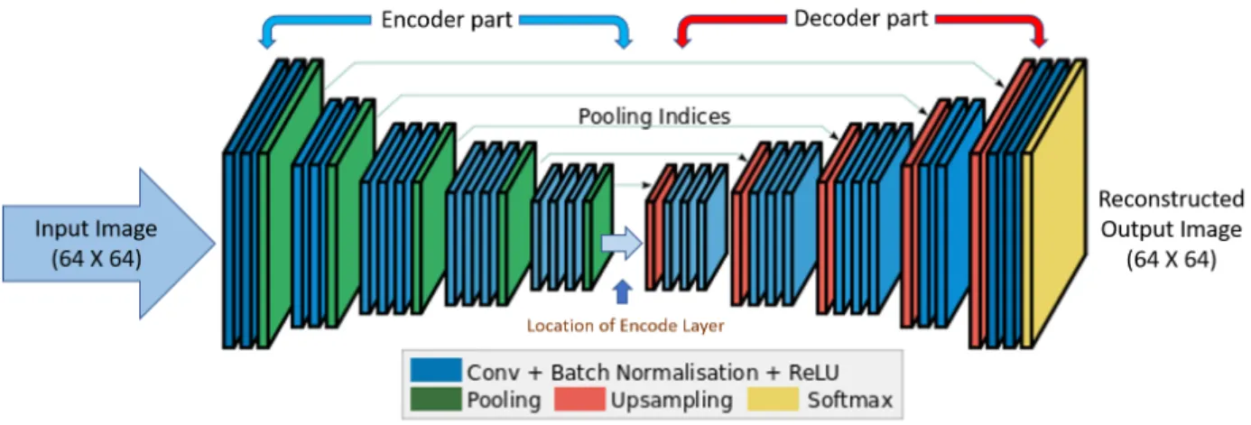
2.5 Convolutional Autoencoders
An autoencoder tries to learn the approximation to the identity function in an unsupervised manner, such that the reconstruction of the input is similar to the actual input. In unsupervised learning, only unlabeled data is used. At first glance, it seems to be trivial to learn the identity function. However, this problem becomes not so trivial anymore if we impose some constraints to the learning process such that the algorithm can discover interesting or meaningful underlying
patterns in the input data. An illustration of a typical CAE framework is given in Figure 2.7.
Figure 2.7 Illustration of a typical Convolutional Auto-Encoder architecture
For instance, in case of images, more specifically, in a natural 2D image are often correlated in terms of color. Objects in the image will also have a series of pixels that form the edges of the object. Autoencoders are algorithms that can automatically discover these correlations. Similar to principal component analysis (PCA), autoencoders can learn low-dimensional representation of the
inputs by capturing the codes within the data; in fact, the optimal solution to an autoencoder is strongly related to one found with PCA if linear activations or only a single sigmoid hidden layer are used [72]. The added advantage of autoencoders is that they can be stacked to form stacked autoencoders (SAE), another deep architecture that has a superior nonlinear modeling capacity compared to a single layer of autoencoder or PCA [73].
2.6 Training Considerations
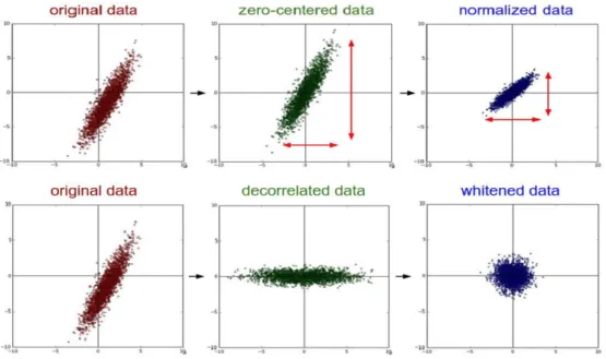
2.6.1 Data Preprocessing
Data preprocessing plays an essential part before feeding input data into a neural network. Essentially a zero-mean data is desired as an input to a neural network, as it helps in faster model training and validation. For instance, consider what happens when the input to a neuron is always
positive. In such a case, the gradients for updating the weights are always all positive or all
negative. This calls for the data to be mean. In practice, apart from making the data zero-mean and normalizing, there are other preprocessing techniques like PCA and Whitening. Figure
2.8illustrates a few data preprocessing schemes.
Figure 2.8 Data Preprocessing techniques. Illustration Courtesy: Stanford CS231n lecture
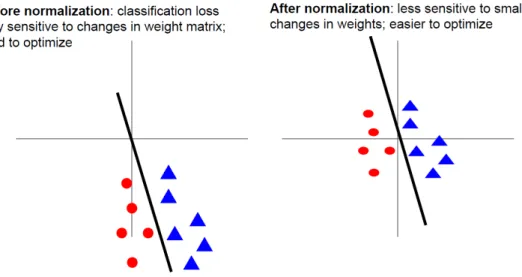
2.6.2 Batch Normalization
Introduced first in (63), Batch Normalization is a form of regularization that in essence lessens the need for other forms of regularization in a neural network. The idea behind batch normalization is to normalize the inputs of each layer in such a way that they have a mean output activation of zero and standard deviation of one (i.e, make unit gaussian activations after each convolution or pooling layer before feeding the output to the next layer). This is analogous to how the inputs to networks are standardized. A known fact is that normalizing the inputs to a network helps it learn. But a network is just a series of layers, where the output of one layer becomes the input to the next. That means we can think of any layer in a neural network as the first layer of a smaller subsequent network. Thought of as a series of neural networks feeding into each other, normalizing the output of one layer before applying the activation function, and then feed it into the following layer (sub-network), helps the learning process for the network, easier, better and faster. Figure
2.10 shows what Batch Normalization does to input data.
Figure 2.9 The idea behind performing Batch Normalization. Illustration Courtesy:
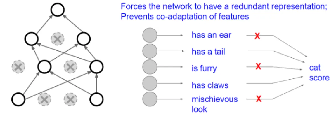
2.6.3 Regularization: Dropout
Dropout is a regularization technique for reducing overfitting in neural networks by preventing complex co-adaptations on training data. The term dropout refers to dropping out units (both hidden and visible) in a neural network. It refers to ignoring activation units (i.e. neurons) during the training phase of certain set of neurons, chosen at random. It was first introduced in (74). More technically, At each training stage, individual nodes are either dropped out of the net with
probability (1−p) or kept with probability p, so that a reduced network is left. Incoming and
outgoing edges to a dropped-out node are also removed. This is essential in a network with a lot of learning parameters. In a neural network, a fully connected layer may occupy most of the parameters, and hence, neurons develop co-dependency amongst each other during training which curbs the individual power of each neuron leading to over-fitting of training data. Dropout takes care of this issue.
Figure 2.10 Dropout takes care of over-fitting issues by randomly dropping activation
units. Illustration Courtesy: Stanford CS231n lecture notes
2.6.4 Activation Functions
Fundamentally, neural networks are layered collections of nodes, each of which receives a set of inputs and individually makes the decision whether to fire, and propagate information downstream to subsequent layers. The inputs are combined with weights and biases local to each node, which are updated by a learning algorithm in response to the observed error on training examples. This
enables patterns in data to be learned by the neural network, where the value of the weight is proportional to its importance.The weighted input data from all sources is summed to produce a single value, (called the linear combination), which is then fed into an activation function that turns it into an output signal. Conceptually, the activation function is what makes decisions: when given weighted features from some data, it indicates whether or not the features are important enough to contribute to a classification. Hence the purpose of the activation function is to introduce non-linearity into the neural network. This allows the model to generate a response variable that varies non-linearly with its explanatory variables (one where the output couldnt be reproduced from a linear combination of inputs).
For our purposes, we used the Rectified Linear Unit (ReLU) function as the activation function of choice as it has significant advantages over other choices. It not only speeds up training but also for ReLU, the gradient computation is very simple. Computation step of a ReLU is easy as well. In the context of deep neural networks, the rectifier is an activation function, defined as:
f(x) =max(0, x) (2.6)
where xis the input to a neuraon. A unit utilizing the rectifier is termed a rectified linear unit
CHAPTER 3. EXPLAINABLE AND APPLIED 2D DEEP LEARNING: BRINGING CONSISTENCY TO PLANT STRESS PHENOTYPING
Plant disease identification based on visual symptoms has predominately remained a manual exercise performed by trained pathologists, primarily due to the occurrence of confounding symp-toms. However, the manual rating process is tedious, time-consuming and suffers from inter- and intra- rater variabilities. Our work resolves such issues via introducing the concepts of explain-able deep machine learning to automate the process of plant stress identification, classification and quantification. We not only construct a very accurate model that can deliver trained pathologist-level performance, but also explains which visual symptoms it uses to make the prediction. We demonstrate that our method is applicable to a large variety of biotic and abiotic stresses as well as is transferable from one plant to another.
Current approaches for accurate identification, classification and quantification of biotic and abiotic stresses in crop research and production are predominantly visual and require specialized training. However, such techniques are hindered by subjectivity resulting from inter- and intra-rater cognitive variability. This translates to erroneous decisions and a significant waste of resources. Here, we demonstrate a machine learning framework’s ability to identify and classify a diverse set of foliar stresses in soybean [Glycine max (L.) Merr.] with remarkable accuracy. We also present an explanation mechanism using gradient-based class activation mapping that isolates the visual symptoms used by the model to make predictions. This unsupervised identification of unique visual symptoms for each stress provides a quantitative measure of stress severity, allowing for identification (type of foliar stress), classification (low, medium or high stress) and quantification (stress severity) in one framework. We reliably identified and classified several biotic (bacterial and fungal diseases) and abiotic (chemical injury and nutrient deficiency) stresses by learning from over 25,000 images. The learnt model appears to be agnostic to species and make good
predictions for other (non-Glycine max) species, demonstrating an ability of transfer learning. The availability of an explainable model that can consistently, rapidly and accurately identify and quantify foliar stresses would have significant implications in scientific research, plant breeding and crop production. The trained model could be deployed in mobile platforms (e.g., unmanned air vehicles and automated ground scouts) for rapid, large-scale scouting or as a mobile application for real-time detection of stress by farmers and researchers.
Conventional plant stress identification and classification has invariably relied on human experts identifying visual symptoms as a means of categorization (75). This process is admittedly subjective and error-prone. Computer vision and machine learning have the capability of resolving this issue and enable accurate, scalable high-throughput phenotyping.
Here, we build a deep learning model that is exceptionally accurate in identifying a large class of soybean stresses from RGB images of soybean leaves (see Figure 1). However, this type of model typically operates as a black-box predictor and requires a leap of faith to believe its predictions. In contrast, visual symptom-based manual identification provides an explanation mechanism (e.g., visible chlorosis and necrosis are symptomatic of iron deficiency chlorosis [IDC]) for disease iden-tification. The lack of explainability is endemic to most black-box models and presents a major bottleneck to their widespread acceptance (76). Here, we sought to look under the hood of the trained model to explain each identification and classification decision made. We conducted this examination by extracting the visual cues or features responsible for a particular decision and deter-mining which region of the leaf image is used by the Deep Convolutional Neural Network (DCNN) model to make a decision and whether this region is correlated with the human-identified symptoms of a particular disease. Our explanation framework is based on concepts of gradient-based class activation mapping (Grad-CAM) (69, 77), which queries each prediction of the trained model to extract visual cues (see Figure 2; also see CHAPTER 2 Section 2.4). Figure 3 illustrates this ex-planation framework with representative examples from each stress. The trained DCNN correctly identified each stress (top row) on the basis of the input image (second row). The explanation framework then (without any supervision) isolated the visual cues (i.e., most important pixels)
used by the DCNN for stress identification. These regions are highlighted in red in row 3. With statistical significance, the visual cues identified by the explanation framework correlated with the regions exhibiting visual disease symptoms, as assessed by an expert plant pathologist (see Figure 4(b)). The expert rating procedure is discussed as follows:
3.1 Severity Rating by Human Experts using a Visual Application
Multiple expert raters were also given a subset of images from our test set to rate the leaf images according to their disease severity. Thus, we obtained severity ratings based on the CNN-Grad-CAM method alongside severity metrics based on the expert raters. We used a custom built app to enable the expert raters to quickly, and efficiently mark severity measures.
Because ease of use was a priority, we chose to build a standard web application so that users could access the app immediately, on any device, without installation. We also chose not to use any particular frameworks for the front-end or back-end, instead using standard JavaScript and PHP. We used a standard MySQL database to store the marked image data. One developer created an initial prototype of the front-end in a day, which proved very useful for developing a shared vision
of the final app (see Figure3.1).
The front-end was plain HTML and JavaScript with some AJAX calls into a PHP backend. We used commonly used, well-supported technologies. We used the Raphael JS library to draw vector graphics on top of the leaf images, with simple JavaScript event handlers to simulate drawing on the image. To support touch-based mobile devices, we used the jQuery Touch Punch library to map touch events to mouse events. On the backend, the marked image data were stored by converting the path data to a JSON string and saving the data in a MySQL BLOB-type column. To track multiple users, we had the app open with an enter your user-name field. The user-name was then included in subsequent back-end requests. Because the app was used only internally and for a very brief time, we did not add any security measures against impersonation.
The web app was deployed on our group-internal web server, which runs a standard LAMP stack (Linux operating system, Apache web server, MySQL database, and PHP). After some brief
Figure 3.1 Design of the web app for expert-based foliar disease identification and severity estimation
testing, links to the application and instructions were distributed to experts to begin tagging the images. Tagging was conducted in multiple sessions during the course of one week (see Fig. S10).
The rater-based severity was calculated by marking the diseased part of the leaf and obtaining the ratio of the area (pixel count) of the marked region to the area of the entire leaf. This procedure was performed on a subset of 1000 random images extracted from the test set data (of 6576 images).
Figure 3.9 presents examples of Grad-CAM and expert-rated leaf images for each disease and
healthy cases.
3.2 Leaf Sample Collection and Data Generation
Efforts to develop the deep learning framework for the identification, classification and quan-tification of soybean stress began with the accumulation of images of stressed and healthy soybean leaflets in the field.
Figure 3.2 Illustration showing the tagging process
The labeled data needed for training were collected following a rigorous imaging protocol using
a standard camera. The imaging platform (see Figure 3.3) comprised a flat rectangular surface
covered with a dark cloth used to limit background noise. The platform was shaded by a large umbrella to ensure a consistent light source during imaging. Four leaves at a time were placed along the four corners of the platform, a color chart was placed in the center, and the leaves and chart were manually imaged using a digital camera (Canon EOS Rebel T5i, 18 megapixels). Using image processing techniques, the original images were segmented into four separate leaf images. The images were appropriately labeled as one of the eight different stress classes on the basis of the earlier field diagnoses. Each soybean stress class contained approximately 2000 leaf images with varying degrees of severity, whereas the healthy soybean class contained over 5000 images.
Over 25,000 labeled images (dataset available online) were collected to create a balanced dataset of leaflet images from healthy soybean plants and plants exhibiting eight different stresses (see
Figure 3.4). Leaflet images were taken from plants in soybean fields across the state of Iowa,
Figure 3.3 Leaf Imaging Platform
biotic (e.g., fungal and bacterial diseases) and abiotic (e.g., nutrient deficiency and chemical injury) stresses.
3.2.1 Data Collection
A total of eight different soybean stresses were selected for inclusion in the dataset, on the basis of their effects on yield loss in the state of Iowa. The eight soybean stresses included the following: bacterial blight, bacterial pustule, Septoria brown spot, sudden death syndrome (SDS), frog-eye leaf spot, herbicide injury, potassium deficiency, and iron deficiency chlorosis (IDC) (78). Healthy soybean leaflets were also collected to serve as a ground truth for the machine learning model for the successful differentiation of healthy and stressed leaves. First, various soybean fields in central Iowa associated with Iowa State University were scouted for the desired plant stresses. Entire plant samples were collected directly from the fields and taken to the Plant and Insect Diagnostic Clinic at Iowa State for official diagnosis by expert plant pathologists; for more information and
online access, please follow this link to the online Plant and Insect Diagnostic Clinic. The exact
locations of the sampled soybean plants were recorded at that time. After the stress identities were confirmed by the Plant and Insect Diagnostic Clinic, the desired fields were revisited. Individual
Potassium Deficiency Herbicide Injury Frogeye Leaf Spot FUNGAL Bacterial Blight Bacterial Pustule Sudden Death Syndrome Septoria Brown Spot Chemical Injury BIOTIC BIOTIC Fungal Bacterial Nutrient Deficiency Iron Deficiency Chlorosis PLANT STRESSES BIOTIC ABIOTIC Symptoms: large irregularly shaped blotches
of necrosis between the veins; Area of appearance: mid and upper leaves in a canopy;
Mistaken with: Brown stem rot due to similar characteristic symptoms of
interveinal chlorosis
Symptoms:lesions are circular with gray to light brown center with dark reddish
brown margins. Lesion diameter range from 1-5 mm; Area of appearance: leaves in upper canopy.
Symptoms: lesions are irregular-shaped and dark brown in color. Adjacent lesions grow together and form larger blotches which are darker than the lesions of other diseases; Area of appearance: leaves in lower canopy. Leaves quickly turn yellow and drop; Mistaken with:
Bacterial blight.
Symptoms: lesions are small and surrounded by
yellow halo and some lesions have pin-point brown spots. Small pustule lesions are located on the underside
of the leaf; Area of appearance: leaves in
mid to upper canopy;
Mistaken with: bacterial blight; however, BP does not result in tattering of
leaves.
Symptoms: lesions are angular shaped with reddish brown centers. Margins of disease spot surrounded by yellow halos. Lesions coalesce into larger irregularly shaped area that fall out;
Area of appearance: leaves in mid to upper canopy; Mistaken with: Septoria brown spot.
Symptoms: yellowing of interveinal areas of leaves, while the veins remain green. Later on small brown specks on affected leaves; Area of appearance: usually
on young leaves in a canopy.
Symptoms: continuous yellow margin at the tip of the leaf. Yellowing is followed by necrosis;
Area of appearance:
lower and older leaves in a canopy.
Symptoms: small brown specking to severe bronzing and bleaching;
Area of appearance: leaves that come in contact with the chemical.
Figure 3.4 Schematic illustration of foliar plant stresses in soybean grouped into two
ma-jor categories, biotic (bacterial and fungal) and abiotic (nutrient deficiency and chemical injury) stress. The images were used to develop the DCNN for the
fol-lowing eight stresses: bacterial blight (Pseudomonas savastanoi pv. glycinea),
bacterial pustule (Xanthomonas axonopodis pv. glycines), sudden death
syn-drome (SDS,Fusarium virguliforme), Septoria brown spot (Septoria glycines),
frogeye leaf spot (Cercospora sojina), IDC, potassium deficiency and herbicide
injury. For each stress, information such as symptom descriptors, areas of ap-pearance and most commonly mistaken stresses that exhibit similar symptoms are listed. These particular foliar stresses were chosen because of their large economic impact on agriculture and confounding symptoms.
soybean leaflets exposed to a range of different severity levels were then identified and collected manually through destructive sampling. Diseases such as frog-eye leaf spot, potassium deficiency, bacterial pustule and bacterial blight were present at low to medium intensity. The leaflets were placed into designated bags and transported to the imaging platform on-site.
3.2.2 Data Preparation and Generation
The dataset for training, validation and testing was prepared in the following manner: First, the images of the leaves were segmented out from the raw images and reshaped into images of pixel size 64X64 [(height) X (width)] to generate images for training the deep neural network efficiently. We used 4174 images for healthy leaves, 1511 images for bacterial blight, 1237 images for brown spot, 1096 images for frogeye spot, 1311 images for herbicide injury, 1834 images for IDC, 2182 images for potassium deficiency, 1634 images for bacterial pustule and 1228 images for SDS, i.e., a
total of 16207 clean images. Refer to Figure 3.4 that show example images for each class, where
Bacterial Blight Injury was designated as class 0, Brown Spot as class 1, Frogeye Leaf Spot as class 2, Herbicide Injury as class 4, Iron Deficiency Chlorosis as class 5, Potassium Deficiency Syndrome as class 6, Bacterial Pustule Injury as class 7, Sudden Death Syndrome as class 8 and finally healthy leaves as class 3.
A data augmentation scheme was adopted to increase the size of the dataset. To perform data augmentation, we used 1096 images for each of the disease classes and 2192 from the healthy class. The following augmentations were conducted: horizontal flip, vertical flip, 90 degree clockwise (CW) rotation, 180 degree CW rotation and 270 degree CW rotation, (see supplementary). We generated a total of 65760 images, which were then divided into training, validation and test sets
in a 7:2:1 proportion. Refer to Figure 3.5for an illustration of the data augmentation scheme.
3.3 Deep CNN Model and Explanation Framework
We built a deep convolutional neural network- (DCNN-) based supervised classification frame-work to identify and classify stresses (Figure 2 (a) and (b)). DCNNs have shown an extraordinary ability (1, 2, 3, 4, 5, 79, 80) to efficiently extract complex features from images and function as a
classification technique when provided with sufficient data (see Section3.3.2). The exhibited
accu-racy is especially promising, given the multiplicity of similar and confounding symptoms between the stresses in single crop species (see Figure 1). We associate this classification ability with the hierarchical nature of this model (81), which is able to learn features of features from data without the time-consuming hand-crafting of features (see CHAPTER 2 Section 2.3). Upon classification inference, we use the Grad-CAM algorithm (69) to generate heat maps on a test leaf image that signifies the leaf region the DCNN model is focusing on to perform the classification.
3.3.1 Network Parameters
The DCNN architecture (shown in Figure 2) consists of 5 convolutional layers (128 feature maps of size 3X3 for each layer), 4 pooling layers (down sampling by 2X2 max-pooling), 4 batch normalization layers and 2 fully connected (FC) layers with 500 and 100 hidden units each,
sequen-tially. Training was performed on a total of 53,265 samples (with an additional 5,919 validation
samples), and testing was performed on 6,576 samples. The learning rate was maintained at 0.1.
The first convolutional layer maps the 3 bands (RGB) in the input image to 128 feature maps by using a 3X3 kernel function. Subsequent max-pooling decreases the dimensions of the image. This step is performed by taking the maximum value in a window that is passed over the image. The stride here is the default stride, i.e., 2, which means that the window is moved 2 pixels at a time. This decrease in image dimension reduces computation complexity and time, thereby allowing the model to fit in the memory available from the graphics processing unit (GPU) (82).
3.3.2 Training the DCNN
Our designed architecture initially had close to 3 million learning parameters, which was reduced
to ˜900,000 while the same level of prediction accuracy was maintained. Although deep neural
networks with a large number of learning parameters are very powerful architectures, overfitting becomes a severe problem in these cases. Large networks such as these are also slow to train, thus making it more difficult to address overfitting issues by combining the predictions of many large neural networks during the testing phase. Adding Dropout layers can usually solve such overfitting issues. The idea behind adding dropout layers is to randomly drop units along with their connections from the neural network during training (74). The percentage of dropouts used in our model is depicted in Figure 2 of the main text. The last FC layer after the final dropout layer gives the prediction for the class to which the input image belongs. After every convolutional layer, batch normalization was performed to remove internal covariate shift (63). The network was trained for approximately 100 epochs on the 53,265-image training set to reach the desired accuracy. The cross-entropy (categorical) loss (or cost) function along with the Adam optimizer (83) was used to minimize the error. Adam was chosen as the optimizer primarily because it requires minimal tuning of its internal hyper parameters. All other hyper parameters mentioned above have been cross-validated and chosen on the basis of repeated experiments to achieve the
best possible prediction accuracy. Figure 3.6 shows how the prediction accuracy varies with the
availability of training data, and suggests that performance has reached an asymptotic value.
3.4 Results
3.4.1 Disease Classification and Identification
While Figure 3 presents the qualitative results of deploying the trained DCNN for disease detection and classification, Figure 4 and Figure 5 detail the quantitative results over all test images. We found a high overall classification accuracy (94%) using a large and diverse dataset of unseen test examples (approximately 6000 images, i.e., approximately 600 examples per foliar stress).
Figure 3.6 Variation of test accuracy w.r.t. the increasing size of training data
The confusion matrix revealed that erroneous predictions were predominantly due to confounding disease symptoms that cause confusion even for expert raters (Figure 4). For example, the highest confusion (17.6% of bacterial pustule test images predicted as bacterial blight and 11.6% of bacterial blight test images predicted as bacterial pustule) occurred between bacterial blight and bacterial pustule; discriminating between these two diseases is challenging even for expert plant pathologists (84).
3.4.2 Symptom Explanation and Severity Quantification
In conventional disease-scouting scenarios, the ratings of even the same expert rater may change depending on various factors (intra-rater variability), such as illumination and human fatigue. Moreover, different human raters often tend to disagree (inter-rater variability), owing to the sub-jective quantification of the extent of symptoms expressed on a leaf (75, 85). In contrast, the trained
Figure 3.7 (a) DCNN architecture used. (b) Prediction Explanation Phase. The concept of gradient-based class activation mapping (Grad-CAM) was applied to auto-matically visualize image features used by the DCNN model when making a classification decision.
DCNN provides a consistent approach for severity estimation. Specifically, the spatial spread of the automatically identified symptoms allows for estimation of the severity of the classified disease in each leaflet. We computed the severity as the area fraction of identified symptoms and compared it with the severity estimated by an expert human rater. While the algorithm identified symptoms extremely precisely (at a pixel level), the expert human rater estimate was much more qualita-tive. This qualitative estimate was made by comparing the predicted severity rating to disease severity data collected from expert marking of symptoms challenging, primarily because of large inter-rater variability, as shown in Figure 4 (b). The decidedly more qualitative approach for the determination of disease spread by human experts resulted in severity values that were consistently larger than the precise machine learning-based annotations. We used a calibration process to map each human expert-annotated severity rating to a reference rating to make inter-rater comparison possible, thus rationally permitting the comparison of disease severity predictions between human
Figure 3.8 (a) This confusion matrix shows the stress classification results of the DCNN model for eight different stresses and healthy leaves. The overall classification
accuracy of the model is 94%. The greatest confusion among stresses was
found among bacterial blight, bacterial pustule, and Septoria brown spot. A reasonable explanation for these higher failure rates can be attributed to the similarities in symptom expression among these stresses.(b) is a scatter plot comparing the severity ratings of the same images between two raters for four stresses (IDC, SDS, potassium deficiency and Septoria brown spot) that were
pooled and solid red line is the 45o line. The results indicated high inter-rater
variability between experienced raters, especially as the stress severity of leaf images increase.
c) shows a comparison of the machine learning-based ratings and human ratings based on a typical discretized severity scale (0-15%: resistant, 15-30%: moderately resistant, 30-45%: moderately sus-ceptible, 45-75%: sussus-ceptible, and 75-100%: highly susceptible). Furthermore, these rating results demonstrated the efficacy of the DCNN-based severity estimation framework, which identifies the disease symptoms in a completely unsupervised manner. We observed that the few deviations in these results were primarily due to the low quality of the corresponding images, which exhibited
Figure 3.9 This table presents leaf image examples for each soybean stress identified and classified by the DCNN model. The Grad-CAM framework was applied to highlight regions of interest (symptoms) extracted by the DCNN model. These automatically extracted symptoms were compared against versions of images with symptoms that were marked manually by expert raters.
3.4.2.1 Calibration Procedure
The machine learned severity, rim/c, performed quite well with many leaf images and was
con-sistent with the user ratings,ri
u. However, in some cases,rim/c provided a lower estimate of severity
than the expert-based severity because human expert-based markings tended to be much coarser. In effect, typically all regions surrounding an affected region on a particular affected leaf are high-lighted. However, the machine learning model via Grad-CAM is often too specific (at a pixel-level resolution) and highlights only the most important regions for a particular class to be activated. Therefore, a calibration process is required to achieve a uniform scale for machine learning-based severity and expert-based severity.