UC Santa Barbara Electronic Theses and Dissertations
Title
ADCN: An Anisotropic Density-Based Clustering Algorithm for Discovering Spatial Point Patterns with Noise
Permalink https://escholarship.org/uc/item/3np9r4zb Author Mai, Gengchen Publication Date 2017 Peer reviewed|Thesis/dissertation
ADCN: An Anisotropic Density-Based Clustering
Algorithm for Discovering Spatial Point Patterns
with Noise
A dissertation submitted in partial satisfaction of the requirements for the degree
Master of Art in Geography by Gengchen Mai Committee in charge:
Professor Krzysztof Janowicz, Chair Professor Werner Kuhn
Professor Kostas Goulias
Professor Werner Kuhn
Professor Kostas Goulias
Professor Krzysztof Janowicz, Committee Chair
Point Patterns with Noise
Copyright c 2018 by
I would like to thank the members of my Master’s committee for their great sugges-tions and guidance throughout this thesis. I would like to thank my adviser, Professor Krzysztof (Jano) Janowicz, for his very strong support during every stage of my life as a graduate student. The last two years have been very difficult for me. The loss of family members nearly put me in a hole while Jano and other members from STKO Lab helped me to get through this extremely difficult time. Nonetheless, these two years make me become very enthusiastic about research and it is Jano who makes me an independent researcher. I would like to thank Yingjie Hu and Song Gao for helping me build up the research framework of this thesis and offering me many useful suggestions. I would like to thank all of my STKO colleagues for their companionship and friendship. I would like to thank Professor Daniel Montello and Professor Martin Raubal for inspiring me during the initial stage of this research. Last, but most importantly, I would like to thank my family, especially my mother, for their unconditional love, support and companion during the darker times of my life.
Education
2020 Ph.D. in Geography (Expected), University of California, Santa Barbara.
2017 M.A. in Geography (Expected), University of California, Santa Bar-bara.
2015 B.S. in Geographic Information System, Wuhan University.
Awards
• Travel Grants
2017 The Jack & Laura Dangermond Travel Scholarship for ACM SIGSPATIAL 2017 2017 The Jack & Laura Dangermond Travel Scholarship for AAG 2017
2016 The Jack & Laura Dangermond Travel Scholarship for ACM SIGSPATIAL 2016 2016 The Jack & Laura Dangermond Travel Scholarship for GIScience 2016
2016 NSF Student Fellowship for RW2016
2016 The Jack & Laura Dangermond Travel Scholarship for RW2016 2016 The Jack & Laura Dangermond Travel Scholarship for AAG 2016
• Fellowships, Scholarships, and Awards
2017 The 1st Place Best Paper Award at AAG 2017 GIS Special Group Student Paper Competition for ”Beyond Coordinates: Incorporating Geographic Knowledge into Geocoding Services Using Linked Open Data” (co-author)
2015 UCSB Geography Doctoral Scholars Fellowship 2015 Outstanding Undergraduate of Wuhan University 2013 China National Fellowship
2013 First-class scholarship and Merit Student of School of Resource and Environmental Sciences, Wuhan University
2012 China National Fellowship
2012 First-class scholarship and Merit Student of School of Resource and Environmental Sciences, Wuhan University
Publications
• Book Chapters
1. Song Gao, Gengchen Mai. (2017) Mobile GIS and Location-Based Services. In Bo Huang, Thomas J. Cova, and Ming-Hsiang Tsou et al.(Eds): Comprehensive Geographic Information Systems, Elsevier. Oxford, UK.
• Peer-reviewed Journal Articles
1. Gengchen Mai, Krzysztof Janowicz, Yingjie Hu, Song Gao. ADCN: An Anisotropic Density-Based Clustering Algorithm for Discovering Spatial Point Patterns with Noise. Transactions in GIS, in press. DOI:10.1111/tgis.12313
2. Shiliang Su, Yaping Wang, Fanghan Luo, Gengchen Mai, Jian Pu. Peri-urban vegetated landscape pattern changes in relation to socioeconomic development. Eco-logical Indicators 46 (2014) 477486.
3. Shiliang Su, Yina Hu, Fanghan Luo, Gengchen Mai, Yaping Wang. Farmland fragmentation due to anthropogenic activity in rapidly developing region. Agricul-tural Systems 131 (2014) 8793.
4. Rui Xiao, Shiliang Su, Gengchen Mai, Zhonghao Zhang, Chenxue Yang. Quan-tifying determinants of cash crop expansion and their relative effects using logistic regression modeling and variance partitioning. International Journal of Applied Earth Observation and Geoinformation 34 (2015) 258263.
• Conference Papers
1. Bo Yan, Krzysztof Janowicz,Gengchen Mai, Song Gao. From ITDL to Place2Vec - Reasoning About Place Type Similarity and Relatedness by Learning Embeddings From Augmented Spatial Contexts, In: Proceedings of the 25th International Con-ference on Advances in Geographic Information Systems (ACM SIGSPATIAL 2017), November 7 - 10, 2017, Redondo Beach, California, USA. (Full paper accepted) 2. Blake Regalia, Krzysztof Janowicz, Gengchen Mai. Phuzzy.link: A
SPARQL-powered Client-Sided Extensible Semantic Web Browser, In: Proceedings of 3rd International Workshop on Visualization and Interaction for Ontologies and Linked Data (VOILA 2017) co-located with ISWC 2017, October 22, 2017, Vienna, Austria. (Full paper accepted)
ference on Advances in Geographic Information Systems (ACM SIGSPATIAL 2016), October 31 - November 3, 2016, San Francisco Bay Area, California, USA. (Short paper accepted)
4. Gengchen Mai, Krzysztof Janowicz, Yingjie Hu, Grant McKenzie. A Linked
Data Driven Visual Interface for the Multi-Perspective Exploration of Data Across Repositories, In: Proceedings of 2nd International Workshop on Visualization and Interaction for Ontologies and Linked Data (VOILA 2016) co-located with ISWC 2016, October 17, 2016, Kobe, Japan. (Full paper accepted)
5. Song Gao, Rui Zhu, Gengchen Mai. Identifying Local Spatiotemporal Autocor-relation Patterns of Taxi Pick-ups and Drop-offs, In: Proceedings of the 9th Inter-national Conference on Geographic Information Science, September 27 - 30, 2016, Montreal, Canada. (Short paper accepted)
6. Krzysztof Janowicz, Yingjie Hu, Grant McKenzie, Song Gao, Blake Regalia,Gengchen Mai, Rui Zhu, Benjamin Adams, and Kerry Taylor. Moon Landing or Safari? A Study of Systematic Errors and Their Causes in Geographic Linked Data, In: Pro-ceedings of the 9th International Conference on Geographic Information Science, September 27 - 30, 2016, Montreal, Canada. (Full paper accepted)
ADCN: An Anisotropic Density-Based Clustering Algorithm for Discovering Spatial Point Patterns with Noise
by Gengchen Mai
Density-based clustering algorithms such as DBSCAN have been widely used for spa-tial knowledge discovery as they offer several key advantages compared to other clustering algorithms. They can discover clusters with arbitrary shapes, are robust to noise and do not require prior knowledge (or estimation) of the number of clusters. The idea of using a scan circle centered at each point with a search radius Eps to find at least MinPts
points as a criterion for deriving local density is easily understandable and sufficient for exploring isotropic spatial point patterns. However, there are many cases that cannot be adequately captured this way, particularly if they involve linear features or shapes with a continuously changing density such as a spiral. In such cases, DBSCAN tends to either create an increasing number of small clusters or add noise points into large clus-ters. Therefore, in this paper, we propose a novel anisotropic density-based clustering algorithm (ADCN). To motivate our work, we introduce synthetic and real-world cases that cannot be sufficiently handled by DBSCAN (and OPTICS). We then present our clustering algorithm and test it with a wide range of cases. We demonstrate that our algorithm can perform as equally well as DBSCAN in cases that do not explicitly benefit from an anisotropic perspective and that it outperforms DBSCAN in cases that do. We show that our approach has the same time complexity as DBSCAN and OPTICS, namely O(n log n) when using a spatial index and O(n2) otherwise. We provide an implementa-tion and test the runtime over multiple cases. Finally, we apply DBSCAN, OPTICS, and
six cities. Visual comparison shows that, comparing to DBSCAN and OPTICS, ADCN is inclined to extract AOIs with linear shapes which follow the underline road networks. ADCN also turns out to connect clusters when the spatial distribution of them shows similar directions.
Curriculum Vitae v
Abstract viii
1 Introduction and Motivation 1
2 Related Work 6
2.1 Density-based Clustering Algorithm . . . 7
2.2 Anisotropicity . . . 8
2.3 Clustering Comparison Indexes . . . 11
2.4 Research Question . . . 16
3 Anisotropic Density-based Clustering with Noise (ADCN) 17 3.1 Anisotropic Perspective on Local Density . . . 17
3.2 Anisotropic Density-Based Clusters . . . 19
3.3 ADCN Algorithms . . . 24
4 Experiments and Performance Evaluation 29 4.1 Experiment Designs . . . 30
4.2 Test Environment . . . 31
4.3 Evaluation of Clustering Quality . . . 35
4.4 Evaluation of Clustering Efficiency . . . 38
5 Real World Application 44 5.1 Data Preprocessing and Clustering . . . 45
5.2 Constructing AOI from point clusters using chi-shape algorithm . . . 46
6 Conclusion and Future Work 56 6.1 Conclusion . . . 56
6.2 Future Work . . . 58
Introduction and Motivation
Cluster analysis is a key component of modern knowledge discovery whose objective is to maximize the intra-cluster similarity while minimizing the inter-cluster similarity at the same time. The objects as a basic analytic unit can be anything whose attributes can be quantified, including geographic footprints from social media platforms [1, 2, 3, 4], human activity traces [5], places, documents [6, 7], and so on. Because of the domain independent definition of ”objects” in cluster analysis, it has been widely applied to data analysis tasks from many research disciplines and is widely considered a key technique used for reducing dimensionality, identifying prototypes, cleansing noise, determining core regions, and segmentation.
A wide range of clustering algorithms have been proposed and implemented over the last decades to achieve the objective of clustering analysis from different perspectives. Common examples include DBSCAN [8], OPTICS [9], K-means [10], K-medians [11], ASCDT [12], and Mean Shift [13]. These techniques often yield different clustering re-sults for the same data due to differences in the underlying understanding of what should be clustered and how. K-means and K-medians, for instance, first find representatives for each cluster and update them as well as the cluster memberships of each object by
minimizing the distance between cluster representatives and other objects in the same cluster. Hence, detected clusters will have spherical shapes with similar sizes. Both tech-niques also have no notion of noise as each object belongs to some cluster. In contrast, DBSCAN, OPTICS or other density-based clustering algorithms try to find clusters in which the density of objects is larger than a threshold. The resulting clusters can have arbitrary shapes and varied sizes but with similar or homogenous object densities. Noise is defined as objects in low density regions. Delaunay triangulation-based clustering algorithms, like ASCDT [12], find clusters based on spatial proximity between objects defined via Delaunay triangulations. due to different distance metrics (Delaunay trian-gulation based distance metrics), ASCDT can discover clusters of complicated shapes and non-homogeneous densities in a spatial database. However, Delaunay triangulation based clustering algorithms cannot be easily scaled up to a large spatial dataset because of the high time complexity for computing the triangulation.
Many clustering algorithms including all algorithms we discussed above depend on
distance as their main criterion [14]. They assumeisotropic second-order effects (i.e., spa-tial dependence) among spaspa-tial objects thereby implying that the magnitude of similarity and interaction between two objects mostly depends on their distance. However, the gen-esis of many geographic phenomena demonstrates clearanisotropic spatial processes. As for ecological and geological features, such as the spatial distribution of rocks [15], soil [16], and airborne pollution [17], their spatial patterns vary in direction [18]. Similarly, data about urban dynamics from social media, the census, transportation studies, and so forth, are highly restricted and defined by the layout of urban spaces, and thus show clear variance along directions. To give a concrete example, geo-tagged images be it in the city or the great outdoors, show clear directional patterns due to roads, hiking trails, or simply for the fact that they originate from human, goal-directed trajectories. Isotropic clustering algorithms such as DBSCAN have difficulties dealing with the resulting point
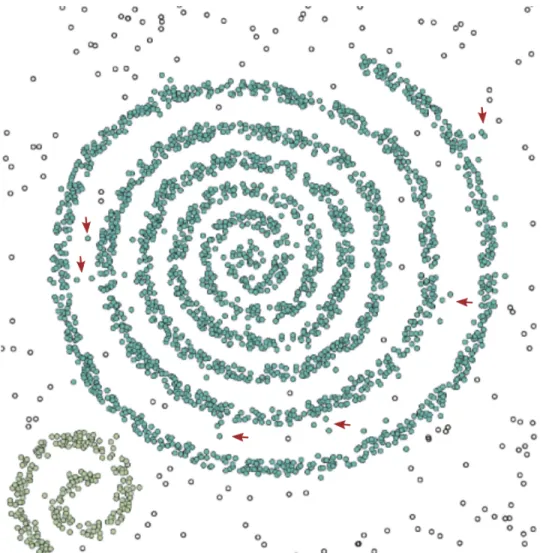
patterns and either fail to eliminate noise or do so at the expense of introducing many small clusters. One such example is depicted in Figure 1.1. Due to the changing den-sity, algorithms such as DBSCAN will classify some noise, i.e., points between the spiral arms, as being part of the cluster. To address this problem, we propose an anisotropic density-based clustering algorithm.
Figure 1.1: A spiral pattern clustered using DBSCAN. Some noise points are indicated by red arrows.
More specifically, the research contributions of this paper are as follows:
• We introduce an anisotropic density-based clustering algorithm (ADCN 1). While 1This paper is based on the short paper [19] and the paper [20]. It also adds an open source
imple-the algorithm differs in imple-the underlying assumptions, it uses imple-the same two parameters as DBSCAN, namely Eps and MinPts, thereby providing an intuitive explanation and integration into existing workflows.
• We motivate the need for such algorithm by showing 12 synthetic and 8 real-world use cases and each with 3 different noise definitions modeled as buffers that generate a total of 60 test cases.
• We demonstrate that ADCN performs as well as DBSCAN (and OPTICS) for isotropic cases but outperforms both algorithms in cases that benefit from an anisotropic perspective.
• We argue that ADCN has the same time complexity as DBSCAN and OPTICS, namely O(n log n) when using a spatial index and O(n2) otherwise.
• We provide an implementation for ADCN and apply it to the use cases to demon-strate the runtime behavior of our algorithm. As ADCN has to compute whether a point is within an ellipse instead of merely relying on the radius of the scan circle, its runtime is slower than DBSCAN while remaining comparable to OPTICS. We discuss how the runtime difference can be reduced by using a spatial index and by testing the radius case first.
• Finally, we apply ADCN, DBSCAN, and OPTICS to a 2013-2014 Flickr geotagged photo dataset from six cities to extract urban areas of interest (AOI). Although there is noground truthin this task, by comparing the extracted AOIs from different algorithms, we are able to show that the AOIs extracted from ADCN tend to have linear shapes that follow road networks. We perform this analysis to show that mentation of ADCN, a test environment, as well as new evaluation results on a larger sample.
ADCN does not only yield different results for test cases but that these differences have impact on cluster formation using large scale real-world data.
The remainder of the paper is structured as follows. First, in Chapter 2, we discuss related work including variants of DBSCAN, anisotropicity of spatial point patterns, and clustering comparison indexes. Next, we introduce ADCN and discuss two potential realizations of measuring anisotropicity in Chapter 3. In Chapter 4, several experiments are described to demonstrate the effectiveness of ADCN. Use cases, the development of a test environment, and a performance evaluation of ADCN are presented in Chapter 4. Next, in Chapter 5, ADCN, DBSCAN and OPTICS are applied to a real-world application, namely urban AOI extraction, to show the advantages of ADCN. Finally, in Chapter 6, we conclude our work and point to directions for future work.
Related Work
Clustering algorithms can be classified into several categories, including but not limited to partitioning, hierarchical, density-based, graph-based, and grid-based approaches [21, 12]. Each of these categories contains several well known clustering algorithms with their specific pros and cons. Partitioning clustering, such as K-Means, PAM [22] and CLARANS [23], aims at finding mutually exclusive clusters of spherical shapes. It has difficulties in handling clusters of different sizes and shapes. Hierarchical clustering, such as single-link and complete-link, approaches build a hierarchical tree of clusters. When there are some erroneous merges or splits during the hierarchical tree construction process, they cannot be corrected later. Grid-based clustering segments the data space into grid cells [24]. That means it will suffer from the common drawbacks of image operations. Here we focus on the density-based approaches and we will review them below.
2.1
Density-based Clustering Algorithm
Density-based clustering algorithms are widely used in big geo-data mining and analy-sis tasks, like generating polygons from a set of points [25, 26, 27], discovering urban areas of interest [2], revealing vague cognitive regions [3], detecting human mobility patterns [28, 29, 30, 31], and identifying animal mobility patterns [32].
Density-based clustering algorithms, such as DBSCAN [8], OPTICS [9], DENCLUE [33], have many advantages over other approaches. Figure 2.1 shows the best clustering results from K-Means and DBSCAN based on one clustering result comparison index 1. By comparing the clustering results between these two algorithms, we can observe sev-eral advantages of DBSCAN including: 1) the ability to discover clusters with arbitrary shapes; 2) robustness to noise; and 3) no requirement to pre-define the number of clus-ters. While DBSCAN remains the most popular density-based clustering method, many related algorithms have been proposed to compensate for some of its limitations. Most of them, such as OPTICS [9] and VDBSCAN [34], address problems arising from density variations within clusters. Others, such as ST-DBSCAN [35], add a temporal dimension which means the objects within each extracted cluster are approximated to each other spatio-temporally. However, an additional temporal parameter is necessary. GDBSCAN [36] extends DBSCAN to include non-spatial attributes into clustering and enables the clustering of high dimensional data. NET-DBSCAN [37] revises DBSCAN for network data by redefining the distance matrics based on network structures. To improve the computational efficiency, algorithms such as IDBSCAN [38] and KIDBSCAN [24] have been proposed.
(a) K-Means (b) DBSCAN Figure 2.1: Clustering result comparison between K-means and DBSCAN.
2.2
Anisotropicity
All of these algorithms use distance as the major clustering criterion. They assume that the observed spatial patterns are isotropic, i.e., that intensity dose not vary by direction. For example, DBSCAN uses a scan circle with anEps radius centered at each point to evaluate the local density around the corresponding point. A cluster is created and expanded as long as the number of points inside this circle (Eps-neigborhood) is larger than MinPts. Consequently, DBSCAN does not consider the spatial distribution of the Eps-neigborhood which poses problems for linear patterns.
Some clustering algorithms do consider local directions. However, most of these so-call direction-based clustering techniques use spatial data which have a pre-defined local direction, e.g., trajectory data. The local direction of one point is pre-defined as the direction of the vector which is part of the trajectories with the corresponding point as its origination or destination. DEN [39] is one direction-based clustering method which uses a grid data structure to group trajectories by moving directions. PDC+ [40] is another trajectory specific DBSCAN variant that includes the direction per point.
DB-SMoT [41] includes both the direction and temporal information of GPS trajectories from fishing vessel into the clustering process. Although all of these three direction-based clustering algorithms incorporate local direction as one of the clustering criteria, they can be applied to only trajectories data.
Many spatial data sets do not have predefined local direction information which can show the moving directions of objects under study. However, because the underline spatial point process is anisotropic, the spatial patterns shown by the cumulative spatial datasets generated from this process varies in direction and demonstrates the direction information of underline spatial point process. For example, geotagged social media data, like Foursquare check-in data, geotagged tweets, reflects human dynamic mobilities in/across the urban area which are highly restricted by the urban spatial structure (road networks). So these user-generated geospatial data show a spatial pattern distributed along road networks. Figure 2.2 shows the spatial distribution of geotagged tweets during April 2014 in California, USA. The major road networks in California is clearly revealed from these tweets.
Anisotropicity [18] describes the variation of directions in spatial point processes in contrast to isotropicity. It is another way to describe intensity variation in spatial point process other than first- and second-order effects. Anisotropicity has been studied in the context of interpolation where a spatially continuous phenomenon is measured, such as directional variogram [17] and different modifications of Kriging methods based on local anisotropicity [42, 43, 44]. In this work we focus on anisotropicity of spatial point processes. Researchers studiedanisotropicity of spatial point processes from a theoretical perspective by analyzing their realizations such as detecting anisotropy in spatial point patterns [45] and estimating geometric anisotropic spatial point patterns [46, 47]. Here, we study anisotropicity in the context of density-based clustering algorithms.
Figure 2.2: Geo-tagged tweets during April, 2014 in California, USA
in order to obtain good results for crack detection, an anisotropic clustering algorithm [48] has been proposed to revise DBSCAN by changing the distance metric to geodesic distance. QUAC [49] demonstrates another anisotropic clustering algorithm which does not make an isotropic assumption. It takes the advantages of anisotropic Gaussian kernels to adapt to local data shapes and scales and prevents singularities from occurring by fitting the Gaussian mixture model (GMM). QUAC emphasizes the limitation of an isotropic assumption and highlights the power of anisotropic clustering. However, due to the use of anisotropic Gaussian kernels, QUAC can only detect clusters which have ellipsoid shapes. Each cluster derived from QUAC will have a major direction. In real-world cases, spatial pattern will show arbitrary shapes. Even more, the local direction is not necessary the same between and even within clusters. Instead, it is reasonable to assume that local direction can change continuously in different parts of the same cluster. From the above discussion of different clustering algorithms, it is clear that an
isotropic assumption may be inappropriate for many geographic phenomena. On top of local density, it is necessary to consider local direction during the clustering process. This local direction is not necessary the same for one cluster. Instead, it is reasonable that the local direction is changing continuously in different parts of one cluster.
2.3
Clustering Comparison Indexes
Evaluating the clustering result is the final and important step in cluster analysis. In general, clustering evaluation methods can be divided into two categories: intrinsic and extrinsic [50]. Given a similarity metric between objects, intrinsic clustering evaluation methods compute how similar objects in one cluster are to each other, and how dissimilar to objects from different clusters they are. In other words, intrinsic evaluation assesses the goodness of a clustering by computing how well the clusters are separated [21]. When a
ground truth/gold standard is available, extrinsic clustering evaluation methods will play a role by comparing the output from one clustering algorithm to theground truth. Here,
ground truth/gold standard is the ideal clustering result obtained from human experts, prior knowledge, convention, or otherwise. In this work, we focus on extrinsic methods.
Many clustering comparison indexes have been proposed for extrinsic clustering eval-uation. Marina et al. [51], Nguyen Xuan et al. [52], and more recent Jiawei et al. [21] have presented a review of these clustering comparison indexes. Traditionally, many re-searchers agree that measures for comparing clusterings can be classified aspair-counting based measures, set-matching based measures, and information theoretic measures. But recently, new measures have been proposed which cannot be classified into these three categories, such as clustering measure using density profile [53], Mallows distance based measures [54], and transportation distance based measure [55]. We will briefly discuss them below.
Pair-counting based measures count pairs of items on which two clusterings agree or disagree (one clustering result and the ground truth), such as Wallace index [56], FowlkesMallows index [57], Rand index [58], Adjusted Rand index [59], Jaccard index [60], Mirkin index [61]. In this work, we use Rand index to evaluate our proposed clustering algorithm ADCN and we will discuss it in detail in Section 4.
Set matching based measures match the ‘best’ clusters between two clustering results based on the number of shared objects, such as Clustering Error [62], the asymmetric metric proposed by Larsen et al. [63], and the metric proposed by van Dongen et al. [64]. A problem withSet matching based measures is that the criteria it uses completely ignore the information of the ”unmatched” part of each cluster [62].
Information theoretic measures, which are based on information theory, measure the amount of mutual information shared by two clustering results via the number of objects they agree, such as Mutual Information [65], Normalize Mutual Information with different normalize methods [66, 67, 68, 69], Adjusted-for-Chance MI [52], Unnormalized distance measures [66, 62], and Normalized distance measures [68, 52]. In this work, we utilize Normalize Mutual Information from Strehl et al. [67] which we will discuss in detail in Section 4 in addition to Rand index to ensure that we use measures from different families.
All the clustering comparison measure we mentioned above are purely from a statistic perspective and treat clusterings as partitions of atoms. They compare clusterings based on the memberships of objects to different clusters. That means that an object clustered into any other clusters will be treated as equally wrong. But Zhou et al. [54], Bae et al. [53], Coen et al. [55] made an argument that miss classifying one object to different clusters will have different effects on the clustering similarity judgement. Figure 2.3 illustrates such idea. Figure 2.3 (a) shows the ground truth in which there are three clusters A, B, and C. Figure 2.3 (b) and (c) shows the clustering result of Clustering
X and Y in which 10 objects/points in Cluster B’(C”) have been miss classified into Cluster A’(A”). Zhou et al. [54], Bae et al. [53], Coen et al. [55] argued that existing clustering comparison measures (the traditional three categories we discussed above) will yield the same similarity between the ground truth and Clustering X/Y while it is ”intuitive” [53] that Clustering X is more similar to the ground truth than Clustering
Y. That is because ClusterB is closer to ClusterA than Cluster C. We call this Spatial Proximity Effect.
Figure 2.3: An Illustration of how spatial proximity can affect the clustering compar-ison: (a) shows the ground truth of 3 clusters; (b) shows the result of Clustering X; (c) shows the result of Clustering Y.
Cluster similarity sensitive distance(CSS) proposed by Zhou et al. [54] applied Mal-lows distance function to compute clustering similarity. This makes the similarity com-putation become a linear programming problem in which both objects’ memberships to clusters and the similarity between clusters’ representatives are considered. CSS takes the distances between representatives of clusters into account when computing the clus-tering similarity. So it considers theSpatial Proximity Effect.
Another clustering comparison measure which considers theSpatial Proximity Effect
is ADCO [53]. It segments the attribute space into high dimension grids. Each object from the dataset will occupy exactly one cell. The density profiles are computed based on this grid. And the similarity between two clusters corresponds to the similarity between distributions of the objects from each cluster over this grid. ADCO will match each cluster in one clustering result to one in another clustering result. This means it is more similar to Set matching based measures. What’s more, ADCO requires the clusterings under consideration to have the same number of clusters which is not usually the case in real-world applications.
CDistance proposed by Coen et al. [55] also takes the Spatial Proximity Effect into consideration. Naive transportation distance which is also a linear programming problem has been proposed to compute the similarity distance between two weighted points sets.
CDistance can also compare clustering result from different datasets.
It is worthy mentioning that whether spatial proximity of clusters will affect clustering similarity is still under investigation. CSS and CDistance have a much higher computa-tion complexity compared to Rand index and NMI and are hard to implement. Hence, researchers are inclined to use the traditional clustering comparison measures which are also the choice for this work. This can also be seen from the clustering performance evaluation package of python scikit-learn library 2.
Table 2.1 lists all the clustering comparison indexes we discussed above. We compare their pros and cons from different perspectives, such as symmetry, requirements for the same number of cluster, normalized or not, the ability to compare clustering across datasets, considering spatial proximity effect or not.
2
T able 2.1: The Pros and Cons Comparison of Differen t Clustering Comparison Indexes Index Class Name Symmetric Require for the same n um b er of clusters Normalization Compare clustering across datas ets Consider spatial pro ximit y pair-coun ting based W allace index [56] No NO Y es NO NO F o wlk es-Mallo ws index [57] Y es NO NO NO NO Rand index [58] Y es NO Y es NO NO Adjusted Rand [59] Y es NO Y es NO NO Jaccard index [60] Y es NO Y es NO NO Mirkin index [61] Y es NO NO NO NO set-matc hing based Clustering Error [62] Y es NO Y es NO NO Larsen et al. [63] NO NO Y es NO NO v an Dongen et al. [64] Y es NO NO NO NO information theoretic original Mutual Information [65] Y es NO NO NO NO Normalized MI (NMI) NMIjoin t [66] Y es NO Y es NO NO NMImax [68] Y es NO Y es NO NO NMIsum [68] Y es NO Y es NO NO NMIsqrt [67] Y es NO Y es NO NO NMImin [68] Y es NO Y es NO NO Adjusted-for-Chance MI AMImax [52] Y es NO Y es NO NO AMIsum [52] Y es NO Y es NO NO AMIsqrt [52] Y es NO Y es NO NO AMImin [52] Y es NO Y es NO NO Unnormalized distance measures Djoin t (V ariation of Information) [51] Y es NO NO NO NO Dmax [52] Y es NO NO NO NO Dsum [52] Y es NO NO NO NO Dsqrt [52] Y es NO NO NO NO Dmin [52] Y es NO NO NO NO Normalized distance measures djoin t (Normailized VI) [70] Y es NO Y es NO NO dmax (Normailized Information Distance) [70] Y es NO Y es NO NO dsum [52] Y es NO Y es NO NO dsqrt [52] Y es NO Y es NO NO dmin [52] Y es NO Y es NO NO Adjusted-for-Chance distance measure s Admax [52] Y es NO Y es NO NO Adsum [52] Y es NO Y es NO NO Adsqrt [52] Y es NO Y es NO NO Admin [52] Y es NO Y es NO NO Densit y profile ADCO [53] Y es Y es Y es Y es Y es Mallo ws distance CC [54] Y es NO NO NO NO CSS [54] Y es NO NO NO Y es T ransp ortation Distance Cdistance [55] Y es NO Y es Y es Y es
2.4
Research Question
From the discussion above, we realize that, as an important aspect of spatial data, anisotropicity , especially local anisotropicity, has not been well explored in clustering analysis. Based on this observation, we will investigate the following research question:
How to design a clustering algorithm such that:
• It is based on the same, well studied, parameters of density-based clustering tech-niques such as DBSCAN (namely Eps and MinPts).
• It has the same time complexity class as DBSCAN and can, therefore, operate on large datasets.
• It is better suited than DBSCAN (and density-based algorithms in general) for clus-tering anisotropic point patterns while remaining as good as DBSCAN for isotropic cases.
Anisotropic Density-based
Clustering with Noise (ADCN)
In this section we introduce the proposed Anisotropic Density-based Clustering with
Noise (ADCN) starting with DBSCAN as foundation.
3.1
Anisotropic Perspective on Local Density
Without predefined direction information from spatial datasets, one has to compute the local direction for each point based on the spatial distribution of points around it. The standard deviation ellipse (SDE) [71] is a suitable method to get the major direction of a point set. In addition to the major direction (long axis), the flattening of the SDE implies how much the points are strictly distributed along the long axis. The flattening of an ellipse is calculated from its long axis a and short axis b as given by Equation 3.1:
f = a−b
Given n points, the standard deviation ellipse constructs an ellipse to represent the orientation and arrangement of these points. The center of this ellipseO(X,Y) is defined as the geometric center of these n points and is calculated by Equation 3.2:
X = Pn i=1xi n , Y = Pn i=1yi n (3.2)
The coordinates (xi, yi) of each point are normalized to the deviation from the mean areal center point (Equation 3.3):
e
xi =xi−X,yei =yi−Y , (3.3)
Equation 3.3 can be seen as a coordinates translation to the new origin (X, Y). If we rotate the new coordinate system counterclockwise aboutO by angle θ (0< θ≤2π) and get the new coordinate system Xo-Yo, the standard deviation along Xo axis σx and Yo axis σy is calculated as given in Equation 3.4 and 3.5.
σx = r Pn i=1(yeisinθ+xeicosθ) 2 n (3.4) σy = r Pn i=1(yeicosθ−xeisinθ) 2 n (3.5)
The long/short axis of SDE is along the direction who has the maximum/minimum standard deviation. Letσmaxandσmin be the length the of semi-long axis and semi-short axis of SDE. The angle of rotation θm of the long/short axis is given by Equation 3.6[71].
tanθm =− A±B C (3.6) A = n X i=1 e xi2− n X i=1 e yi2 (3.7) C = 2 n X i=1 e xiyei (3.8) B =√A2+C2 (3.9)
The ±indicates two rotation angles θmax,θmin corresponding to long and short axis.
3.2
Anisotropic Density-Based Clusters
In order to introduce an anisotropic perspective to density-based clustering algorithms such as DBSCAN, we have to revise the definition of an Eps-neighborhood of a point. First, the original Eps-neighborhood of a point in a dataset D is defined by DBSCAN as given by Definition 1.
Definition 1 (Eps-neighborhood of a point) The Eps-neighborhood NEps(pi)of Point pi
is defined as all the points within the scan circle centered at pi with a radius Eps, which
can be expressed as:
NEps(pi) = {pj(xj, yj)∈D|dist(pi, pj)≤Eps}
Such scan circle results in an isotropic perspective on clustering. However, as we discuss above, an anisotropic assumption will be more appropriate for some geographic phenomena. Intuitively, in order to introduce anisotropicity to DBSCAN, one can employ a scan ellipse instead of a circle to define the Eps-neighborhood of each point. Before
we give a definition of the Eps-ellipse-neighborhood of a point, it is necessary to define a set of points around a point (Search-neighborhood of a point) which is used to derive the scan ellipse; See Definition 2.
Definition 2 (Search-neighborhood of a point) A set of points S(pi) around Point pi is
called search-neighborhood of Point pi and can be defined in two ways:
1. The Eps-neighborhood NEps(pi) of Point pi.
2. The k-th nearest neighbor KN N(pi) of Point pi. Here k=M inP ts andKN N(pi)
does not include pi itself.
After determining the search-neighborhood of a point, it is possible to define the Eps-ellipse-neighborhood region (See Definition 3) and Eps-ellipse-neighborhood (See Definition 4) of each point.
Definition 3 (Eps-ellipse-neighborhood region of a point) An ellipse ERi is called Eps
-ellipse-neighborhood region of a point pi iff:
1. Ellipse ERi is centered at Point pi.
2. Ellipse ERi is scaled from the standard deviation ellipse SDEi computed from the
Search-neighborhood S(pi) of Pointpi.
3. σmaxσmin00 =
σmax σmin ;
where σmax0,σmin0 andσmax,σmin are the length of semi-long and semi-short axis of
Ellipse ERi and Ellipse SDEi.
According to Definition 3, theEps-ellipse-neighborhood region of a point is computed based on the neighborhood of a point. Since there are two definitions of the search-neighborhood of a point (See Definition 2), each point should have a uniqueEps -ellipse-neighborhood region given Eps (using the first definition in Definition 2) or M inP ts (using the second definition in Definition 2) as long as the search-neighborhood of the current point has at least two points for the computation of the standard deviation ellipse.
Definition 4 (Eps-ellipse-neighborhood of a point) AnEps-ellipse-neighborhoodENEps(pi)
of point pi is defined as all the point inside the eillpse ERi, which can be expressed as ENEps(pi) ={pj(xj, yj)∈D|
((yj−yi) sinθmax+(xj−xi) cosθmax)2
a2 +
((yj−yi) cosθmax−(xj−xi) sinθmax)2
b2 ≤
1}.
There are two kinds of points in a cluster obtained from DBSCAN: core point and
border point. Core points have at least M inP tspoints in theirEps-neighborhood, while border points have less than M inP ts points in their Eps-neighborhood but are density reachable from at least one core point. Our anisotropic clustering algorithm has a similar definition of core point and border point. The notions of directly anisotropic-density-reachable and core point are illustrated bellow; see Definition 5.
Definition 5 (Directly anisotropic-density-reachable) A point pj is directly anisotropic
density reachable from point pi wrt. Eps and M inP ts iff:
1. pj ∈ENEps(pi).
2. |ENEps(pi)| ≥M inP ts. (Core point condition)
If point pis directly anisotropic reachable from point q, then point q must be a core point which has no less than M inP tspoints in its Eps-ellipse-neighborhood. Similar to the notion of density-reachable in DBSCAN, the notion of anisotropic-density-reachable is given in Definition 6.
Definition 6 (Anisotropic-density-reachable) A point p is anisotropic density reachable from pointq wrt. EpsandM inP tsif there exists a chain of pointsp1,p2, ..., pn, (p1 =q, and pn=p) such that point pi+1 is directly anisotropic density reachable from pi.
Although anisotropic density reachability is not a symmetric relation, if such a directly anisotropic density reachable chain exits, then except for pointpn, the othern−1 points are all core points. If Point pn is also a core point, then symmetrically point p1 is also density reachable from pn. That means that if two points p, q are anisotropic density reachable from each other, then both of them are core points and belong to the same cluster.
Equipped with the above definitions, we are able to define our anisotropic density-based notion of clustering. DBSCAN includes both core points and border points into its clusters. In our clustering algorithm, only core points will be treated as cluster points. Border points will be excluded from clusters and treated as noise points, because otherwise many noise points will be included into clusters according to experimental results. In short, a cluster (See definition 7) is defined as a subset of points from the whole points dataset in which each two points are anisotropic density reachable from another. Noise points (See Definition 8) are defined as the subset of points from the entire points dataset for which each point has less thanM inP tspoints in itsEps -ellipse-neighborhood.
Definition 7 (Cluster) Let D be a points dataset. A cluster C is a no-empty subset of
D wrt. Eps and M inP ts, iff: 1. ∀p∈C, ENEps(p)≥M inP ts.
2. ∀p, q ∈ C, p, q are anisotropic density reachable from each other wrt. Eps and
A cluster C has two attribute:
∀p ∈ C and ∀q ∈ D, if p is anisotropic density reachable from q wrt. Eps and M inP ts, then
1. q∈C.
2. There must be a directly anisotropic density reachable points chain C(q, p): p1,p2, ...,pn, (p1 =q, andpn=p), such thatpi+1 is directly anisotropic density reachable frompi. Then ∀pi ∈C(q, p), pi ∈C.
Definition 8 (Noise) Let D be a points dataset. A point p is a noise point wrt. Eps
and M inP ts, if p∈D and ENEps(p)< M inP ts.
Let C1, C2, ..., Ck be the clusters of the points dataset D wrt. Eps and M inP ts. From Definition 8, if p ∈ D, and ENEps(p) < M inP ts, then ∀Ci ∈ {C1, C2, ..., Ck}, p /∈Ci.
According to Definition 2, and in contrast to a simple scan circle, there are at least two ways to define a search neighborhood of the center pointpi. Thus, ADCN can be divided into a ADCN-Eps variant that uses Eps-neighborhood NEps(pi) as the search neighbor-hood and ADCN-KNN that uses k-th nearest neighborsKN N(pi) as the search neighbor-hood. Figures 3.1 and 3.2 illustrates the related definitions for Eps and ADCN-KNN. The red points in both figures represent current center points. The blue points indicate the two different search neighborhoods of the corresponding center points accord-ing to Definition 2. Note that for ADCN-Eps, the center point is also part of its search neighborhood which is not true for ADCN-KNN. The green ellipses and green crosses stand for the standard deviation ellipses constructed from the corresponding search neigh-borhood and their center points. The red ellipses are Eps-ellipse-neighborhood regions while the dash line circles indicate a DBSCAN-like scan circle. As can be seen,
ADCN-Figure 3.1: Illustration for ADCN-Eps
KNN will exclude the point to the left of the linearbridge-pattern while DBSCAN would include it.
3.3
ADCN Algorithms
From the definitions provided above it follows that ouranisotropic density-based clus-tering with noise algorithm takes the same parameters (M inP tsand Eps) as DBSCAN and that they have to be decided before clustering. This is for good reasons, as the proper selection of DBSCAN parameters has been well studied and ADCN can easily replace DBSCAN without any changes to established workflows.
Figure 3.2: Illustration for ADCN-KNN
Dand discovers all thecore points which are anisotropic density reachable from pointpi. According to Definition 2, there are two ways to get the search neighborhood of pointpi which will result in different Eps-ellipse-neighborhood ENEps(pj) based on the derived Eps-ellipse-neighborhood-region in Algorithm 2. Hence, ADCN can be implemented by two algorithms (ADCN-Eps, ADCN-KNN). Algorithm 2 needs to take care of situations when all points of the Search-neighborhood S(pi) of Point pi are strictly on the same line. In this case, the short axis of Eps-ellipse-neighborhood region ERi becomes zero and its long axis become Infinity. This meansENEps(pi) is diminished to a straight line. The process of constructing Eps-ellipse-neighborhood ENEps(pi) of Point pi becomes a point-on-line query.
Algorithm 1:ADCN(D, M inP ts, Eps)
Input : A set of n points D(X, Y) ;MinPts; Eps;
Output: Clusters with different labels Ci[]; A set of noise pointsN oi[]
1 foreach point pi(xi, yi) in the set of points D(X, Y) do 2 Mark pi as Visited;
3 //Get Eps-ellipse-neighborhood ENEps(pi) ofpi
4 ellipseRegionQuery(pi, D,M inP ts, Eps); 5 if |ENEps(pi)|< M inP ts then
6 Addpi to the noise set N oi[];
7 else
8 Create a new Cluster Ci[]; 9 Addpi to Ci[];
10 foreach point pj(xj, yj) in ENEps(pi) do 11 if pj is not visited then
12 Mark pj as visited;
13 //Get Eps-ellipse-neighborhood ENEps(pj) of Point pj 14 ellipseRegionQuery(pj, D, M inP ts, Eps);
15 if |ENEps(pj)| ≥M inP ts then
16 LetENEps(pi) as the merged set of ENEps(pi) and ENEps(pj); 17 Addpj to current cluster Ci[];
18 else
19 Addpj to the noise set N oi[];
20 end
21 end
22 end
23 end
24 end
According to Algorithm 3, ADCN-Eps uses theEps-neighborhoodNEps(pi) of pointpi as the search neighborhood which will be used later to construct the standard deviation ellipse. In contrast, ADCN-KNN (Algorithm 4) uses a k-th nearest neighborhood of point pi as the search neighborhood. Here point pi will not be included in its k-th nearest neighborhood. As can be seen, the run times of ADCN-Eps and ADCN-KNN are heavily dominated by the search-neighborhood query which is executed on each point. Hence, the time complexities of ADCN, DBSCAN, and OPTICS are O(n2) without a spatial index and O(n log n) otherwise.
Algorithm 2:ellipseRegionQuery(pi, D, M inP ts,Eps)
Input : pi, D,M inP ts, Eps
Output: Eps-ellipse-neighborhood ENEps(pi) of Pointpi
1 //Get the Search-neighborhoodS(pi) of Point pi. ADCN-Eps and ADCN-KNN
use different functions.
2 ADCN-Eps: searchNeighborhoodEps(pi, D, Eps); ADCN-KNN:
searchNeighborhoodKNN(pi,D, M inP ts);
3 Compute the standard deviation ellipse SDEi base on the Search-neighborhood S(pi) of Point pi;
4 Scale Ellipse SDEi to get the Eps-ellipse-neighborhood regionERi of Point pi to
make sure Area(ERi) =π×Eps2;
5 if The length of short axis of ERi == 0 then
6 // the Eps-ellipse-neighborhood regionERi of Point pi is diminished to a
straight line. Get Eps-ellipse-neighborhood ENEps(pi) of Pointpi by finding all points on this straight line ERi;
7 else
8 // the Eps-ellipse-neighborhood regionERi of Point pi is an ellipse. Get
Eps-ellipse-neighborhood ENEps(pi) of Pointpi by finding all the points inside EllipseERi;
9 end
10 return ENEps(pi);
Algorithm 3:searchNeighborhoodEps(pi, D, Eps)
Input : pi, D,Eps
Output: the Search-neighborhoodS(pi) of Point pi
1 // This function is used in ADCN-Eps // Get all the points whose distance from
Point pi is less than Eps
2 foreach point pj(xj, xj) in the set of points D(X, Y) do 3 if p(xi−xj)2+ (yi−yj)2 ≤Eps then
4 Add Pointpj toS(pi);
5 end
Algorithm 4:searchNeighborhoodKNN(pi,D,M inP ts)
Input : pi; D;M inP ts
Output: the Search-neighborhoodS(pi) of Point pi
1 // This function is used in ADCN-KNN // Get the Kth nearest neighbor of Point
pi excludingpi itself
2 KNNArray = new Array(M inP ts); 3 distanceArray = new Array(|D|); 4 KNNLabelArray = new Array(|D|);
5 foreach point pj(xj, yj) in the set of points D(X, Y)do 6 KNNLabelArray[j] = 0; 7 distanceArray[j] =p(xi−xj)2 + (yi−yj)2; 8 if j ==i then 9 KNNLabelArray[j] = 1; 10 end 11 foreach k in 0:(M inP ts−1)do 12 minDist = Infinity; 13 minDistID = 0; 14 foreach j in 0:|D| do 15 if KNNLabelArray[j] != 1 then
16 if minDist > distanceArray[j] then 17 minDist = distanceArray[j]; 18 minDistID = j;
19 end
20 KNNLabelArray[minDistID] = 1; 21 KNNArray[k] = minDistID;
22 Add the point with minDistID as ID to S(pi); 23 end
Experiments and Performance
Evaluation
In this section, we will evaluate the performance of ADCN from two perspectives: clus-tering quality and clusclus-tering efficiency. In contrast to the scan circle of DBSCAN, there are at least two ways to determine an anisotropic neighborhood. This leads to two real-izations of ADCN, namely ADCN-KNN and ADCN-Eps. We will evaluate their perfor-mance using DBSCAN and OPTICS as baselines. We selected OPTICS as an additional baseline as it is commonly used to address some of DBSCAN’s shortcomings with respect to varying densities.
According to the research contributions outlined in Section 1, we intend to establish:
(1)that at least one of the ADCN variants performs as good as DBSCAN (and OPTICS) for cases that do not explicitly benefit from an anisotropic perspective; (2) that the aforementioned variant performs better than the baselines for cases thatdo benefit from an anisotropic perspective; and finally (3) that the test cases include point patterns typically used to test density-based clustering algorithms as well asreal-world cases that highlight the need for developing ADCN in the first place. In addition, we will show
runtime results for all four algorithms.
4.1
Experiment Designs
We have designed several spatial point patterns as test cases for our experiments. More specifically, we generated 20 test cases with 3 different noise settings for each of them. These consist of 12 synthetic and 8 real-world use cases which results in a total of
60case studies. Note that our test cases do not only contain linear features such as road networks but also cases that are typically used to evaluate algorithms such as DBSCAN, e.g., clusters of ellipsoid and rectangular shapes.
In order to simulate a “ground truth” for the synthetic cases, we created polygons to indicate different clusters and randomly generated points within these polygons and outside of them. We took a similar approach for the eight real-world cases. The only difference is that the polygons for real world cases have been generated from buffer zones with a 3-meter radius of the real-world features, e.g., existing road networks. This allows us to simulate patterns that typically occur in geo-tagged social media data.
Although we use this approach to simulate the corresponding spatial point process, the distinction between clustered points and noise points in the resulting spatial point patterns may not be so obvious even from a human’s perspective. To avoid cases in which it is unreasonable to expect algorithms and humans to differentiate between noise and pattern, we introduced a clipping buffer of 0m, 5m, and 10m. For comparison, the typical position accuracy of GPS sensors on smartphones and GPS collars for wildlife tracking is about 3-15 meters [72](and can decline rapidly in urban canyons).
The generated spatial point patterns of 12 synthetic and 8 real-world use cases with 0m buffer distance are shown in the first column of Figure 4.2 and Figure 4.3. Note that in all test cases, points generated from different polygons are pre-labeled with different
cluster IDs which are indicated by different colors in the first column of Figure 4.2 and Figure 4.3. Points generated outside polygons are pre-labeled as noise which are shown inblack. These generated spatial point patterns serve asground truth which are used in our clustering quality evaluation experiments.
In order to demonstrate the strength of ADCN, we need to compare the performance of ADCN with that of DBSCAN and OPTICS from two perspectives: clustering quality and clustering efficiency. The experiment designs are as follow:
• As for clustering quality evaluation, we use several clustering quality indices to quantify how good the clustering results are. In this work, we use Normalized Mutual Information (NMI) and the Rand Index. We will explain these two indices in detail in Section 4.3. We stepwise tested every possible parameter combinations of Eps,M inP ts computationally on each test case. For each clustering algorithm, we select the parameter combination which has the highest NMI or Rand index. By comparing the maximum of NMI and Rand index across different clustering algorithms in each test case, we can find out the best clustering technique.
• As for clustering efficiency evaluation, we generate spatial point patterns with dif-ferent numbers of points by using the polygons of each test case mentioned earlier. For each clustering algorithm and each number of points setting, we computed the average runtime. By constructing a runtime curve of each clustering algorithm, we are able to compare their runtime efficiency.
4.2
Test Environment
In order to compare the performance of ADCN with that of DBSCAN and OPTICS, we developed a JavaScript test environment to generate patterns and compare the results.
It allows us to generate use cases in a Web browser, such as Firefox or Chrome, or load them from a GIS, change noise settings, determine DBSCAN’s Eps via a KNN distance plot, perform different evaluations, compute runtimes, index the data via an R-tree, and save and load the data. Consequently, what matters is the runtime behavior, not the exact performance (for which JavaScript would not be a suitable choice). All cases have been performed on acold setting, i.e., without any caching using an Intel i5-5300U CPU with 8 GB RAM on an Ubuntu 16.04 system. This Javascript test environment as well as all the test cases can be downloaded from here1.
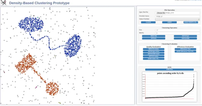
Figure 4.1 shows a snapshot of this test environment. The system has two main panels. The map panel on the left side is an interactive canvas in which the user can click and create data points. The tool bar on the right side is composed of input boxes, selection boxes, and buttons which are divided into different groups. Each group is used for a specific purpose, which will be discussed as below.
Figure 4.1: The Density-Based Clustering Test Environment 1http://stko.geog.ucsb.edu/adcn/
The “File Operation” tool group is used for point dataset manipulation. For simplic-ity, our environment defines a simple format for point datasets. Conceptually, a point dataset is a table containing the coordinates of points, their ground truth memberships, and the memberships produced during the experiments. The ground truth and experi-mental memberships are then compared to evaluate the cluster algorithms. The “Open Pts File” box is used for loading point datasets produced by other GIS. The data points can also be abstract points which represent objects, such as documents [7], in a feature space. The prototype takes the coordinates of points and maps out these points after rescaling their coordinates based on the size of the map panel. During the clustering process it uses Euclidean distance as the distance measure. The “PointSet Name” input box lets the user name the current point dataset displayed on the map panel. The “Select PointSet” selection box lists all the point datasets loaded into the system.
The “Clustering Operation” tool group is used to operate clustering tasks. The “Eps” and “MinPts” input boxes let users enter the clustering parameters for all clustering algorithms. The “DBSCAN”, “OPTICS”, “ADCN-Eps”, “ADCN-KNN” buttons are for running the algorithms. A user can click one of them to run the corresponding clustering algorithm on current point dataset based on the parameters (s)he entered earlier. As for the implementation of DBSCAN and OPTICS, we used a JavaScript clustering library from GitHub 2. This library has basic implementations of DBSCAN, OPTICS, K-MEANS, and some other clustering algorithms without any spatial indexes. Our ADCN-KNN and ADCN-Eps algorithms were implemented using the same data structures as used in the library. Such an implementation ensures that the evaluation result will reflect the differences of the algorithms rather than be affected by the specific data structures used in the implementations. Finally, we implemented an R-tree spatial index to accelerate the neighborhood search. We have used the R-tree JavaScript library
2
from GitHub3.
The “Clustering Evaluation” tool group is composed of “Quality Evaluation” and “Efficiency Evaluation” subgroups. As for the clustering quality evaluation, we imple-mented two metrics, Normalized mutual Information (NMI) and Rand Index, to quantify the goodness of the clustering results. The first four buttons in this subgroup will run the corresponding clustering algorithm on the current dataset based on all possible parameter combinations. They will compute two clustering evaluation indexes for each clustering result. The “SAVE Index As...” button will save these results to a text file.
Efficiency evaluation is another important part for comparing clustering algorithms. Density-based clustering algorithms are widely applied on large-scale data points. There-fore it is important to demonstrate the scalability of ADCN. The “Efficiency Evaluation” button will run these four clustering algorithms on datasets with different sizes. The “SAVE Efficiency Test As...” button can be further used to save the result into a text file.
Finally, the “KNN” tool group is used to draw the kth nearest neighbor plot (KNN plot) of the current dataset based on the MinPts parameter specified by the user. For each point, the KNN plot obtains the distance between the current point and its kth nearest point (hereK isMinPts). Then it ranks these kth nearest distance of each point in an ascending order. The KNN plot can be used for estimating the appropriate Eps
for the current point dataset given MinPts. More details this estimation can be found in the original DBSCAN paper [8].
Note that we provide the test environment to make our results reproducible and to offer a reusable implementation of ADCN, without implying that JavaScript would be the language of choice for future, large-scale applications of ADCN.
3
4.3
Evaluation of Clustering Quality
We use two clustering quality indices - the normalized mutual information (NMI) and the Rand Index - to measure the quality of clustering results of all algorithms. NMI originates from information theory and has been revised as an objective function for clustering ensembles [67]. NMI evaluates the accumulated mutual information shared by the clusters from different clustering algorithms. Let n be the number of points in a point datasets D. X = (X1, X2, ..., Xr) andY = (Y1, Y2, ..., Ys) are two clustering results from the same or different clustering algorithms. Note that noise points will be treated as their own cluster. Letn(hx) be the number of points in clusterXh and n
(y)
l the number of points in cluster Yl. Let n
(x,y)
h,l be the number of points in the intersect of cluster Xh and Yl. Then the normalized mutual information Φ(N M I)(X, Y) is defined in Equation 4.1 as the similarity between two clustering results X and Y:
Φ(N M I)(X, Y) = Pr h=1 Ps l=1n (x,y) h,l log n·n(h,lx,y) n(hx)·n(ly) q (Pr h=1n (x) h log n(hx) n )( Ps l=1n (y) l log n(ly) n ) (4.1)
Rand Index [58] is another objective function for clustering ensembles from a differ-ent perspective. It evaluates to which degree two clustering algorithms share the same relationships between points. Let abe the number of pairs of points inDthat are in the same clusters inX and in the same cluster in Y. b is the number of pairs of points inD that are in different clusters in X and Y. c is the number of pairs of points in D that are in the same clusters in X and in different cluster in Y. Finally, d is the number of pairs of points inD that are in different clusters inX and in the same cluster inY. The Rand Index Φ(Rand)(X, Y) is then defined as given by Equation 4.2:
Φ(Rand)(X, Y) = a+b
a+b+c+d (4.2)
For both NMI and Rand index, larger values indicate higher similarity between two clustering results. If a ground truth is available, both NMI and Rand can be used to compute the similarity between the result of an algorithms and the corresponding ground truth. This is called theextrinsic method [21].
We use the aforementioned 20 test cases to evaluate the clustering quality of DB-SCAN, ADCN-Eps, ADCN-KNN, and OPTICS. All of these four algorithms take the same parameters (Eps,M inP ts). As there are no established methods to determine the best overall parameter combination (we use KNN distance plots to estimate Eps) with re-spect to NMI and Rand Index, we stepwise tested every possible parameter combinations of Eps,M inP tscomputationally. An interactive 3D visualization of the NMI and Rand index results with changing Epsand M inP tsfor thespiral case with 0m buffer distance can be accessed online 4. Table 4.1 shows the maximum NMI and Rand Index results for the four algorithms over all test cases. Note that for each case, the best parameter combination with the maximum NMI does not necessarily yields the maximum Rand Index. However, among all of these 60 cases, there are 39, 35, 27, 39 cases for DBSCAN, ADCN-Eps, ADCN-KNN, OPTICS in which the best parameter combination for the maximum NMI is also the maximum Rand Index. For those cases where parameter com-binations of maximum NMI and maximum Rand do not match, their parameters tend to be close to each other because NMI and Rand values are changing continuously while Eps and M inP ts increase. This indicates that NMI and Rand Index have a medium to high similarity in terms of measuring the clustering quality.
As for the 60 test cases, ADCN-KNN has a higher maximum NMI/Rand Index than DBSCAN in 55 cases and has a higher maximum NMI/Rand Index than OPTICS in
55 cases; see also Figures 4.4 and 4.5. Even more, ADCN-KNN has a higher maximum NMI/Rand Index than ADCN-Eps in31cases; see Table 4.2. This indicates that ADCN-KNN gives the best clustering results among the tested algorithms. Our test cases do not only contain linear features but also cases that are typically used to evaluate algorithms such as DBSCAN, e.g., clusters of ellipsoid and rectangular shapes. In fact, these are the only cases were DBSCAN slightly out-competes ADCN-KNN, i.e., the maximum NMI/Rand Index of KNN and DBSCAN are comparable. Summing up, ADCN-KNN performs better than all other algorithms when dealing with anisotropic cases and equally well as DBSCAN for isotropic cases. In the following paragraphs, we will use ADCN-KNN and ADCN interchangeably.
Figure 4.2 and 4.3 show the point patterns as well as the best clustering results of all algorithms for the twelve synthesis cases and eight real-world cases without buffering, i.e., with the 0m buffer distance. By comparing best clustering results of these four algorithms, we can find some interesting patterns: 1) Connecting clusters along local directions: ADCN has a better ability to detect the local direction of spatial point patterns and connect the clusters along this direction; 2) Noise filtering: ADCN does better in filtering out noise points. A good example of connecting clusters along local directions is theellipseWidth case in Figure 4.2. As for the thinnest cluster in the bottom, the other 3 algorithms except ADCN-KNN extract multiple clusters from these points while ADCN-KNN is able to “connect” these clusters to a single one. Many cases show thenoise filtering advantage of ADCN. For example, thebridge case, themultiBridge case in Figure 4.2, and theBrooklyn Bridge case in Figure 4.3, reveal that ADCN is better at detecting and filtering out noise points along bridge-like features.
(a) (b)
Figure 4.2: Ground truth and best clustering result comparison for 12 synthesis cases.
4.4
Evaluation of Clustering Efficiency
This section discusses runtime differences of the four tested algorithms. Without a spatial index, the time complexity of all algorithms is O(n2). Eps-neighborhood queries consume the major part of the run time of density-based clustering algorithms [9], and, therefore, also of ADCN-KNN and ADCN-Eps in terms of Eps-ellipse-neighborhood queries. Hence, we implemented an R-tree to accelerate the neighborhood queries for all algorithms. This changes their time complexity to O(n log n).
In order to enable a comprehensible comparison of the run times of all algorithms on different sizes of point datasets, we performed a batch of performance tests. The polygons from the 20 cases shown above have been used to generated point datasets of different sizes ranging from 500 to 10000 in 500 step intervals. The ratio of noise points
to cluster points is set to 0.25. Eps,M inP tsare set to 15, 5 for all of these experiments. The average run times for the same size of point datasets is depicted in Figure 4.6.
Unsurprisingly, the runtime of all algorithms increases as the number of points in-creases. The runtime of ADCN-KNN is larger than that of DBSCAN and similar that of OPTICS. As the size of the point dataset increases, the ratio of the runtimes of ADCN-KNN to DBSCAN decrease from 2.80 to 1.29. The original OPTICS paper states a 1.6 runtime factor compared to DBSCAN. The used OPTICS library failed on datasets ex-ceeding 5500 points. We also fit the runtime data to the xlog(x) function. Figure 4.6 shows the fitted curves and functions of each clustering algorithm. We can see that allR2 of these functions are larger than 0.95 which means that the xlog(x) function well cap-tures the trends of the real runtime data of these clustering algorithms. For ADCN, our implementation tests for point-in-circle for the radius of the major axis before computing point-in-ellipse to significantly reduce the runtime. Further implementation optimiza-tions are possible but out of scope of this paper.
Table 4.1: Clustering quality comparisons
NMI Rand
Case Buffer DBSCAN ADCN-Eps ADCN-KNN OPTICS DBSCAN ADCN-Eps ADCN-KNN OPTICS
bridge 0m 0.937 0.957 0.957 0.937 0.985 0.991 0.992 0.985 5m 0.948 0.966 0.967 0.949 0.989 0.993 0.994 0.989 10m 0.938 0.973 0.968 0.944 0.988 0.995 0.995 0.989 circle 0m 0.864 0.865 0.912 0.864 0.955 0.964 0.978 0.955 5m 0.859 0.897 0.916 0.859 0.955 0.974 0.978 0.955 10m 0.864 0.911 0.923 0.864 0.960 0.979 0.982 0.960 circleNarrow 0m 0.914 0.951 0.958 0.914 0.974 0.988 0.991 0.974 5m 0.939 0.946 0.965 0.939 0.983 0.987 0.993 0.983 10m 0.923 0.962 0.962 0.923 0.976 0.991 0.992 0.976 circleRoad 0m 0.689 0.704 0.725 0.689 0.934 0.945 0.952 0.934 5m 0.737 0.758 0.779 0.737 0.950 0.963 0.962 0.951 10m 0.730 0.778 0.821 0.730 0.946 0.963 0.971 0.946 curve 0m 0.918 0.946 0.955 0.918 0.978 0.989 0.991 0.978 5m 0.924 0.947 0.956 0.924 0.980 0.990 0.992 0.980 10m 0.916 0.943 0.947 0.916 0.978 0.988 0.989 0.978 ellipse 0m 0.978 0.982 0.976 0.978 0.996 0.997 0.995 0.996 5m 0.979 0.982 0.980 0.979 0.996 0.997 0.996 0.996 10m 0.975 0.980 0.978 0.974 0.996 0.997 0.996 0.996 ellipseWidth 0m 0.917 0.935 0.935 0.917 0.985 0.989 0.988 0.985 5m 0.919 0.933 0.939 0.919 0.988 0.989 0.989 0.988 10m 0.931 0.938 0.941 0.931 0.990 0.991 0.991 0.989 multiBridge 0m 0.935 0.790 0.957 0.938 0.983 0.935 0.992 0.984 5m 0.958 0.883 0.977 0.958 0.992 0.968 0.996 0.992 10m 0.964 0.830 0.985 0.964 0.994 0.947 0.998 0.994 rectCurve 0m 0.886 0.893 0.907 0.886 0.963 0.969 0.973 0.963 5m 0.909 0.910 0.908 0.915 0.974 0.977 0.974 0.974 10m 0.921 0.923 0.911 0.922 0.975 0.977 0.977 0.975 spiral 0m 0.740 0.756 0.774 0.740 0.913 0.930 0.938 0.913 5m 0.776 0.812 0.809 0.776 0.927 0.946 0.948 0.927 10m 0.745 0.788 0.795 0.745 0.918 0.950 0.952 0.918 square 0m 0.745 0.751 0.794 0.745 0.934 0.920 0.944 0.934 5m 0.751 0.778 0.830 0.752 0.932 0.928 0.959 0.932 10m 0.744 0.716 0.801 0.743 0.935 0.893 0.944 0.935 star 0m 0.887 0.901 0.914 0.887 0.968 0.977 0.980 0.968 5m 0.903 0.899 0.916 0.900 0.974 0.977 0.982 0.974 10m 0.902 0.778 0.909 0.902 0.974 0.924 0.981 0.974 Brooklyn Bridge 0m 0.378 0.542 0.490 0.378 0.888 0.930 0.925 0.888 5m 0.442 0.604 0.579 0.440 0.900 0.943 0.941 0.900 10m 0.504 0.639 0.581 0.507 0.915 0.950 0.944 0.915 Brooktrail 0m 0.441 0.431 0.421 0.440 0.742 0.765 0.756 0.742 5m 0.476 0.512 0.489 0.475 0.750 0.825 0.800 0.750 10m 0.387 0.555 0.498 0.387 0.712 0.852 0.799 0.711 Eiffel Tower 0m 0.397 0.481 0.492 0.397 0.851 0.882 0.898 0.851 5m 0.459 0.566 0.571 0.459 0.868 0.906 0.921 0.868 10m 0.411 0.553 0.553 0.411 0.861 0.907 0.923 0.861 LAX 0m 0.557 0.607 0.593 0.557 0.867 0.898 0.905 0.867 5m 0.591 0.667 0.584 0.591 0.883 0.921 0.903 0.883 10m 0.485 0.590 0.637 0.479 0.857 0.903 0.925 0.857 Laicheng 0m 0.768 0.807 0.804 0.768 0.857 0.874 0.874 0.857 5m 0.761 0.815 0.808 0.761 0.856 0.878 0.905 0.856 10m 0.773 0.823 0.809 0.773 0.861 0.880 0.911 0.861 Skylawn 0m 0.618 0.822 0.733 0.618 0.871 0.956 0.927 0.871 5m 0.642 0.690 0.807 0.642 0.877 0.899 0.955 0.877 10m 0.729 0.703 0.822 0.729 0.927 0.905 0.957 0.927 Stelvio Pass 0m 0.640 0.715 0.717 0.656 0.945 0.962 0.963 0.946 5m 0.739 0.791 0.768 0.739 0.962 0.974 0.975 0.962 10m 0.686 0.798 0.766 0.686 0.953 0.975 0.978 0.953 Zhangjiajie 0m 0.760 0.832 0.799 0.760 0.964 0.978 0.976 0.964 5m 0.772 0.868 0.839 0.772 0.967 0.987 0.982 0.967 10m 0.835 0.911 0.873 0.835 0.978 0.991 0.990 0.978
Table 4.2: The number of cases with maximum NMI/Rand for each clustering algorithm # of cases Max NMI Max Rand
DBSCAN 1 0
ADCN-Eps 25 19
ADCN-KNN 33 41
Figure 4.4: Clustering quality comparisons: NMI Difference between 3 clustering methods and DBSCAN for each case. Synthetic cases are on the left, real-world cases on the right.
Figure 4.5: Clustering quality comparisons: Rand Difference between 3 clustering methods and DBSCAN for each case. Synthetic cases are on the left, real-world cases on the right.
Figure 4.6: Comparison of clustering efficiency with different dataset sizes; runtimes are given in millisecond (The used OPTICS library failed on datasets exceeding 5500 points)
Real World Application
In this chapter, we will discuss the application of ADCN for the computation of urban areas of interest (AOI) from user-generated geotagged photos collected by the Flickr plat-form. In Chapter 2 Section 2.1, we already mentioned multiple applications of density-based clustering algorithms. Since ADCN is part of the density-density-based clustering algo-rithm family, all the applications we discussed before can also use ADCN instead. Here, our focus is on how the results of ADCN differ from those of DBSCAN for common application examples in GIScience and computer science. Put differently, does the use of ADCN over DBSCAN produce significantly different results when it matters? We will focus on comparison here by relying on previous work as a ground truth for AOI is not available.
In previous work, Hu et al. [2] proposed a framework for extracting urban AOIs from geotagged photos. We will use the same workflow as Hu et al. did except we will apply four different algorithms, namely DBSCAN, OPTICS, ADCN-Eps, and ADCN-KNN, to the geotagged Flickr photos data to extract clusters. By comparing the extracted urban AOIs from different clustering algorithms, we can further understand the performance difference of these algorithms. We will briefly describe the workflow below. Readers