Linear Context-Free Rewriting Systems
Laura Kallmeyer
∗Heinrich-Heine-Universit¨at D ¨usseldorf
Wolfgang Maier
∗∗Heinrich-Heine-Universit¨at D ¨usseldorf
This paper presents the first efficient implementation of a weighted deductive CYK parser for Probabilistic Linear Context-Free Rewriting Systems (PLCFRSs). LCFRS, an extension of CFG, can describe discontinuities in a straightforward way and is therefore a natural candidate to be used for data-driven parsing. To speed up parsing, we use different context-summary estimates of parse items, some of them allowing for A∗parsing. We evaluate our parser with grammars extracted from the German NeGra treebank. Our experiments show that data-driven LCFRS parsing is feasible and yields output of competitive quality.
1. Introduction
Recently, the challenges that a rich morphology poses for data-driven parsing have received growing interest. A direct effect of morphological richness is, for instance, data sparseness on a lexical level (Candito and Seddah 2010). A rather indirect effect is that morphological richness often relaxes word order constraints. The principal intuition is that a rich morphology encodes information that otherwise has to be conveyed by a particular word order. If, for instance, the case of a nominal complement is not provided by morphology, it has to be provided by the position of the complement relative to other complements in the sentence. Example (1) provides an example of case marking and free word order in German. In turn, in free word order languages, word order can encode information structure (Hoffman 1995).
(1) a. der the
kleine little
Jungenom
boy
schickt sends
seiner his
Schwesterdat
sister
den the
Briefacc
letter
b. Other possible word orders:
(i) der kleine Jungenomschickt den Briefaccseiner Schwesterdat
(ii) seiner Schwesterdatschickt der kleine Jungenomden Briefacc
(iii) den Briefaccschickt der kleine Jungenomseiner Schwesterdat
∗Institut f ¨ur Sprache und Information, Universit¨atsstr. 1, D-40225 D ¨usseldorf, Germany. E-mail:[email protected].
∗∗Institut f ¨ur Sprache und Information, Universit¨atsstr. 1, D-40225 D ¨usseldorf, Germany. E-mail:[email protected].
It is assumed that this relation between a rich morphology and free word order does not hold in both directions. Although it is generally the case that languages with a rich morphology exhibit a high degree of freedom in word order, languages with a free word order do not necessarily have a rich morphology. Two examples for languages with a very free word order are Turkish and Bulgarian. The former has a very rich and the latter a sparse morphology. See M ¨uller (2002) for a survey of the linguistics literature on this discussion.
With a rather free word order, constituents and single parts of them can be displaced freely within the sentence. German, for instance, has a rich inflectional system and allows for a free word order, as we have already seen in Example (1): Arguments can be scrambled, and topicalizations and extrapositions underlie few restrictions. Conse-quently, discontinuous constituents occur frequently. This is challenging for syntactic description in general (Uszkoreit 1986; Becker, Joshi, and Rambow 1991; Bunt 1996; M ¨uller 2004), and for treebank annotation in particular (Skut et al. 1997).
In this paper, we address the problem of data-driven parsing of discontinuous constit-uents on the basis of German. In this section, we inspect the type of data we have to deal with, and we describe the way such data are annotated in treebanks. We briefly discuss different parsing strategies for the data in question and motivate our own approach.
1.1 Discontinuous Constituents
Consider the sentences in Example (2) as examples for discontinuous constituents (taken from the German NeGra [Skut et al. 1997] and TIGER [Brants et al. 2002] tree-banks). Example (2a) shows several instances of discontinuous VPs and Example (2b) shows a discontinuous NP. The relevant constituent is printed in italics.
(2) a. Fronting:
(i) Dar ¨uber Thereof muss must nachgedacht thought werden. be (NeGra)
“One must think of that”
(ii) Ohne internationalen Schaden Without international damage
k ¨onne could sich itself Bonn Bonn
von dem Denkmal from the monument
nicht not
distanzieren,
distance
... (TIGER)
“Bonn could not distance itself from the monument without international damage.”
(iii) Auch
Also
w ¨urden would
durch die Regelung through the regulation
nur only “st¨andig “constantly neue new Altf¨alle old cases
entstehen”. (TIGER)
emerge”
“Apart from that, the regulation would only constantly produce new old cases.”
b. Extraposed relative clauses:
(i) . . . ob . . . whether
auf on deren their Gel¨ande terrain der the
Typ von Abstellanlage type of parking facility
gebaut built werden get k ¨onne, could, der ... which . . .
(NeGra)
Examples of other such languages are Bulgarian and Korean. Both show discontin-uous constituents as well. Example (3a) is a Bulgarian example of a PP extracted out of an NP, taken from the BulTreebank (Osenova and Simov 2004), and Example (3b) is an example of fronting in Korean, taken from the Penn Korean Treebank (Han, Han, and Ko 2001).
(3) a. Na kyshtata Of house-DET
toi he
popravi repaired
pokriva.
roof.
“It is the roof of thehousehe repairs.”
b. Gwon.han- ˘ul Authority-OBJ
nu.ga who
ka.ji.go has
iss.ji? not?
“Who has no authority?”
Discontinuous constituents are by no means limited to languages with freedom in word order. They also occur in languages with a rather fixed word order such as English, resulting from, for instance, long-distance movements. Examples (4a) and (4b) are examples from the Penn Treebank for long extractions resulting in discontin-uous S categories and for discontindiscontin-uous NPs arising from extraposed relative clauses, respectively (Marcus et al. 1994).
(4) a. Long Extraction in English:
(i) Those chains include Bloomingdale’s,whichCampeau recently saidit will sell.
(ii) Whatshould Ido.
b. Extraposed nominal modifiers (relative clauses and PPs) in English:
(i) They sowa row of male-fertile plantsnearby,which then pollinate the male-sterile plants.
(ii) Pricesfell marginallyfor fuel and electricity.
1.2 Treebank Annotation and Data-Driven Parsing
Most constituency treebanks rely on an annotation backbone based on Context-Free Grammar (CFG). Discontinuities cannot be modeled with CFG, because they require a larger domain of locality than the one offered by CFG. Therefore, the annotation back-bone based on CFG is generally augmented with a separate mechanism that accounts for the non-local dependencies. In the Penn Treebank (PTB), for example, trace nodes and co-indexation markers are used in order to establish additional implicit edges in the tree beyond the overt phrase structure. In T ¨uBa-D/Z (Telljohann et al. 2012), a German Treebank, non-local dependencies are expressed via an annotation of topological fields (H ¨ohle 1986) and special edge labels. In contrast, some other treebanks, among them NeGra and TIGER, give up the annotation backbone based on CFG and allow annota-tion with crossing branches (Skut et al. 1997). In such an annotaannota-tion, non-local depen-dencies can be expressed directly by grouping all dependent elements under a single node. Note that both crossing branches and traces annotate long-distance dependencies in a linguistically meaningful way. A difference is, however, that crossing branches are less theory-dependent because they do not make any assumptions about the base positions of “moved” elements.
Figure 1
A discontinuous constituent. Original NeGra annotation (left) and a T ¨uBa-D/Z-style annotation (right).
What WP
should MD
I PRP
do VB
*T*
-NONE-? .
WHNP NP NP
VP SBJ
SQ SBARQ
*T*
What WP
should MD
I PRP
do VB
? .
WHNP NP
VP
SBJ
SQ SBARQ
Figure 2
A discontinuous wh-movement. Original PTB annotation (left) and NeGra-style annotation (right).
annotation of the same sentence in the style of the T ¨uBa-D/Z treebank (right). Figure 2 shows the PTB annotation of Example (4a-ii) (on the left, note that the directed edge from the trace to the WHNP element visualizes the co-indexation) together with a NeGra-style annotation of the same sentence (right).
In the past, data-driven parsing has largely been dominated by Probabilistic Context-Free Grammar (PCFG). In order to extract a PCFG from a treebank, the trees need to be interpretable as CFG derivations. Consequently, most work has excluded non-local dependencies; either (in PTB-like treebanks) by discarding labeling conven-tions such as the co-indexation of the trace nodes in the PTB, or (in NeGra/TIGER-like treebanks) by applying tree transformations, which resolve the crossing branches (e.g., K ¨ubler 2005; Boyd 2007). Especially for the latter treebanks, such a transformation is problematic, because it generally is non-reversible and implies information loss.
Discontinuities are no minor phenomenon: Approximately 25% of all sentences in NeGra and TIGER have crossing branches (Maier and Lichte 2011). In the Penn Treebank, this holds for approximately 20% of all sentences (Evang and Kallmeyer 2011). This shows that it is important to properly treat such structures.
1.3 Extending the Domain of Locality
[image:4.486.50.310.207.327.2]CFG:
A
γ
LCFRS: •
A
• •
[image:5.486.53.251.61.148.2]γ1 γ2 γ3
Figure 3
Different domains of locality.
mechanism (Chiang 2003). The second class, to which we contribute in this paper, consists of approaches that aim at producing trees which contain non-local information. Some methods realize the reconstruction of non-local information in a post- or pre-processing step to PCFG parsing (Johnson 2002; Dienes 2003; Levy and Manning 2004; Cai, Chiang, and Goldberg 2011). Other work uses formalisms that accommodate the direct encoding of non-local information (Plaehn 2004; Levy 2005). We pursue the latter approach.
Our work is motivated by the following recent developments. Linear Context-Free Rewriting Systems (LCFRSs) (Vijay-Shanker, Weir, and Joshi 1987) have been estab-lished as a candidate for modeling both discontinuous constituents and non-projective dependency trees as they occur in treebanks (Maier and Søgaard 2008; Kuhlmann and Satta 2009; Maier and Lichte 2011). LCFRSs are a natural extension of CFGs where the non-terminals can span tuples of possibly non-adjacent strings (see Figure 3). Be-cause LCFRSs allow for binarization and CYK chart parsing in a way similar to CFGs, PCFG techniques, such as best-first parsing (Caraballo and Charniak 1998), weighted deductive parsing (Nederhof 2003), and A∗ parsing (Klein and Manning 2003a) can be transferred to LCFRS. Finally, as mentioned before, languages such as German have recently attracted the interest of the parsing community (K ¨ubler and Penn 2008; Seddah, K ¨ubler, and Tsarfaty 2010).
We bring together these developments by presenting a parser for Probabilistic LCFRS (PLCFRS), continuing the promising work of Levy (2005). Our parser pro-duces trees with crossing branches and thereby accounts for syntactic long-distance dependencies while not making any additional assumptions concerning the position of hypothetical traces. We have implemented a CYK parser and we present several methods for context summary estimation of parse items. The estimates either act as figures-of-merit in a best-first parsing context or as estimates for A∗parsing. A test on a real-world-sized data set shows that our parser achieves competitive results. To our knowledge, our parser is the first for the entire class of PLCFRS that has successfully been used for data-driven parsing.1
The paper is structured as follows. Section 2 introduces probabilistic LCFRS. Sec-tions 3 and 4 present the binarization algorithm, the parser, and the outside estimates which we use to speed up parsing. In Section 5 we explain how to extract an LCFRS from a treebank and we present grammar refinement methods for these specific treebank grammars. Finally, Section 6 presents evaluation results and Section 7 compares our work to other approaches.
2. Probabilistic Linear Context-Free Rewriting Systems
2.1 Definition of PLCFRS
LCFRS (Vijay-Shanker, Weir, and Joshi 1987) is an extension of CFG in which a non-terminal can span not only a single string but a tuple of strings of sizek≥1.kis thereby called its fan-out. We will notate LCFRS with the syntax ofSimple Range Concate-nation Grammars(SRCG) (Boullier 1998b), a formalism that is equivalent to LCFRS. A third formalism that is equivalent to LCFRS is Multiple Context-Free Grammar
(MCFG) (Seki et al. 1991).
Definition 1 (LCFRS)
ALinear Context-Free Rewriting System(LCFRS) is a tupleN,T,V,P,Swhere
a) Nis a finite set of non-terminals with a functiondim:N→Nthat determines thefan-outof eachA∈N;
b) TandVare disjoint finite sets of terminals and variables; c) S∈Nis the start symbol withdim(S)=1;
d) Pis a finite set of rules
A(α1,. . .,αdim(A))→A1(X1(1),. . .,X (1)
dim(A1))· · ·Am(X
(m) 1 ,. . .,X
(m)
dim(Am))
form≥0 whereA,A1,. . .,Am ∈N,Xj(i)∈Vfor 1≤i≤m, 1≤j≤dim(Ai)
andαi∈(T∪V)∗for 1≤i≤dim(A). For allr∈P, it holds that every
variableXoccurring inroccurs exactly once in the left-hand side and exactly once in the right-hand side ofr.
A rewriting rule describes how the yield of the left-hand side non-terminal can be computed from the yields of the right-hand side non-terminals. The rulesA(ab,cd)→ε
and A(aXb,cYd)→A(X,Y) from Figure 4 for instance specify that (1)ab,cdis in the yield ofAand (2) one can compute a new tuple in the yield ofAfrom an already existing one by wrappingaandbaround the first component andcand daround the second. A CFG ruleA→BCwould be writtenA(XY)→B(X)C(Y) as an LCFRS rule.
Definition 2 (Yield, language)
LetG=N,T,V,P,Sbe an LCFRS.
1. For everyA∈N, we define theyieldofA,yield(A) as follows: a) For every ruleA(α)→ε,α ∈yield(A);
A(ab,cd) → ε A(aXb,cYd) → A(X,Y)
S(XY) → A(X,Y)
Figure 4
b) For every ruleA(α1,. . .,αdim(A))→A1(X(1)1 ,. . .,X (1)
dim(A1))· · ·
Am(X(1m),. . .,X (m)
dim(Am)) and for allτi∈yield(Ai) (1≤i≤m):
f(α1),. . .,f(αdim(A)) ∈yield(A) wheref is defined as follows: (i) f(t)=tfor allt∈T,
(ii) f(X(ji))=τi(j) for all 1≤i≤m, 1≤j≤dim(Ai) and
(iii) f(xy)=f(x)f(y) for allx,y∈(T∪V)+.
We callf thecomposition functionof the rule.
c) Nothing else is inyield(A).
2. The language ofGis thenL(G)={w| w ∈yield(S)}.
As an example, consider again the LCFRS in Figure 4. The last rule tells us that, given a pair in the yield ofA, we can obtain an element in the yield ofSby concate-nating the two components. Consequently, thelanguagegenerated by this grammar is {anbncndn|n≥1}.
The terms of grammar fan-out and rank and the properties of monotonicity and
ε-freeness will be referred to later and are therefore introduced in the following defini-tion. They are taken from the LCFRS/MCFG terminology; the SRCG term for fan-out is
arityand the property of being monotone is calledorderedin the context of SRCG.
Definition 3
LetG=N,T,V,P,Sbe an LCFRS.
1. Thefan-outofGis the maximal fan-out of all non-terminals inG. 2. Furthermore, the right-hand side length of a rewriting ruler∈Pis called
therankofrand the maximal rank of all rules inPis called therankofG. 3. Gismonotoneif for everyr∈Pand every right-hand side non-terminalA
inrand each pairX1,X2of arguments ofAin the right-hand side ofr,X1
precedesX2in the right-hand side iffX1precedesX2in the left-hand side.
4. A ruler∈Pis called anε-rule if one of the left-hand side components ofr
isε.
Gisε-freeif it either contains noε-rules or there is exactly oneε-rule
S(ε)→εandSdoes not appear in any of the right-hand sides of the rules in the grammar.
For every LCFRS there exists an equivalent LCFRS that is ε-free (Seki et al. 1991; Boullier 1998a) and monotone (Michaelis 2001; Kracht 2003; Kallmeyer 2010).
The definition of a probabilistic LCFRS is a straightforward extension of the defini-tion of PCFG and thus it follows (Levy 2005; Kato, Seki, and Kasami 2006) that:
Definition 4 (PLCFRS)
Aprobabilistic LCFRS(PLCFRS) is a tupleN,T,V,P,S,psuch thatN,T,V,P,Sis an LCFRS andp:P→[0..1] a function such that for allA∈N:
PLCFRS with non-terminals{S,A,B}, terminals{a}and start symbolS: 0.2 :S(X)→A(X) 0.8 :S(XY)→B(X,Y)
0.7 :A(aX)→A(X) 0.3 :A(a)→ε
0.8 :B(aX,aY)→B(X,Y) 0.2 :B(a,a)→ε
Figure 5 Sample PLCFRS.
As an example, consider the PLCFRS in Figure 5. This grammar simply generates
a+. Words with an even number of as and nested dependencies are more probable than words with a right-linear dependency structure. For instance, the wordaareceives the two analyses in Figure 6. The analysis (a) displaying nested dependencies has probability 0.16 and (b) (right-linear dependencies) has probability 0.042.
3. Parsing PLCFRS
3.1 Binarization
Similarly to the transformation of a CFG into Chomsky normal form, an LCFRS can be binarized, resulting in an LCFRS of rank 2. As in the CFG case, in the transformation, we introduce a non-terminal for each right-hand side longer than 2 and split the rule into two rules, using this new intermediate non-terminal. This is repeated until all right-hand sides are of length 2. The transformation algorithm is inspired by G ´omez-Rodr´ıguez et al. (2009) and it is also specified in Kallmeyer (2010).
3.1.1 General Binarization. In order to give the algorithm for this transformation, we need the notion of areductionof a vectorα∈[(T∪V)∗]iby a vectorx∈Vjwhere all variables inxoccur inα. A reduction is, roughly, obtained by keeping all variables inα
that are not inx. This is defined as follows:
Definition 5 (Reduction)
LetN,T,V,P,Sbe an LCFRS,α ∈[(T∪V)∗]iandx∈Vjfor somei,j∈IN.
Letw=α1$. . .$αibe the string obtained from concatenating the components ofα,
separated by a new symbol $∈/(V∪T).
Letwbe the image ofwunder a homomorphismhdefined as follows:h(a)=$ for alla∈T,h(X)=$ for allX∈ {x1,. . .xj}andh(y)=yin all other cases.
Let y1,. . .ym∈V+ such that w∈$∗y1$+y2$+. . .$+ym$∗. Then the vector
y1,. . .ymis thereductionofαbyx.
For instance,aX1,X2,bX3reduced withX2 yieldsX1,X3and aX1X2bX3
re-duced withX2yieldsX1,X3as well.
S
B
a a
(a)
S
A
a A
[image:8.486.50.178.561.634.2]a (b)
Figure 6
forall rulesr=A(α)→A0(α0). . .Am(αm) inPwithm>1do
removerfromP R:=∅
pick new non-terminalsC1,. . .,Cm−1
add the ruleA(α) →A0(α0)C1(γ1) toRwhereγ1is obtained by reducingαwithα0
foralli, 1≤i≤m−2do
add the ruleCi(γi)→Ai(αi)Ci+1(γi+1) toRwhereγi+1is obtained by reducingγiwithαi
end for
add the ruleCm−1(γm−2)→Am−1(αm−1)Am(αm) toR
forevery ruler∈Rdo
replace right-hand side arguments of length>1 with new variables (in both sides) and add the result toP
end for end for Figure 7
Algorithm for binarizing an LCFRS.
The binarization algorithm is given in Figure 7. As already mentioned, it proceeds like the CFG binarization algorithm in the sense that for right-hand sides longer than 2, we introduce a new non-terminal that covers the right-hand side without the first element. Figure 8 shows an example. In this example, there is only one rule with a right-hand side longer than 2. In a first step, we introduce the new non-terminals and rules that binarize the right-hand side. This leads to the setR. In a second step, before adding the rules fromRto the grammar, whenever a right-hand side argument contains several variables, these are collapsed into a single new variable.
The equivalence of the original LCFRS and the binarized grammar is rather straight-forward. Note, however, that the fan-out of the LCFRS can increase.
The binarization depicted in Figure 7 is deterministic in the sense that for every rule that needs to be binarized, we choose unique new non-terminals. Later, in Section 5.3.1, we will introduce additional factorization into the grammar rules that reduces the set of new non-terminals.
3.1.2 Minimizing Fan-Out and Number of Variables.In LCFRS, in contrast to CFG, the order of the right-hand side elements of a rule does not matter for the result of a derivation.
Original LCFRS:
S(XYZUVW)→A(X,U)B(Y,V)C(Z,W) A(aX,aY)→A(X,Y) A(a,a)→ε B(bX,bY)→B(X,Y) B(b,b)→ε C(cX,cY)→C(X,Y) C(c,c)→ε
Rule with right-hand side of length>2:S(XYZUVW)→A(X,U)B(Y,V)C(Z,W) For this rule, we obtain
R={S(XYZUVW)→A(X,U)C1(YZ,VW),C1(YZ,VW)→B(Y,V)C(Z,W)}
Equivalent binarized LCFRS: S(XPUQ)→A(X,U)C1(P,Q)
C1(YZ,VW)→B(Y,V)C(Z,W)
A(aX,aY)→A(X,Y) A(a,a)→ε B(bX,bY)→B(X,Y) B(b,b)→ε C(cX,cY)→C(X,Y) C(c,c)→ε Figure 8
Therefore, we can reorder the right-hand side of a rule before binarizing it. In the following, we present a binarization order that yields a minimal fan-out and a minimal variable number per production and binarization step. The algorithm is inspired by G ´omez-Rodr´ıguez et al. (2009) and has first been published in this version in Kallmeyer (2010). We assume that we are only considering partitions of right-hand sides where one of the sets contains only a single non-terminal.
For a given rulec=A0(x0)→A1(x1). . .Ak(xk), we define thecharacteristic string s(c,Ai) of theAi-reduction ofcas follows: Concatenate the elements ofx0, separated with
new additional symbols $ while replacing every component fromxiwith a $. We then
define the arity of the characteristic string,dim(s(c,Ai)), as the number of maximal
sub-stringsx∈V+ins(A
i). Take, for example, a rulec=VP(X,YZU)→VP(X,Z)V(Y)N(U).
Thens(c,VP)=$$Y$U,s(c,V)=X$$ZU.
Figure 9 shows how in a first step, for a given rulerwith right-hand side length>2, we determine the optimal candidate for binarization based on the characteristic string
s(r,B) of some right-hand side non-terminal Band on the fan-out of B: On all right-hand side predicatesBwe check for the maximal fan-out (given bydim(s(r,B))) and the number of variables (dim(s(r,B))+dim(B)) we would obtain when binarizing with this predicate. This check provides the optimal candidate. In a second step we then perform the same binarization as before, except that we use the optimal candidate now instead of the first element of the right-hand side.
3.2 The Parser
We can assume without loss of generality that our grammars areε-free and monotone (the treebank grammars with which we are concerned all have these properties) and that they contain only binary and unary rules. Furthermore, we assume POS tagging to be done before parsing. POS tags are non-terminals of fan-out 1. Finally, according to our grammar extraction algorithm (see Section 5.1), a separation between two components always means that there is actually a non-empty gap in between them. Consequently, two different components in a right-hand side can never be adjacent in the same component of the left-hand side. The rules are then either of the formA(a)→εwithAa POS tag anda∈Tor of the formA(x)→B(x) orA(α)→B(x)C(y) whereα ∈(V+)dim(A),
x∈Vdim(B),y∈Vdim(C), that is, only the rules for POS tags contain terminals in their left-hand sides.
cand=0
fan-out= number of variables inr vars= number of variables inr for alli=0tomdo
cand-fan-out=dim(s(r,Ai));
ifcand-fan-out<fan-outanddim(Ai)<fan-outthen
fan-out=max({cand-fan-out,dim(Ai)});
vars=cand-fan-out+dim(Ai);
cand=i;
else ifcand-fan-out≤fan-out,dim(Ai)≤fan-outandcand-fan-out+dim(Ai)<varsthen
fan-out=max({cand-fan-out,dim(Ai)});
vars=cand-fan-out+dim(Ai);
cand=i end if end for
Figure 9
During parsing we have to link the terminals and variables in our LCFRS rules to portions of the input string. For this purpose we need the notions of ranges, range vectors, and rule instantiations. A range is a pair of indices that characterizes the span of a component within the input. A range vector characterizes a tuple in the yield of a non-terminal. A rule instantiation specifies the computation of an element from the left-hand side yield from elements in the yields of the right-left-hand side non-terminals based on the corresponding range vectors.
Definition 6 (Range)
Letw∈T∗withw=w1. . .wnwherewi∈Tfor 1≤i≤n.
1. Pos(w) :={0,. . .,n}.
2. We call a pairl,r ∈Pos(w)×Pos(w) withl≤rarangeinw. Itsyield
l,r(w) is the substringwl+1. . .wr.
3. For two rangesρ1=l1,r1,ρ2 =l2,r2, ifr1 =l2, then the concatenation
ofρ1andρ2isρ1·ρ2 =l1,r2; otherwiseρ1·ρ2is undefined.
4. Aρ∈(Pos(w)×Pos(w))kis ak-dimensionalrange vectorforwiff
ρ=l1,r1,. . .,lk,rkwhereli,riis a range inwfor 1≤i≤k.
We now define instantiations of rules with respect to a given input string. This definition follows the definition ofclause instantiationsfrom Boullier (2000). An in-stantiated rule is a rule in which variables are consistently replaced by ranges. Because we need this definition only for parsing our specific grammars, we restrict ourselves to
ε-free rules containing only variables.
Definition 7 (Rule instantiation)
Let G=(N,T,V,P,S) be an ε-free monotone LCFRS. For a given ruler=A(α)→
A1(x1)· · ·Am(xm)∈P(0<m) that does not contain any terminals,
1. aninstantiationwith respect to a stringw=t1. . .tnconsists of a function f :V→ {i,j |1≤i≤j≤ |w|}such that for allx,yadjacent in one of the elements ofα,f(x)·f(y) must be defined; we then definef(xy)=f(x)·f(y), 2. iff is an instantiation ofr, thenA(f(α))→A1(f(x1))· · ·Am(f(xm)) is an
instantiated rulewheref(x1,. . .,xk)=f(x1),. . .,f(xk).
We use a probabilistic version of the CYK parser from Seki et al. (1991). The algo-rithm is formulated using the framework of parsing as deduction (Pereira and Warren 1983; Shieber, Schabes, and Pereira 1995; Sikkel 1997), extended with weights (Nederhof 2003). In this framework, a set of weighted items representing partial parsing results is characterized via a set of deduction rules, and certain items (the goal items) represent successful parses.
During parsing, we have to match components in the rules we use with portions of the input string. For a given inputw, our items have the form [A,ρ] whereA∈Nandρ
is a range vector that characterizes the span ofA. Each item has a weightinthat encodes the Viterbi inside score of its best parse tree. More precisely, we use the log probability log(p) wherepis the probability.
Scan: 0 : [A,i,i+1] Ais the POS tag ofwi+1
Unary: in: [B,ρ]
in+log(p) : [A,ρ] p:A(α)→B(α)∈P Binary: ininB: [B,ρB],inC: [C,ρC]
B+inC+log(p) : [A,ρA]
p:A(ρA)→B(ρB)C(ρC)
is an instantiated rule
Goal: [S,0,n] Figure 10
Weighted CYK deduction system.
second rule, unary, is applied whenever we have found the right-hand side of an instantiation of a unary rule. In our grammar, terminals only occur in rules with POS tags and the grammar is ordered andε-free. Therefore, the components of the yield of the right-hand side non-terminal and of the left-hand side terminals are the same. The rulebinaryapplies an instantiated rule of rank 2. If we already have the two elements of the right-hand side, we can infer the left-hand side element. In both cases, unary
andbinary, the probabilitypof the new rule is multiplied with the probabilities of the antecedent items (which amounts to summing up the antecedent weights andlog(p)).
We perform weighted deductive parsing, based on the deduction system from Figure 10. We use a chart C and an agenda A, both initially empty, and we proceed as in Figure 11. Because for all our deduction rules, the weight functionsf that compute the weight of a consequent item from the weights of the antecedent items are monotone non-increasing in each variable, the algorithm will always find the best parse without the need of exhaustive parsing. All new items that we deduce involve at least one of the agenda items as an antecedent item. Therefore, whenever an item is the best in the agenda, we can be sure that we will never find an item with a better (i.e., higher) weight. Consequently, we can safely store this item in the chart and, if it is a goal item, we have found the best parse.
As an example consider the development of the agenda and the chart in Figure 12 when parsing aa with the PLCFRS from Figure 5, transformed into a PLCFRS with pre-terminals and binarization (i.e., with a POS tag Ta and a new binarization
non-terminalB). The new PLCFRS is given in Figure 13.
In this example, we find a first analysis for the input (a goal item) when combining an Awith span0, 2into anS. This Shas however a rather low probability and is therefore not on top of the agenda. Later, when finding the better analysis, the weight
add SCANresults toA
whileA=∅
remove best itemx:IfromA addx:ItoC
ifIgoal item
thenstop and output true else
for ally:Ideduced fromx:Iand items inC: ifthere is nozwithz:I∈ C ∪ A
thenaddy:ItoA else ifz:I∈ Afor somez
thenupdate weight ofIinAtomax(y,z) Figure 11
chart agenda
0 : [Ta,0, 1], 0 : [Ta,1, 2]
0 : [Ta,0, 1] 0 : [Ta,1, 2],−0.5 : [A,0, 1]
0 : [Ta,0, 1], 0 : [Ta,1, 2] −0.5 : [A,0, 1],−0.5 : [A,1, 2],
−0.7 : [B,0, 1,1, 2]
0 : [Ta,0, 1], 0 : [Ta,1, 2], −0.5 : [A,1, 2],−0.7 : [B,0, 1,1, 2],
−0.5 : [A,0, 1] −1.2 : [S,0, 1]
0 : [Ta,0, 1], 0 : [Ta,1, 2], −0.65 : [A,0, 2],−0.7 : [B,0, 1,1, 2],
0.5 : [A,0, 1],−0.5 : [A,1, 2] −1.2 : [S,0, 1],−1.2 : [S,1, 2] 0 : [Ta,0, 1], 0 : [Ta,1, 2], −0.7 : [B,0, 1,1, 2],−1.2 : [S,0, 1],
−0.5 : [A,0, 1],−0.5 : [A,1, 2], −1.2 : [S,1, 2],−1.35 : [S,0, 2]
−0.65 : [A,0, 2]
0 : [Ta,0, 1], 0 : [Ta,1, 2], −0.8 : [S,0, 2],−1.2 : [S,0, 1],
−0.5 : [A,0, 1],−0.5 : [A,1, 2], −1.2 : [S,1, 2]
[image:13.486.52.393.62.217.2]−0.65 : [A,0, 2],−0.7 : [B,0, 1,1, 2] Figure 12
Parsing ofaawith the grammar from Figure 5.
PLCFRS with non-terminals{S,A,B,B,Ta}, terminals{a}and start symbolS:
0.2 :S(X)→A(X) 0.8 :S(XY)→B(X,Y) 0.7 :A(XY)→Ta(X)A(Y) 0.3 :A(X)→Ta(X)
0.8 :B(ZX,Y)→Ta(Z)B(X,Y) 1 :B(X,UY)→B(X,Y)Ta(U)
0.2 :B(X,Y)→Ta(X)Ta(Y) 1 :Ta(a)→ε
Figure 13
Sample binarized PLCFRS (with pre-terminalTa).
of theSitem in the agenda is updated and then the goal item is the top agenda item and therefore parsing has been successful.
Note that, so far, we have only presented the recognizer. In order to extend it to a parser, we do the following: Whenever we generate a new item, we store it not only with its weight but also with backpointers to its antecedent items. Furthermore, whenever we update the weight of an item in the agenda, we also update the backpointers. In order to read off the best parse tree, we have to start from the goal item and follow the backpointers.
4. Outside Estimates
So far, the weights we use give us only the Viterbi inside score of an item. In order to speed up parsing, we add the estimate of the costs for completing the item into a goal item to its weight—that is, to the weight of each item in the agenda, we add an estimate of its Viterbi outside score2(i.e., the logarithm of the estimate). We usecontext
summary estimates. A context summary is an equivalence class of items for which we can compute the actual outside scores. Those scores are then used as estimates. The challenge is to choose the estimate general enough to be efficiently computable and specific enough to be helpful for discriminating items in the agenda.
Admissibility and monotonicity are two important conditions on estimates. All our outside estimates are admissible (Klein and Manning 2003a), which means that they never underestimate the actual outside score of an item. In other words, they are too optimistic about the costs of completing the item into anSitem spanning the entire input. For the full SX estimate described in Section 4.1 and the SX estimate with span and sentence length in Section 4.4, the monotonicity is guaranteed and we can do true A∗parsing as described by Klein and Manning. Monotonicity means that for each antecedent item of a rule it holds that its weight is greater than or equal to the weight of the consequent item. The estimates from Sections 4.2 and 4.3 are not monotonic. This means that it can happen that we deduce an itemI2from an itemI1where the weight of
I2 is greater than the weight ofI1. The parser can therefore end up in a local maximum
that is not the global maximum we are searching for. In other words, those estimates are onlyfigures of merit(FOM).
All outside estimates are computed off-line for a certain maximal sentence length
lenmax.
4.1 Full SX Estimate
The full SX estimate is a PLCFRS adaption of theSX estimate of Klein and Manning (2003a) (hence the name). For a given sentence lengthn, the estimate gives the maximal probability of completing a categoryXwith a spanρinto anSwith span0,n.
For its computation, we need an estimate of the inside score of a categoryCwith a spanρ, regardless of the actual terminals in our input. This inside estimate is computed as shown in Figure 14. Here, we do not need to consider the number of terminals outside the span ofC(to the left or right or in the gaps), because they are not relevant for the inside score. Therefore the items have the form [A,l1,. . .,ldim(A)], whereAis a
non-terminal andligives the length of itsith component. It holds that
Σ1≤i≤dim(A)li≤lenmax−dim(A)+1
because our grammar extraction algorithm ensures that the different components in the yield of a non-terminal are never adjacent. There is always at least one terminal in between two different components that does not belong to the yield of the non-terminal. The first rule in Figure 14 tells us that POS tags always have a single component of length 1; therefore this case has probability 1 (weight 0). The rulesunaryandbinary
are roughly like the ones in the CYK parser, except that they combine items with length information. The rule unaryfor instance tells us that if the log of the probability of building [B,l] is greater or equal toin and if there is a rule that allows to deduce an
POS tags: 0 : [A,1] Aa POS tag Unary: in: [B,l]
in+log(p) : [A,l] p:A(α)→B(α)∈P
Binary: inB: [B,lB],inC: [C,lC] inB+inC+log(p) : [A,lA]
wherep:A(αA)→B(αB)C(αC)∈Pand the following holds: we defineB(i) as
{1≤j≤dim(B)|αB(j) occurs inαA(i)}andC(i) as{1≤j≤dim(C)|αC(j) occurs inαA(i)}.
Then for alli, 1≤i≤dim(A):lA(i)= Σj∈B(i)lB(j)+ Σj∈C(i)lC(j).
Figure 14
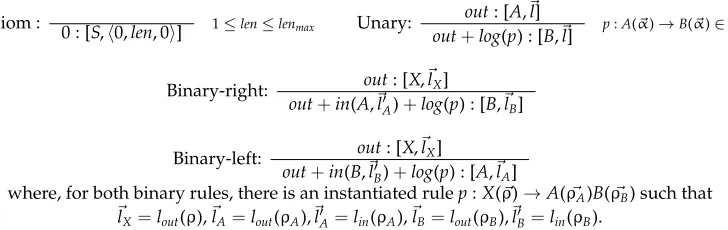
Axiom :
0 : [S,0,len, 0] 1≤len≤lenmax Unary: out: [A,
l]
out+log(p) : [B,l] p:A(α)→B(α)∈P
Binary-right: out: [X,lX]
out+in(A,lA)+log(p) : [B,lB]
Binary-left: out: [X,lX]
out+in(B,lB)+log(p) : [A,lA]
where, for both binary rules, there is an instantiated rulep:X(ρ)→A(ρA)B(ρB) such that
lX=lout(ρ),lA=lout(ρA),l
[image:15.486.65.429.64.179.2]A=lin(ρA),lB=lout(ρB),lB=lin(ρB).
Figure 15
Full SX estimate first version (top–down).
Aitem from [B,l] with probabilityp, then the log of the probability of [A,l] is greater or equal toin+log(p). For each item, we record its maximal weight (i.e., its maximal probability). The rulebinaryis slightly more complicated because we have to compute the length vector of the left-hand side of the rule from the right-hand side length vectors. A straightforward extension of the CFG algorithm from Klein and Manning (2003a) for computing the SX estimate is given in Figure 15. Here, the items have the form [A,l] where the vectorltells us about the lengths of the string to the left of the first component, the first component, the string in between the first and second component, and so on.
The algorithm proceeds top–down. The outside estimate of completing anSwith component lengthlenand no terminals to the left or to the right of theS component (item [S,0,len, 0]) is 0. If we expand with a unary rule (unary), then the outside estimate of the right-hand side item is greater or equal to the outside estimate of the left-hand side item plus the log of the probability of the rule. In the case of binary rules, we have to further add the inside estimate of the other daughter. For this, we need a different length vector (without the lengths of the parts in between the components). Therefore, for a given range vector ρ=l1,r1,. . .,lk,rk and a sentence length n,
we distinguish between the inside length vectorlin(ρ)=r1−l1,. . .,rk−lk and the outside length vectorlout(ρ)=l1,r1−l1,l2−r1,. . .,lk−rk−1,rk−lk,n−rk.
This algorithm has two major problems: Because it proceeds top–down, in the
binaryrules we must compute all splits of the antecedent X span into the spans of
AandB, which is very expensive. Furthermore, for a categoryAwith a certain number of terminals in the components and the gaps, we compute the lower part of the outside estimate several times, namely, for every combination of number of terminals to the left and to the right (first and last element in the outside length vector). In order to avoid these problems, we now abstract away from the lengths of the part to the left and the right, modifying our items such as to allow a bottom–up strategy.
The idea is to compute the weights of items representing the derivations from a certain lowerCup to someA(Cis a kind of “gap” in the yield ofA) while summing up the inside costs of off-spine nodes and the log of the probabilities of the corresponding rules. We use items [A,C,ρA,ρC,shift] whereA,C∈NandρA,ρCare range vectors, both with a first component starting at position 0. The integershift≤lenmaxtells us how many
positions to the right theCspan is shifted, compared to the starting position of theA.
ρAandρCrepresent the spans ofCandAwhile disregarding the number of terminals
anyi, 0≤i≤lenmax, and any range vectorρ, we defineshift(ρ,i) as the range vector one
obtains from addingito all range boundaries inρandshift(ρ,−i) as the range vector one obtains from subtractingifrom all boundaries inρ.
The weight of [A,C,ρA,ρC,i] estimates the log of the probability of completing a C tree with yieldρC into anAtree with yieldρA such that, if the span ofAstarts at
positionj, the span ofC starts at positioni+j. Figure 16 gives the computation. The value ofin(A,l) is the inside estimate of [A,l].
The SX-estimate for some predicateCwith spanρwhereiis the left boundary of the first component ofρand with sentence lengthnis then given by the maximal weight of [S,C,0,n,shift(ρ,−i),i].
4.2 SX with Left, Gaps, Right, Length
A problem of the previous estimate is that with a large number of non-terminals (for treebank parsing, approximately 12,000 after binarization and markovization), the com-putation of the estimate requires too much space. We therefore turn to simpler estimates with only a single terminal per item. We now estimate the outside score of a non-terminalAwith a span of a lengthlength(the sum of the lengths of all the components of the span), withleftterminals to the left of the first component,rightterminals to the right of the last component, and gaps terminals in between the components of theA
span (i.e., filling the gaps). Our items have the form [X,len,left,right,gaps] withX∈N,
len+left+right+gaps≤lenmax,len≥dim(X),gaps≥dim(X)−1.
Let us assume that, in the ruleX(α)→A(αA)B(αB), when looking at the vectorα,
we haveleftAvariables forA-components preceding the first variable of aBcomponent,
rightA variables for A-components following the last variable of a Bcomponent, and
rightBvariables forB-components following the last variable of anAcomponent. (In our grammars, the first left-hand side argument always starts with the first variable fromA.) Furthermore, we setgapsA=dim(A)−leftA−rightAandgapsB=dim(B)−rightB.
Figure 17 gives the computation of the estimate. It proceeds top–down, as the computation of the full SX estimate in Figure 15, except that now the items are simpler.
POS tags: 0 : [C,C,0, 1,0, 1, 0] Ca POS tag
Unary: 0 : [B,B,ρB,ρB, 0]
log(p) : [A,B,ρB,ρB, 0] p:A(
α)→B(α)∈P
Binary-right: in0 : [(AA,l,A,ρA,ρA, 0], 0 : [B,B,ρB,ρB, 0]
in(ρA))+log(p) : [X,B,ρX,ρB,i]
Binary-left: 0 : [A,A,ρA,ρA, 0], 0 : [B,B,ρB,ρB, 0]
in(B,lin(ρB))+log(p) : [X,A,ρX,ρA,i]
whereiis such that forshift(ρB,i)=ρBp:X(ρX)→A(ρA)B(ρB) is an instantiated rule.
Starting sub-trees with larger gaps: out: [B,C,ρB,ρC,i]
0 : [B,B,ρB,ρB, 0]
Transitive closure of sub-tree combination: out1: [outA,B,ρA,ρB,i],out2: [B,C,ρB,ρC,j]
1+out2: [A,C,ρA,ρC,i+j]
Figure 16
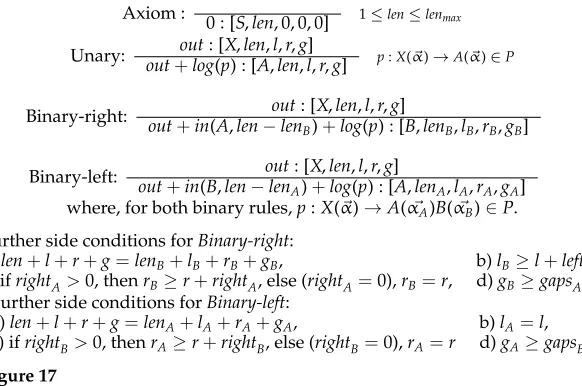
Axiom : 0 : [S,len, 0, 0, 0] 1≤len≤lenmax
Unary: out+outlog: [(pX) : [,lenA,,llen,r,g,]l,r,g] p:X(α)→A(α)∈P
Binary-right: out+in(A,len−outlen: [X,len,l,r,g]
B)+log(p) : [B,lenB,lB,rB,gB]
Binary-left: out: [X,len,l,r,g]
out+in(B,len−lenA)+log(p) : [A,lenA,lA,rA,gA]
where, for both binary rules,p:X(α)→A(αA)B(αB)∈P.
Further side conditions forBinary-right:
a)len+l+r+g=lenB+lB+rB+gB, b)lB≥l+leftA,
c) ifrightA>0, thenrB≥r+rightA, else (rightA=0),rB=r, d)gB≥gapsA.
Further side conditions forBinary-left:
a)len+l+r+g=lenA+lA+rA+gA, b)lA=l,
[image:17.486.63.354.67.260.2]c) ifrightB>0, thenrA≥r+rightB, else (rightB=0),rA=r d)gA≥gapsB.
Figure 17
SX estimate depending on length, left, right, gaps.
The valuein(X,l) for a non-terminalXand a lengthl, 0≤l≤lenmaxis an estimate
of the probability of anXcategory with a span of lengthl. Its computation is specified in Figure 18.
The SX-estimate for a sentence length n and for some predicate C with a range characterized by ρ=l1,r1,. . .,ldim(C),rdim(C) where len= Σidim=1(C)(ri−li) and r= n−rdim(C)is then given by the maximal weight of the item [C,len,l1,r,n−len−l1−r].
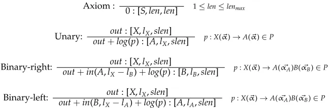
4.3 SX with LR, Gaps, Length
In order to further decrease the space complexity of the computation of the outside estimate, we can simplify the previous estimate by subsuming the two lengthsleftand
rightin a single length lr. The items now have the form [X,len,lr,gaps] with X∈N,
len+lr+gaps≤lenmax,len≥dim(X),gaps≥dim(X)−1.
The computation is given in Figure 19. Again, we define leftA,gapsA, rightA and
gapsB,rightBfor a ruleX(α)→A(αA)B(αB) as before. Furthermore, in bothBinary-left
andBinary-right, we have limitedlrin the consequent item to thelrof the antecedent plus the length of the sister (lenB, resp.lenA). This results in a further reduction of the
number of items while having only little effect on the parsing results.
The SX-estimate for a sentence length n and for some predicate C with a span
ρ=l1,r1,. . .,ldim(C),rdim(C)wherelen= Σdimi=1(C)(ri−li) andr=n−rdim(C)is then the
maximal weight of [C,len,l1+r,n−len−l1−r].
POS tags:
0 : [A, 1] Aa POS tag Unary:
in: [B,l]
in+log(p) : [A,l] p:A(α)→B(α)∈P
Binary: in inB: [B,lB],inC: [C,lC]
B+inC+log(p) : [A,lB+lC]
where eitherp:A(αA)→B(αB)C(αC)∈Porp:A(αA)→C(αC)B(αB)∈P. Figure 18
Axiom : 0 : [S,len, 0, 0] 1≤len≤lenmax
Unary: out+outlog: [(pX) : [,lenA,,lrlen,g,]lr,g] p:X(α)→A(α)∈P
Binary-right: out: [X,len,lr,g]
out+in(A,len−lenB)+log(p) : [B,lenB,lrB,gB] p:X(
α)→A(αA)B(αB)∈P
Binary-left: out+in(B,len−outlen: [X,len,lr,g]
A)+log(p) : [A,lenA,lrA,gA] p:X(
α)→A(αA)B(αB)∈P
Further side conditions forBinary-right:
a)len+lr+g=lenB+lrB+gB b)lr<lrB c)gB≥gapsA
Further side conditions forBinary-left:
[image:18.486.47.403.66.232.2]a)len+lr+g=lenA+lrA+gA b) ifrightB=0 thenlr=lrA, elselr<lrA c)gA≥gapsB
Figure 19
SX estimate depending on length, LR, gaps.
4.4 SX with Span and Sentence Length
We will now present a further simplification of the last estimate that records only the span length and the length of the entire sentence. The items have the form [X,len,slen] withX∈N,dim(X)≤len≤slen. The computation is given in Figure 20. This last esti-mate is actually monotonic and allows for true A∗parsing.
The SX-estimate for a sentence length n and for some predicate C with a span
ρ=l1,r1,. . .,ldim(C),rdim(C)wherelen= Σidim=1(C)(ri−li) is then the maximal weight
of [C,len,n].
In order to prove that this estimate allows for monotonic weighted deductive pars-ing and therefore guarantees that the best parse will be found, let us have a look at the CYK deduction rules when being augmented with the estimate. OnlyUnaryandBinary
are relevant because Scandoes not have antecedent items. The two rules, augmented with the outside estimate, are shown in Figure 21.
We have to show that for every rule, if this rule has an antecedent item with weight
wand a consequent item with weightw, thenw≥w.
Let us start with Unary. To show:inB+outB≥inB+log(p)+outA. Because of the Unaryrule for computing the outside estimate and because of the unary production,
Axiom :
0 : [S,len,len] 1≤len≤lenmax
Unary: out+outlog: [(pX) : [,lXA,slen,l ]
X,slen] p:X(
α)→A(α)∈P
Binary-right: out: [X,lX,slen]
out+in(A,lX−lB)+log(p) : [B,lB,slen] p:X(
α)→A(αA)B(αB)∈P
Binary-left: out+in(B,lout: [X,lX,slen]
X−lA)+log(p) : [A,lA,slen] p:X(
α)→A(αA)B(αB)∈P
Figure 20
[image:18.486.50.378.527.634.2]Unary: inB+outB: [B,ρ]
inB+log(p)+outA: [A,ρ] p:A(
α)→B(α)∈P
Binary: inBin+outB: [B,ρB],inC+outC: [C,ρC]
B+inC+log(p)+outA: [A,ρA]
p:A(ρA)→B(ρB)C(ρC)
is an instantiated rule
(Here,outA,outB, andoutCare the respective outside estimates of [A,ρA], [B,ρB] and [C,ρC].)
Figure 21
Parsing rules including outside estimate.
we obtain that, given the outside estimateoutAof [A,ρ] the outside estimateoutBof the
item [B,ρ] is at leastoutA+log(p), namely,outB≥log(p)+outA.
Now let us consider the ruleBinary. We treat only the relation between the weight of the C antecedent item and the consequent. The treatment of the antecedent B is symmetric. To show:inC+outC≥inB+inC+log(p)+outA. Assume thatlBis the length
of the components of theB item and n is the sentence length. Then, because of the
Binary-right rule in the computation of the outside estimate and because of our in-stantiated rulep:A(ρA)→B(ρB)C(ρC), we have that the outside estimate outC of the C-item is at least outA+in(B,lB)+log(p). Furthermore, in(B,lB)≥inB. Consequently outC ≥inB+log(p)+outA.
4.5 Integration into the Parser
Before parsing, the outside estimates of all items up to a certain maximal sentence length
lenmax are precomputed. Then, when performing the weighted deductive parsing as
explained in Section 3.2, whenever a new item is stored in the agenda, we add its outside estimate to its weight.
Because the outside estimate is always greater than or equal to the actual outside score, given the input, the weight of an item in the agenda is always greater than or equal to the log of the actual product of the inside and outside score of the item. In this sense, the outside estimates given earlier are admissible.
Additionally, as already mentioned, note that the full SX estimate and the SX esti-mate with span and sentence length are monotonic and allow for A∗parsing. The other two estimates, which are both not monotonic, act as FOMs in a best-first parsing context. Consequently, they contribute to speeding up parsing but they decrease the quality of the parsing output. For further evaluation details see Section 6.
5. Grammars for Discontinuous Constituents
5.1 Grammar Extraction
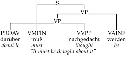
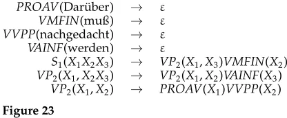
The algorithm we use for extracting an LCFRS from a constituency treebank with cross-ing branches has originally been presented in Maier and Søgaard (2008). It interprets the treebank trees as LCFRS derivation trees. Consider for instance the tree in Figure 22. The S node has two daughters, a VMFIN node and a VP node. This yields a rule
S→VP VMFIN. The VP is discontinuous with two components that wrap around the yield of the VMFIN. Consequently, the LCFRS rule isS(XYZ)→VP(X,Z)VMFIN(Y).
S
VP VP
PROAV VMFIN VVPP VAINF
dar ¨uber muß nachgedacht werden
[image:20.486.49.252.63.156.2]about it must thought be “It must be thought about it”
Figure 22
A sample tree from NeGra.
we have to distinguish these different non-terminals by mapping them to different predicates.
The algorithm first creates a so-called lexical clauseP(a)→εfor each pre-terminal
P dominating some terminala. Then for all other non-terminalsA0 with the children
A1· · ·Am, a clauseA0→A1· · ·Amis created. The number of components of theA1· · ·Am
is the number of discontinuous parts in their yields. The components ofA0are
concate-nations of variables that describe how the discontinuous parts of the yield ofA0 are
obtained from the yields of its daughters.
More precisely, the non-terminals in our LCFRS are allAkwhereAis a non-terminal
label in the treebank andkis a possible fan-out forA. For a given treebank treeV,E,r,l
where Vis the set of nodes,E⊂V×V the set of immediate dominance edges,r∈V
the root node, and l:V→N∪T the labeling function, the algorithm constructs the following rules. Let us assume that w1,. . .,wn are the terminal labels of the leaves
in V,E,r with a linear precedence relationwi≺wj for 1≤i<j≤n. We introduce a
variableXifor everywi, 1≤i≤n.
r
For every pair of nodesv1,v2∈Vwithv2,v2 ∈E,l(v2)∈T, we addl(v1)(l(v2))→εto the rules of the grammar. (We omit the fan-out subscript
here because pre-terminals are always of fan-out 1.)
r
For every nodev∈Vwithl(v)=A0∈/Tsuch that there are exactlymnodesv1,. . .,vm ∈V(m≥1) withv,vi ∈Eandl(vi)=Ai∈/Tfor all
1≤i≤m, we now create a rule
A0(x(0)1 ,. . .,x (0)
dim(A0))
→A1(x1(1),. . .,x (1)
dim(A1)). . .Am(x
(m) 1 ,. . .,x
(m)
dim(Am))
where for the predicateAi, 0≤i≤m, the following must hold:
1. The concatenation of all arguments ofAi,x(1i). . .x (i)
dim(Ai)is the
concatenation of allX∈ {Xi| vi,vi ∈E∗withl(vi)=wi}such that XiprecedesXjifi<j, and
2. a variableXjwith 1≤j<nis the right boundary of an argument of Aiif and only ifXj+1 ∈ {/ Xi| vi,vi ∈E∗withl(vi)=wi}, that is, an
argument boundary is introduced at each discontinuity.
As a further step, in this new rule, all right-hand side arguments of length
PROAV(Dar ¨uber) → ε VMFIN(muß) → ε
VVPP(nachgedacht) → ε
VAINF(werden) → ε
S1(X1X2X3) → VP2(X1,X3)VMFIN(X2)
VP2(X1,X2X3) → VP2(X1,X2)VAINF(X3)
[image:21.486.52.260.64.150.2]VP2(X1,X2) → PROAV(X1)VVPP(X2)
Figure 23
LCFRS rules extracted from the tree in Figure 22.
For the tree in Figure 22, the algorithm produces for instance the rules in Figure 23. As standard for PCFG, the probabilities are computed using Maximum Likelihood Estimation.
5.2 Head-Outward Binarization
As previously mentioned, in contrast to CFG the order of the right-hand side elements of a rule does not matter for the result of an LCFRS derivation. Therefore, we can reorder the right-hand side of a rule before binarizing it.
The following, treebank-specific reordering results in a head-outward binarization where the head is the lowest subtree and it is extended by adding first all sisters to its left and then all sisters to its right. It consists of reordering the right-hand side of the rules extracted from the treebank such that first, all elements to the right of the head are listed in reverse order, then all elements to the left of the head in their original order, and then the head itself. Figure 24 shows the effect this reordering and binarization has on the form of the syntactic trees. In addition to this, we also use a variant of this reordering
Tree in NeGra format:
S VP
NN VMFIN NN AV VAINF
das muß man jetzt machen
that must one now do
“One has to do that now”
Rule extracted for the S node:S(XYZU)→VP(X,U)VMFIN(Y)NN(Z)
Reordering for head-outward binarization:S(XYZU)→NN(Z)VP(X,U)VMFIN(Y) New rules resulting from binarizing this rule:
S(XYZ)→Sbin1(X,Z)NN(Y) Sbin1(XY,Z)→VP(X,Z)VMFIN(Y)
Rule extracted for the VP node:VP(X,YZ)→NN(X)AV(Y)VAINF(Z) New rules resulting from binarizing this rule:
VP(X,Y)→NN(X)VPbin1(Y) VPbin1(XY)→AV(X)VAINF(Y)
Tree after binarization:
S Sbin1
VP
VPbin1
NN VMFIN NN AV VAINF
Figure 24
[image:21.486.54.425.378.652.2]