by Deborah Rumsey, PhD
Intermediate
Statistics
FOR
Intermediate
Statistics
FOR
by Deborah Rumsey, PhD
Intermediate
Statistics
FOR
Intermediate Statistics For Dummies® Published by
Wiley Publishing, Inc.
111 River St.
Hoboken, NJ 07030-5774
www.wiley.com
Copyright © 2007 by Wiley Publishing, Inc., Indianapolis, Indiana Published simultaneously in Canada
No part of this publication may be reproduced, stored in a retrieval system, or transmitted in any form or by any means, electronic, mechanical, photocopying, recording, scanning, or otherwise, except as permit-ted under Sections 107 or 108 of the 1976 Unipermit-ted States Copyright Act, without either the prior written permission of the Publisher, or authorization through payment of the appropriate per-copy fee to the Copyright Clearance Center, 222 Rosewood Drive, Danvers, MA 01923, 978-750-8400, fax 978-646-8600. Requests to the Publisher for permission should be addressed to the Legal Department, Wiley Publishing, Inc., 10475 Crosspoint Blvd., Indianapolis, IN 46256, 317-572-3447, fax 317-572-4355, or online at http:// www.wiley.com/go/permissions.
Trademarks: Wiley, the Wiley Publishing logo, For Dummies, the Dummies Man logo, A Reference for the Rest of Us!, The Dummies Way, Dummies Daily, The Fun and Easy Way, Dummies.com and related trade dress are trademarks or registered trademarks of John Wiley & Sons, Inc. and/or its affiliates in the United States and other countries, and may not be used without written permission. All other trademarks are the property of their respective owners. Wiley Publishing, Inc., is not associated with any product or vendor mentioned in this book.
LIMIT OF LIABILITY/DISCLAIMER OF WARRANTY: THE PUBLISHER AND THE AUTHOR MAKE NO REP-RESENTATIONS OR WARRANTIES WITH RESPECT TO THE ACCURACY OR COMPLETENESS OF THE CON-TENTS OF THIS WORK AND SPECIFICALLY DISCLAIM ALL WARRANTIES, INCLUDING WITHOUT LIMITATION WARRANTIES OF FITNESS FOR A PARTICULAR PURPOSE. NO WARRANTY MAY BE CREATED OR EXTENDED BY SALES OR PROMOTIONAL MATERIALS. THE ADVICE AND STRATEGIES CONTAINED HEREIN MAY NOT BE SUITABLE FOR EVERY SITUATION. THIS WORK IS SOLD WITH THE UNDER-STANDING THAT THE PUBLISHER IS NOT ENGAGED IN RENDERING LEGAL, ACCOUNTING, OR OTHER PROFESSIONAL SERVICES. IF PROFESSIONAL ASSISTANCE IS REQUIRED, THE SERVICES OF A COMPE-TENT PROFESSIONAL PERSON SHOULD BE SOUGHT. NEITHER THE PUBLISHER NOR THE AUTHOR SHALL BE LIABLE FOR DAMAGES ARISING HEREFROM. THE FACT THAT AN ORGANIZATION OR WEBSITE IS REFERRED TO IN THIS WORK AS A CITATION AND/OR A POTENTIAL SOURCE OF FURTHER INFORMATION DOES NOT MEAN THAT THE AUTHOR OR THE PUBLISHER ENDORSES THE INFORMA-TION THE ORGANIZAINFORMA-TION OR WEBSITE MAY PROVIDE OR RECOMMENDAINFORMA-TIONS IT MAY MAKE. FURTHER, READERS SHOULD BE AWARE THAT INTERNET WEBSITES LISTED IN THIS WORK MAY HAVE CHANGED OR DISAPPEARED BETWEEN WHEN THIS WORK WAS WRITTEN AND WHEN IT IS READ.
For general information on our other products and services, please contact our Customer Care Department within the U.S. at 800-762-2974, outside the U.S. at 317-572-3993, or fax 317-572-4002. For technical support, please visit www.wiley.com/techsupport.
Wiley also publishes its books in a variety of electronic formats. Some content that appears in print may not be available in electronic books.
Library of Congress Control Number: 2006939467 ISBN: 978-0-470-04520-6
Manufactured in the United States of America 10 9 8 7 6 5 4 3 2 1
About the Author
Deborah Rumseyhas a PhD in Statistics from The Ohio State University (1993). She is a Statistics Education Specialist/Auxiliary Faculty Member for the Department of Statistics. Dr. Rumsey has been given the distinction of being named a Fellow of the American Statistical Association. She has also won the Presidential Teaching Award from Kansas State University. She is the author of Statistics For Dummies, Statistics Workbook For Dummies,and
Dedication
To my husband Eric: My sun rises and sets with you. To my son Clint: I love you up to the moon and back.
Author’s Acknowledgments
Publisher’s Acknowledgments
We’re proud of this book; please send us your comments through our Dummies online registration form located at www.dummies.com/register/.
Some of the people who helped bring this book to market include the following:
Acquisitions, Editorial, and Media Development
Senior Project Editor: Christina Guthrie
Acquisitions Editors: Kathy Cox, Lindsay Lefevere
Copy Editor: Sarah Westfall
Technical Editor: Phyllis Curtiss, PhD
Editorial Manager: Christine Meloy Beck
Editorial Assistants:Erin Calligan, Joe Niesen, David Lutton, Leeann Harney
Cover Photo: Ingram Publishing
Cartoons: Rich Tennant (www.the5thwave.com)
Composition Services
Project Coordinator: Jennifer Theriot
Layout and Graphics: Brooke Graczyk, Denny Hager, Joyce Haughey, Stephanie D. Jumper
Anniversary Logo Design:Richard Pacifico
Proofreaders: Cynthia Fields, Linda Quigley
Indexer : Dakota Indexing
Publishing and Editorial for Consumer Dummies
Diane Graves Steele, Vice President and Publisher, Consumer Dummies
Joyce Pepple, Acquisitions Director, Consumer Dummies
Kristin A. Cocks, Product Development Director, Consumer Dummies
Michael Spring, Vice President and Publisher, Travel
Kelly Regan,Editorial Director, Travel
Publishing for Technology Dummies
Andy Cummings,Vice President and Publisher, Dummies Technology/General User
Composition Services
Gerry Fahey,Vice President of Production Services
Contents at a Glance
Introduction ...1
Part I: Data Analysis and Model-Building Basics ...7
Chapter 1: Beyond Number Crunching: The Art and Science of Data Analysis ...9
Chapter 2: Sorting through Statistical Techniques ...31
Chapter 3: Building Confidence and Testing Models...49
Part II: Making Predictions by Using Regression...67
Chapter 4: Getting in Line with Simple Linear Regression...69
Chapter 5: When Two Variables Are Better than One: Multiple Regression...87
Chapter 6: One Step Forward and Two Steps Back: Regression Model Selection...107
Chapter 7: When Data Throws You a Curve: Using Nonlinear Regression ...129
Chapter 8: Yes, No, Maybe So: Making Predictions By Using Logistic Regression...149
Part III: Comparing Many Means with ANOVA...159
Chapter 9: Going One-Way with Analysis of Variance...161
Chapter 10: Pairing Things Down with Multiple Comparisons ...177
Chapter 11: Getting a Little Interaction with Two-Way ANOVA ...185
Chapter 12: Rock My World: Relating Regression to ANOVA...195
Part IV: Building Strong Connections with
Chi-Square Tests...207
Chapter 13: Forming Associations with Two-Way Tables ...209
Chapter 14: Being Independent Enough for the Chi-Square Test ...229
Chapter 15: Using Chi-Square Tests for Goodness-of-Fit (Your Data, Not Your Jeans) ...249
Part V: Rebels without a Distribution ...259
Chapter 16: Going Nonparametric ...261
Chapter 17: The Sign Test and Signed Rank Test ...271
Chapter 18: Pulling Rank with the Rank Sum Test ...285
Chapter 19: Do the Kruskal-Wallis and Rank the Sums with Wilcox ...295
Part VI: The Part of Tens ...315
Chapter 21: Ten Errors in Statistical Conclusions...317
Chapter 22: Ten Practice Problems...327
Appendix: Tables for Your Reference ...339
Table of Contents
Introduction...1
About This Book...1
Conventions Used in This Book ...2
What You’re Not to Read ...3
Foolish Assumptions ...3
How This Book Is Organized...4
Part I: Data Analysis and Model-Building Basics ...4
Part II: Making Predictions By Using Regression...4
Part III: Comparing Many Means with ANOVA ...4
Part IV: Building Strong Connections with Chi-Square Tests...5
Part V: Rebels without a Distribution: Nonparametric Statistics...5
Part VI: The Part of Tens ...5
Icons Used in This Book...5
Where to Go from Here...6
Part I: Data Analysis and Model-Building Basics...7
Chapter 1: Beyond Number Crunching: The Art and Science
of Data Analysis . . . .9
Data Analysis: It’s Not Just for Statisticians Anymore ...9
Remembering the old days ...10
The downside of today’s statistical software ...11
Rule #1: Look Before You Crunch...12
Nothing (even a straight line) lasts forever ...12
Data snooping isn’t cool ...13
No (data) fishing allowed ...15
Getting the Big Picture: An Overview of Intermediate Statistics ...19
Population parameter ...19
Sample statistic ...19
Confidence interval ...20
Hypothesis test...21
Analysis of variance (ANOVA) ...22
Multiple comparisons ...23
Interaction effects ...23
Correlation ...25
Linear regression...27
Chi-square tests ...28
Chapter 2: Sorting through Statistical Techniques . . . .31
Qualitative versus Quantitative Variables in Statistical Analysis ...32
Statistics for Qualitative Variables...33
Comparing proportions ...33
Estimating a proportion ...34
Looking for relationships between qualitative variables ...34
Building models to make predictions ...36
Statistics for Quantitative Variables ...37
Making comparisons ...37
Finding connections...38
Making predictions...40
Avoiding Bias ...41
Looking at bias through statistical glasses ...41
Settling the variance controversy: The battle of n–1 versus n...42
Getting Good Precision...44
Understanding precision from a statistical point of view ...44
Measuring precision with margin of error ...45
Making Conclusions and Knowing Your Limitations ...47
Chapter 3: Building Confidence and Testing Models . . . .49
Estimating Parameters By Using Confidence Intervals...50
Getting the basics: The general form of a confidence interval ...50
Finding the confidence interval for a population mean ...51
What changes the margin of error?...53
Interpreting a confidence interval...56
Setting Up and Testing Models...57
What do Ho and Ha represent — really? ...57
Gathering your evidence into a test statistic...58
Determining strength of evidence with a p-value ...59
Deconstructing Type I and Type II errors ...60
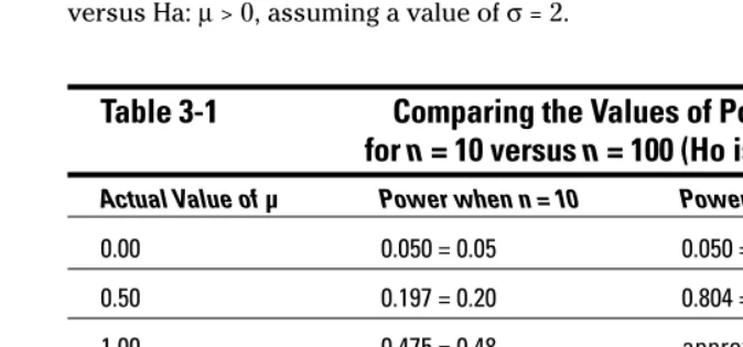
Getting empowered by the power of a hypothesis test ...62
Part II: Making Predictions by Using Regression ...67
Chapter 4: Getting in Line with Simple Linear Regression . . . .69
Exploring Relationships with Scatterplots and Correlations ...70
Using scatterplots to explore relationships...71
Collating the information by using the correlation coefficient ...72
Building a Simple Linear Regression Model ...73
Finding the best-fitting line to model your data ...74
The y-intercept of the regression line...75
The slope of the regression line ...76
Making estimates by using the regression line...76
Intermediate Statistics For Dummies
Checking the Model’s Fit (The Data, Not the Clothes!) ...76
Defining the conditions ...77
Finding and exploring the residuals...78
Using r2to measure model fit...81
Scoping for outliers ...82
Making Correct Conclusions...84
Avoiding slipping into cause-and-effect mode...84
Extrapolation: The ultimate no-no ...85
Knowing the limitations of a simple linear regression model ...86
Chapter 5: When Two Variables Are Better than One:
Multiple Regression . . . .87
The Multiple Regression Model...87
Discovering the uses of multiple regression...88
Looking at the general form of the multiple regression model ...88
Stepping through the analysis ...89
Looking at X’s and Y’s...89
Collecting the data ...90
Pinpointing Possible Relationships ...92
Making scatterplots ...92
Correlations: Examining the bond...93
Checking for Multicolinearity ...95
Finding the Best-Fitting Model...96
Getting the multiple regression coefficients ...97
Interpreting the coefficients ...98
Testing the coefficients...99
Predicting Y by Using the X Variables ...101
Checking the Fit of the Model...102
Noting the conditions ...102
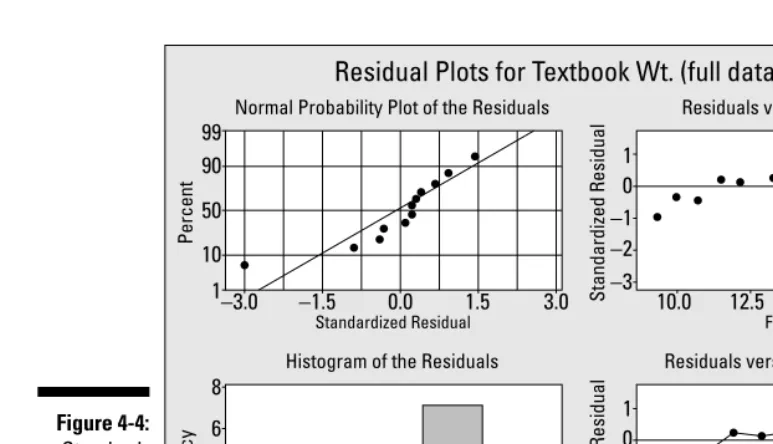
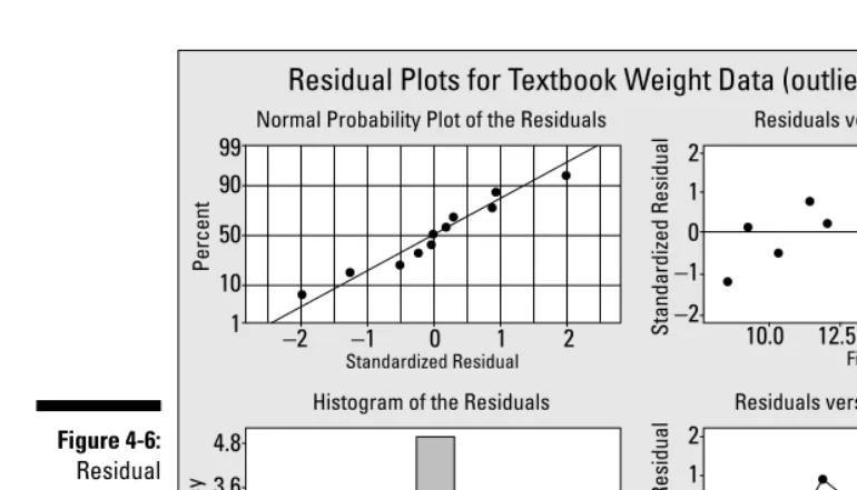
Plotting a plan to check the conditions...102
Chapter 6: One Step Forward and Two Steps Back:
Regression Model Selection . . . .107
Getting a Kick out of Estimating Punt Distance...108
Brainstorming variables and collecting data...108
Examining scatterplots and correlations ...110
Using the Forward Model Selection Procedure...113
Adding variables — one at a time ...113
How well does the model fit? ...115
Applying forward selection to punt distances ...116
Shifting into Reverse: The Backward Model Selection Procedure...118
Eliminating variables one by one ...119
Assessing model fit ...120
Kicking variables out to estimate punt distance...120
xiii
Using the Best Subsets Procedure ...123
Forming all models and choosing the best one...123
Applying best subsets to the punt distance example...124
Comparing Model Selection Procedures...126
Why don’t all the procedures get the same results? ...126
How do the procedures stack up against each other? ...127
Chapter 7: When Data Throws You a Curve: Using
Nonlinear Regression . . . .129
Starting Out with Scatterplots...130
Handling Curves in the Road with Polynomials...131
Bringing back polynomials...132
Searching for the best polynomial model ...134
Using a second-degree polynomial to pass the quiz...135
Assessing the fit of a polynomial model...137
Making predictions...140
Going Up? Going Down? Go Exponential!...142
Recollecting exponential models ...142
Searching for the best exponential model ...143
Spreading secrets at an exponential rate ...145
Chapter 8: Yes, No, Maybe So: Making Predictions By
Using Logistic Regression . . . .149
Setting Up the Logistic Regression Model ...149
Defining a logistic regression model ...150
Using an S-curve to estimate probabilities ...150
Interpreting the coefficients of the logistic regression model ...151
Estimating the chance a movie will be a hit by using logistic regression ...151
General Steps for Logistic Regression...152
Running the analysis in Minitab ...153
Finding the coefficients and making the model...154
Estimating p ...155
Checking the fit of the model...156
Part III: Comparing Many Means with ANOVA ...159
Chapter 9: Going One-Way with Analysis of Variance . . . .161
Comparing Two Means with a t-Test ...162
Evaluating More Means with ANOVA...163
Spitting seeds: A situation just waiting for ANOVA...163
Walking through the steps of ANOVA ...164
Intermediate Statistics For Dummies
Checking the Conditions ...165
Checking off independence...166
Looking for what’s normal ...166
Taking note of spread ...167
Setting Up the Hypotheses...168
Doing the F-Test...168
Running ANOVA in Minitab ...169
Breaking down the variance into sums of squares ...170
Locating those mean sums of squares ...171
Figuring the F-statistic ...172
Making conclusions from ANOVA...173
What’s next? ...175
Checking the Fit of the ANOVA Model ...175
Chapter 10: Pairing Things Down with Multiple Comparisons . . . . .177
Following Up after ANOVA ...177
Pinpointing Differing Means with Fisher and Tukey...180
Fishing for differences with Fisher’s LSD ...180
Separating the turkeys with Tukey’s test ...182
Chapter 11: Getting a Little Interaction with Two-Way ANOVA . . . .185
Setting Up the Two-Way ANOVA Model...186
Determining the treatments ...186
Stepping through the sums of squares...186
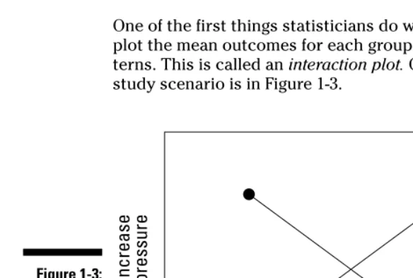
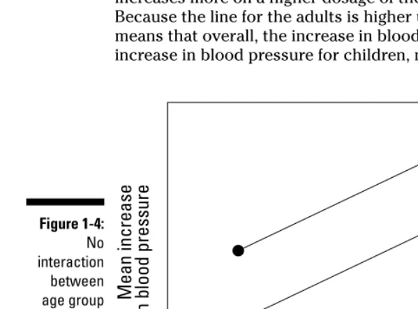
Understanding Interaction Effects ...188
What is interaction anyway?...188
Interacting with interaction plots ...189
Testing the Terms in Two-Way ANOVA...191
Running the Two-Way ANOVA Table...192
Interpreting the results: Numbers and graphs ...192
Chapter 12 Rock My World: Relating Regression to ANOVA . . . .195
Seeing Regression through the Eyes of Variation ...195
Verifying variability in the y’s and looking at x to explain it...196
Seeing the variability in Internet use ...196
Finding an “x-planation” for Internet use ...196
Getting results with regression...198
Assessing the fit of the regression model ...199
Regression and ANOVA: A Meeting of the Models ...200
Comparing sums of squares...201
Dividing up the degrees of freedom ...202
Bringing regression to the ANOVA table ...204
Relating the F- and t-statistics: The final frontier ...205
xv
Part IV: Building Strong Connections with
Chi-Square Tests ...207
Chapter 13: Forming Associations with Two-Way Tables . . . .209
Breaking Down a Two-Way Table ...210
Organizing data into a two-way table ...210
Filling in the cell counts...211
Making marginal totals ...212
Breaking Down the Probabilities...213
Marginal probabilities...213
Joint probabilities ...215
Conditional probabilities...215
Trying to be Independent ...221
Checking for independence between two categories...221
Checking for independence between two variables ...222
Demystifying Simpson’s Paradox ...223
Experiencing Simpson’s Paradox ...224
Asking why: Simpson’s Paradox ...226
Keeping one eye open for Simpson’s Paradox...228
Chapter 14: Being Independent Enough for the Chi-Square Test . . . . .229
A Hypothesis Test for Independence ...230
Collecting and organizing the data...232
Determining the hypotheses...232
Figuring expected cell counts ...233
Checking the conditions for the test ...235
Calculating the Chi-square test statistic...236
Finding your results on the Chi-square table ...238
Drawing your conclusions...241
Comparing Two Tests for Comparing Two Proportions ...243
Getting reacquainted with the Z-test for two population proportions ...244
Equating Chi-square tests and Z-tests for a two-by-two table ...245
Chapter 15: Using Chi-Square Tests for Goodness-of-Fit
(Your Data, Not Your Jeans) . . . .249
Finding the Goodness-of-Fit Statistic ...249
What’s observed versus what’s expected...250
Calculating the goodness-of-fit statistic ...252
Interpreting the Goodness-of-Fit Statistic By Using Chi-Square...254
Checking the conditions before you start...255
The steps of the Chi-square goodness-of-fit test ...256
Intermediate Statistics For Dummies
Part V: Rebels without a Distribution ...259
Chapter 16: Going Nonparametric . . . .261
Arguing for Nonparametric Statistics...261
No need to fret if conditions aren’t met ...262
The median’s in the spotlight for a change...263
So, what’s the catch?...265
Getting the Basics of Nonparametric Statistics ...265
Sign ...266
Rank...267
Signed rank...268
Rank sum ...270
Chapter 17: The Sign Test and Signed Rank Test . . . .271
Reading the Signs: The Sign Test ...271
Testing the median...273
Estimating the median ...275
Testing matched pairs ...278
Going a Step Further with the Signed Rank Test...279
A limitation of the sign test ...280
Stepping through the signed rank test ...280
Losing weight with signed ranks ...282
Chapter 18: Pulling Rank with the Rank Sum Test . . . .285
Conducting the Rank Sum Test ...286
Checking the conditions...286
Stepping through the test...287
Stepping up the sample size ...288
Performing a Rank Sum Test: Which Real Estate Agent Sells Homes Faster?...289
Checking the conditions for this test...290
Testing the hypotheses ...291
Chapter 19: Do the Kruskal-Wallis and Rank the Sums
with Wilcox . . . .295
Doing the Kruskal-Wallis Test to Compare More than Two Populations ...295
Checking the conditions...297
Setting up the test ...299
Conducting the test step by step ...299
Pinpointing the Differences: The Wilcoxon Rank Sum Test...302
Pairing off with pairwise comparisons ...303
Carrying out comparison tests to see who’s different ...303
Examining the medians to see how they’re different ...304
xvii
Chapter 20: Pointing Out Correlations with Spearman’s Rank . . . . .307
Pickin’ On Pearson and His Precious Conditions ...308
Scoring with Spearman’s Rank Correlation ...309
Figuring Spearman’s rank correlation...310
Watching Spearman at work: Relating aptitude to performance ...311
Part VI: The Part of Tens ...315
Chapter 21: Ten Errors in Statistical Conclusions . . . .317
These Statistics Prove . . . ...317
It’s Not Technically Statistically Significant, But . . ...318
This Means X Causes Y ...318
I Assumed the Data Was Normal . . . ...319
I’m Only Reporting “Important” Results ...320
A Bigger Sample Is Always Better ...321
It’s Not Technically Random, But . . ...322
1,000 Responses Is 1,000 Responses ...323
Of Course These Results Apply to the General Population! ...324
I Just Decided to Leave It Out...325
Chapter 22: Ten Practice Problems . . . .327
Comparing Means with One-Way ANOVA...327
Doing Multiple Comparisons ...328
Looking at Two Factors with Two-Way ANOVA ...330
Predicting a Quantitative Variable by Using Regression...331
Predicting a Probability with Logistic Regression ...332
Using Nonlinear Regression for Curved Data ...333
Using Chi-Square to Test for Independence ...335
Checking Specific Models with the Goodness-of-Fit Test ...336
Estimating the Median with the Signed Rank Test...336
Checking Model Fit by Using R2...337
Appendix: Tables for Your Reference . . . .339
t-Table ...339
Binomial Table ...341
Chi-Square Table ...346
Rank Sum Table ...348
F-Table ...349
Index...351
Intermediate Statistics For Dummies
Introduction
R
eady to load your statistical toolbox with a new level of tools?Intermediate Statistics For Dummiespicks up where Statistics For Dummies(or your introductory statistics course) leaves off, and keeps you moving along the road of statistical ideas and techniques in a positive step-by-step way.
The focus of intermediate statistics is on building and testing models based on data. You’re trying to estimate, investigate, correlate, and congregate cer-tain variables based on the information at hand. The process for doing this is two-fold. First you build a model that you think describes your situation (the model-building phase), and then you test your model, using the data you’ve collected (the data analysis phase).
The techniques presented in intermediate statistics are used even more heav-ily in medical and scientific studies than the introductory topics were. The reason is that most real-world studies have more complex problems to solve; they ask more questions and collect more data. Given that the results of these more complex studies are used to make decisions in a host of different areas (including medical science, biology, engineering, business, and politics to name a few) most anyone can benefit from reading this book. You can see applications that give you exposure to real problems and to the process of interpreting and understanding other people’s results.
About This Book
This book is designed for people who want to get into (or at least be able to understand and interpret) some of the more involved techniques in statistics, beyond medians and means, the Central Limit Theorem, and confidence intervals and hypothesis tests. (However, I do add some brief overviews of introductory statistics as needed, just to remind everyone of what was cov-ered and get new readers up to speed.) The topics this time around are many flavors of regression (including simple, multiple, nonlinear, and logistic); ANOVA (one-way and two-way); Chi-square tests (for independence and goodness-of-fit); and nonparametric procedures.
by hand, you often use a computer to get your results. I include instructions for using Minitab to conduct many of the calculations in this book. Most sta-tistics teachers who cover these intermediate topics hold this philosophy as well. (What a relief!)
This book is different from the other intermediate statistics books in many ways, including the following:
Full explanations of intermediate statistical ideas. Many statistics text-books squeeze all the intermediate level topics at the very end of their huge introductory-level textbooks; as a result, these topics tend to get condensed and presented as if they were optional topics. But no wor-ries; I take the time to clearly and fully explain all the information you need to survive and thrive.
Dissection of computer output.Throughout the book, I present many examples that use statistical software to analyze the data. In each case, I present the computer output as well as an explanation of how I got the output and what it means.
An extensive number of examples. I include several examples to cover the many different types of problems you will face.
Lots of tips, strategies, and warnings.I share with you some of the trade secrets, based on my experience teaching and supporting students and grading their papers.
Nonlinear approach.The setup of this book allows you to skip around in the book and still have easy access and understanding of any given topic.
Understandable language.I try to keep things conversational to help you understand, remember, and put into practice statistical definitions, techniques, and processes.
Clear and concise step-by-step procedures.In most chapters, you can find steps that intuitively explain how to work through intermediate sta-tistics problems, and remember how to do it later on.
Conventions Used in This Book
Throughout this book, I’ve used several conventions that I want you to be aware of:
I indicate multiplication by using a times sign, indicated by a lowered asterisk,
*
.I also indicate the null and alternative hypotheses as Ho (for the null hypothesis) and Ha (for the alternative hypothesis).
The statistical software package I use and display throughout the book is Minitab 14, but I simply refer to it as Minitab.
Whenever I introduce a new term, I italicizeit.
Keywords and numbered steps appear in boldface.
Web sites and e-mail addresses appear in monofont.
What You’re Not to Read
At times I get into some of the more technical details of formulas and proce-dures for those individuals who may need to know (or just really want to). These minutiae are marked with a Technical Stuff icon. I also include sidebars as an aside to the essential text, usually in the form of a real-life statistics example or some bonus info you may find interesting. You can feel free to skip those icons and sidebars because you won’t miss any of the main infor-mation you need (but by reading it, you may just be able to impress your stat professor with your above-and-beyond knowledge of intermediate statistics!).
Foolish Assumptions
Because this books deals with intermediatestatistics, I assume you have had one previous course in introductory statistics under your belt (or have at least read Statistics For Dummies [Wiley]), with topics taking you up through the Central Limit Theorem and perhaps an introduction to confidence inter-vals and hypothesis tests (although I review these concepts briefly in Chap-ter 3). Prior experience with simple linear regression isn’t necessary. Only college algebra is needed for the mathematics details. Some experience using statistical software is a plus but not required.
As a student, you may be covering these topics in one of two ways: either at the tail end of your introductory statistics course (perhaps in a hurried way, but in some way nonetheless); or through a two-course sequence in statistics in which the topics in this book are the focus of the second course. If so, this book provides you just the information you need to do well in those courses.
You may simply be interested in intermediate statistics from an everyday point of view or want to add to your understanding of studies and statistical results presented in the media. If this is you, you can find plenty of real-world examples and applications of these statistical techniques in action as well as cautions for interpreting them.
3
How This Book Is Organized
This book is organized into five major parts that explore the main topic areas in intermediate statistics, along with one bonus part that offers a series of quick top-ten references for you to use. Each part contains chapters that break down the part’s major objective into understandable pieces.
Part I: Data Analysis and
Model-Building Basics
This part goes over the big ideas of descriptive and inferential statistics and simple linear regression in the context of model building and decision making. Some material from introductory statistics receives a quick review. I also present you with the typical jargon of intermediate statistics.
Part II: Making Predictions
by Using Regression
Here, you can review and extend the ideas of simple linear regression to that of using more than one predictor variable. This part presents techniques for dealing with data that follows a curve (nonlinear models) and models for yes or no data used to make predictions about whether or not an event will happen (logistic regression). It includes all you need to know about conditions, diag-nostics, model building, data-analysis techniques, and interpreting results.
Part III: Comparing Many
Means with ANOVA
You may want to compare the means of more than two populations. In this case, you use analysis of variance (ANOVA). I discuss the basic conditions required, the F-test, one-way and two-way ANOVA, and multiple comparisons. The final goal of these analyses is to show whether the means of the given populations are different and if so, which ones are higher or lower than the rest.
Part IV: Building Strong Connections
with Chi-Square Tests
This part deals with the Chi-square distribution and how you can use it to model and test qualitative (categorical) data. You see how to test for inde-pendence of two categorical variables using a Chi-square test. (No more spec-ulations just by looking at the data in a two-way table!) You also see how to use Chi-square to test how well a model for categorical data fits.
Part V: Rebels without a Distribution:
Nonparametric Statistics
You can look at techniques used in situations where you can’t (or don’t want to) assume your data comes from a population with a certain distribution. For example, when your population isn’t normal (the condition required by most other methods in intermediate statistics).
Part VI: The Part of Tens
Reading this part can give you an edge in two major areas that go beyond the formulas and techniques of intermediate statistics. Those areas are starting the problem right (knowing what type of problem it is and how to attack it) and ending the problem right (knowing what kinds of conclusions you can and can’t make).
You also find an appendix at the back of the book that contains all the tables you need to understand and complete the calculations used in this book.
Icons Used in This Book
I use icons in this book to draw your attention to certain features that occur on a regular basis. Think of them as road signs that you encounter on a trip. Some signs tell you about shortcuts, but others offer more information that you may need; some signs alert you to possible warnings, while others leave you with something to remember.
When you see this icon, it means I’m explaining how to carry out that particu-lar data analysis using Minitab. I also explain the information you get in the computer output so you can interpret your results.
5
I use this icon to reinforce certain ideas that are critical for success in inter-mediate statistics, such as things I think are important to go over as you prepare for an exam.
This icon points out exciting and perhaps surprising situations where inter-mediate statistics is being used in the real world.
When you see this icon, you can skip over it if you don’t want to get into the nitty-gritty details. They exist mainly for people who have a special interest or obligation to know more about the more technical aspects of the statistical issues.
Tips refer to helpful hints, ideas, or shortcuts that you can use to save time, or alternative ways to think about a particular concept.
I use warning icons to help you stay away from common misconceptions and pitfalls you can face when dealing with intermediate statistics ideas and techniques.
Where to Go from Here
This book is written in a nonlinear way, so you can start anywhere and still be able to understand what’s happening. However, I can make some recom-mendations to those who are interested in knowing where to start.
If you’re thoroughly familiar with the ideas of hypothesis testing and simple linear regression, start with Chapter 5 (multiple regression). Use Chapter 1 if you need a reference for the jargon that statisticians use in intermediate statistics.
If you have covered all topics up through the various types of regression (simple, multiple, nonlinear, and logistic) or a subset of those as your professor deemed important, proceed to Chapter 9, the basics of analysis of variance (ANOVA).
Chapter 14 is the place to begin if you want to tackle qualitative (categorical) variables before hitting the quantitative stuff. You can work with the Chi-square test there.
Nonparametric statistics are presented starting with Chapter 16. This area is a hot topic in today’s statistics courses, yet one that doesn’t seem to get as much space in textbooks as it should. Start here if you want the full details on the most common nonparametric procedures.
Part I
In this part . . .
Chapter 1
Beyond Number Crunching: The
Art and Science of Data Analysis
In This Chapter
Realizing your role as a data analyst
Avoiding statistical faux pas
Delving into the jargon of intermediate statistics
B
ecause you’re reading this book, you’re likely familiar with the basics of statistics. You’re now ready to take it up a notch. That next level involves using what you know, picking up a few more tools and techniques at the intermediate level, and finally putting it all to use to help you answer more realistic questions by using real data.In statistical terms, you’re ready to enter the world of the data analyst.This world’s an exciting one, with many options to explore and many tools avail-able. But, as you may have guessed, you have to navigate this world very carefully, choosing the right methods for each situation. In this book, you can see that I’m including the underlying theories and ideas behind the methods where necessary to help you make good decisions — and not just get into the point-and-click mode that today’s software packages offer.
In this chapter, you review the terms involved in statistics as they pertain to data analysis at the intermediate level. You get a glimpse of the impact that your results can have by seeing what these analysis techniques can do. You also gain insight into some of the common misuses of data analysis and their effects.
Data Analysis: It’s Not Just for
Statisticians Anymore
then were very complicated to use, requiring a great deal of knowledge about statistics to set up and carry out. The calculations were tedious and at times unpredictable and required a thorough understanding of the theories and methods behind the calculations to get correct and reliable answers.
Today, anyone who wants to analyze data can do it easily. Many user-friendly statistical software packages are made expressly for that purpose — Microsoft Excel, Minitab, SAS, and SPSS, just to name a few. Free online programs are even available, such as Stat Crunch, to help you do just what it says — crunch your numbers and get an answer. As you see in this section, the modern easy-to-use statistical packages are good in some ways, and not-so-good in other ways.
The most important idea when applying statistical techniques to analyze data is to know what’s going on behind the number crunching, so you (not the computer) are in control of the analysis. That’s why knowledge of intermedi-ate statistics is so critical.
Remembering the old days
In the old days, in order to determine whether methods gave different results, you had to write a computer program to do it, using code that you had to take a class to learn. You had to type in your data in a specific way that the computer program demanded, and you had to submit your program to a mainframe computer and wait for the printer to print out your results. This method was time consuming and a general all-around pain.
I remember the day in college when I reached bottom. I was just learning to write those sophisticated programs you needed to do the simplest analysis. No matter how hard I tried to write the perfect program, the computer kept spitting my work back at me without doing my analysis, noting error after error in the way I typed the commands. The last straw came when I gave my program to the computer for the umpteenth time: At the end of the printout, the computer told me on the very last line: “Error #34410: Too many errors.”
Now, don’t get the idea that your author doesn’t know what she’s doing. I had all the statistical methods right; I just wasn’t very good at writing computer programs. So for anyone out there who’s ever been frustrated by a computer, I feel your pain, and I try to minimize your troubles throughout this book.
Enough lamenting about having to walk to school uphill both ways in the snow with plastic bags on my feet instead of boots. The point is, statistical software packages have undergone an incredible evolution in the last 10 to 15 years, to the point where you can now enter your data quickly and easily in almost any format. Moreover, the choices for data analysis are well organized
and listed in pull-down menus. Now almost anyone (even me) can quickly see how to find the necessary procedure and tell the computer what to do. The results come instantly and successfully, and you can cut and paste them into a word-processing document without blinking an eye. For example, compar-ing the weight loss for people on different weight-loss programs now takes less than three clicks of the mouse to perform, which is great news for folks like me.
Many very useful and efficient statistical software packages exist, including SAS, SPSS, Data Desk, Stat Crunch, MS Excel, and Minitab, and each one has its own pros and cons (and its own users and protesters). My software of choice, and the one I reference throughout this book, is Minitab, because it’s very easy to use, the results are correct, the output is very clear and profes-sional looking, and the software’s loaded with all the data-analysis techniques that are used in intermediate statistics as well as in this book. While a site license for Minitab can be expensive, the downloadable student version is available for rent for only a few bucks a semester.
The downside of today’s
statistical software
You may be wondering where the downside is in all of this. Is it too good to be true that what was once a tedious, complicated process for analyzing data has now become as easy as checking your e-mail on your cell phone? Yes and no. Yes, it’s too good to be true that the software practically does everything for you — if you don’t pay attention to what the programs are really doing. Yes, it’s too good to be true if you don’t understand that conditions need to be checked in every situation before an analysis should be applied. Yes, it’s too good to be true if you take all the results as complete and utter gospel (as too many statistician wannabees do).
Bottom line: Today’s software packages are too good to be true if you don’t have a clear and thorough understanding of the intermediate level of statis-tics that lie underneath them.
Here’s the good news, though. By reading this book, you gain the understand-ing you need to set you up for success. You get enough of the underlyunderstand-ing intermediate statistical concepts to be empowered, but not be dangerous. You find out what conditions need to be checked on the data before applying an analysis and how to check them. You get a good feel for which analyses to use to answer your question (and which ones can cause you trouble), and you become aware of the kinds of results you can expect. Most importantly, you discover what’s possible and appropriate to conclude from your analysis and what limitations and caveats you need to make.
11
Rule #1: Look Before You Crunch
Many people don’t realize that statistical software can’t tell you when to use and not to use a certain statistical technique. You have to determine that on your own. As a result, people think they’re doing their analyses correctly, but they can end up making all kinds of mistakes. Statistical software packages are centered on mathematical formulas, and mathematical formulas aren’t smart enough to know how you’re applying them or to warn you when you’re doing something wrong (that’s where this book comes in).
In this section, I give some examples of some of the major situations where innocent data analyses can go wrong and why it’s important to know what’s happening behind the scenes from a statistical standpoint before you start crunching numbers.
Nothing (even a straight line)
lasts forever
After you get a statistical equation, or model,that tries to explain or predict some random phenomena, you need to specify for what values the equation applies and for what values the equation doesn’t apply. Equations don’t know when they work and when they don’t; it’s up to the data analyst to determine that. This idea is the same for applying the results of any data analysis that you do.
Bill Prediction is a statistics student, studying the affect of study time on exam score. Based on his experience, and that of a few friends, Bill comes up with the equationy = 10x+ 30, wherey represents the test score you get if you study a certain number of hours (x).This equation is Bill’s model for pre-dicting exam score using study time. Notice that this model is the equation of a straight line with a y-intercept of 30 and a slope of 10.
So Bill predicts, using this model, that if you don’t study at all, you’ll get a 30 on the exam (pluggingx = 0 into the equation and solving for y;this point rep-resents the y-intercept of the line). And he predicts, using this model, that if you study for five hours, you’ll get an exam score ofy = 10
*
5 + 30 = 80. So, the point (5, 80) is also on this line. (I won’t talk in detail at this point about how well Bill’s model does at predicting exam score, but you can just say he’s got some work to do on this and leave it at that for now.)I’m sure you would agree that becausex is the amount of study time, thatx
can never be a number less than zero. If you plug a negative number in for x,
sayx = –10, you gety = 10
*
–10 + 30 = –70, which makes no sense. The worst possible score, according to Bill’s model, is 30, which occurs whenx equals 0.And, you can’t study a negative number of hours, so a negative number forx
itself isn’t even possible.
On the other side of the coin,x probably isn’t a number in the two-digit range (10 or more). Why is this? Say someone did study ten hours for this exam. Plugging in 10 forx in Bill’s equation, you gety = 10
*
10 + 30, which equals 130. Remember,y is the predicted exam score. Because most exams are out of 100 possible points, a score of 130 isn’t possible. (I’m all for extra credit on exams, but 30 points of extra credit is too much, even for me.)The point is that there are limits on the values ofx that make sense in this equation. However, the equation itself,y = 10x+ 30, doesn’t know that, and if you graph this line, it’ll go on forever in both the positive and negative direc-tions (see Figure 1-1).
Data snooping isn’t cool
Statisticians have come up with a saying that you may have heard of: “Figures don’t lie. Liars figure.” Make sure that you find out about all the analyses that were performed on a data set, not just the ones reported as being statistically significant.
Suppose Bill Prediction tries to apply his simple model (from the preceding section) to predict exam scores for his whole class, based on their reported amounts of study time, and he finds out that his results fall flat. He figures out
y
x
5
y=10x+30 50
−50 100
−100 150
−150 200
−200
−5
−10
−15
−20 10 15 20
Figure 1-1:
The liney = 10x + 30, for all possible values of x.
13
that he needs more information, so he tries to uncover what other factors help determine exam score on a statistics test besides study time. Bill mea-sures everything from soup to nuts. His set of possible variables includes study time, GPA, previous experience in statistics, math grades in high school, attitudes toward statistics, whether you listen to classical music while studying, shoe size, whether you chew gum during the exam, and even what your favorite color is (after all, you never know, he figures). For good measure, he includes 11 other variables, for a total of 20 possible factors that he thinks may relate to exam score.
Bill starts out by looking for relationships between each of these variables and exam score, so he does 20 correlations. (Correlation is a measure of the linear relationship between two variables; see the section on correlation later in this chapter). He finds out that four variables have a statistically signifi-cant relationship with exam score (that means the results are supposed to be correct with a 95 percent chance — but only if he collected the data properly and did the analysis correctly).
The variables that Bill found to be related to exam score were study time, math grades in high school, GPA, and whether the person chews gum during the exam. It turns out that his new model fits pretty well (by criteria I discuss in Chapter 5 on multiple linear regression models). Bill now thinks he’s scored a home run and has answered that all-elusive question: How can I do better on my statistics test?
But as they said in Apollo 13,“Houston, we have a problem.” By looking at all possible correlations between his 20 variables and exam score, Bill is actually doing 20 separate statistical analyses. Under typical conditions (I describe these conditions in Chapter 3), each statistical analysis has a 5 percent chance of being wrong just by chance (this value of 5 percent is called the sig-nificance levelof the test).
Because 5 percent of 20 analyses is equal to one, you can expect that when you do 20 statistical analyses, one of them will give the wrong result, just by chance, over the long term. I bet you can guess which one of Bill’s correla-tions likely came out wrong in this case. Of course, study time has nothingto do with exam score, and gum-chewing is the answer to all of our problems, right? (If that were the case, all statisticians would be out of business and working for chewing-gum companies instead.)
What Bill is doing is called data snoopingin the data-analysis business. Bill looks around until he finds something, and then he believes the result. This strategy is dangerous, but one that’s done all too often in the real world. One of the reasons data snooping is running rampant today is because everyone and his brother is out there collecting data and analyzing it — and everyone wants to find something. They’re using statistical software that allows them
to just point and click to do as many analyses as they want, without any warn-ing about what statisticians call the overall error rate(that is, the probability of making an error due to chance during any step of the entire analysis, not just the probability of making an error due to chance on any single analysis).
No (data) fishing allowed
Redoing analyses in different ways to try to get the results you want is called
data fishingin the statistics business, and folks in the stat biz consider it to be a major no-no (however, people unfortunately do it all too often in the name of research).
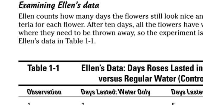
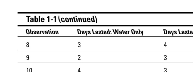
For example, Ellen Go-getter is convinced that dissolving sugar in the water helps cut flowers last longer. She performs an experiment to prove her hypothesis. She cuts two dozen roses and puts one rose in each vase. She fills each vase with 3 cups of water, but in 12 of the vases she adds 1 table-spoon of sugar (the other 12 vases constitute the control group, meaning that Ellen doesn’t apply any new treatment to them to show what happens if she adds nothing). In the next sections, you follow Ellen through her experiment, keeping an eye on the statistical analyses that pop up along the way.
Examining Ellen’s data
Ellen counts how many days the flowers still look nice and uses the same cri-teria for each flower. After ten days, all the flowers have withered to the point where they need to be thrown away, so the experiment is over. You can see Ellen’s data in Table 1-1.
Table 1-1
Ellen’s Data: Days Roses Lasted in Sugar Water
versus Regular Water (Control Group)
Observation Days Lasted: Water Only Days Lasted: Sugar Water
1 3 5
2 3 5
3 4 5
4 4 4
5 4 4
6 4 4
7 3 3
(continued)
15
Table 1-1
(continued)
Observation Days Lasted: Water Only Days Lasted: Sugar Water
8 3 4
9 2 3
10 4 3
11 4 5
12 4 5
Setting the hypothesis
Ellen wants to compare the two methods, water and sugar, to see whether the roses that had sugar added lasted longer than the regular water group. She needs to conduct a hypothesis test whose null hypothesis is Ho: There is no difference in days lasted for sugar group versus control group. Her alter-native hypothesis, which she hopes to show, is Ha: The roses in the sugar group lasted longer than the control group. She figures a two-sample t-test is in order here. (I discuss hypothesis tests in Chapter 3.)
Checking the conditions
Ellen has taken a few statistics classes before and knows that before she plunges into an analysis, she needs to check the proper conditions. For a comparison of two groups, she has to plot the data from each group on a
histogram(a bar graph showing the number of days the flowers lasted, organized into groupings in numerical order versus the number of flowers that lasted each number of days). According to what she knows about a two-sample t-test, the data in each group has to have a normal distribution before she starts. That is, the data has to have a bell-shaped curve when you look at the histogram. Ellen plots the data in histograms for the two groups and gets the following results (see Figures 1-2a and 1-2b).
5 F r equen c y
Days Lasted: Water Only Histogram of Days Lasted: Water Only
4 3 2 1 0 a
2 3 4 5
5 F r equen c y
Days Lasted: SugarGroup Histogram of Days Lasted: SugarGroup
4 7 6 7 6 3 2 1 0 b
2 3 4 5
Figure 1-2: Histograms showing number of days roses lasted, using water only versus sugar added.
Getting the bad news
As you can see in Figures 1-2a and 1-2b, Ellen’s data doesn’t follow the typical bell-shaped curve. One of the problems is her data only takes on values that are positive whole numbers, so numbers like 1.2, 2.3, and the like aren’t pos-sible. (Normal distributions are supposed to have many possible values.) The other problem is that the data has no values outside the typical two-, three-, four-, or five-day range, so the histogram doesn’t have a chance to take on a bell shape. Perhaps more data would have curbed this problem. At any rate, Ellen knows that the conditions for a two-sample t-test aren’t met here; namely that the data doesn’t have a normal distribution and is, in fact,
skewed(meaning set off to one side or the other).
Going nonparametric
Undaunted by this turn of events, Ellen employs a nonparametric test of her data, which is the right thing to do. Statisticians use nonparametric statistics
in situations where the assumptions of the typical analyses aren’t met (like not having a normal distribution). However, nonparametric stats often give more conservative (albeit more accurate) results than the typical (paramet-ric) procedures you’re used to using. (I discuss nonparametrics a bit more in the last section of this chapter. Nonparametric procedures are discussed in full detail in Chapters 16–19.)
Because Ellen’s data doesn’t have a normal distribution or even a symmetric distribution(meaning one that looks the same on each side when you split it down the middle), the mean (or average) isn’t a good measure of the center of the data, so a two-sample t-test isn’t possible. As an alternative, she can test whether the two histograms are the same or not, if she compares the his-tograms of the two populations in question (all roses given water, versus all roses given sugar water).
Because she’s comparing two groups, Ellen uses a Wilcoxon Rank Sum test, also known as the Mann-Whitney test (see Chapter 19). The Wilcoxon Rank Sum test checks whether two populations have the same distribution (mean-ing whether the two histograms look the same) versus one of the populations shifting to the right or left. Ellen’s theory is that the sugar group lasts longer, so she tests Ho: Sugar group and control group have the same distribution versus Ha: Sugar group is shifted to the right of the control group.
Ellen strikes out
To cut to the chase, the Wilcoxon Rank Sum test unfortunately fails to reject Ellen’s null hypothesis. She didn’t prove what she wanted to confirm by her experiment. Not enough roses in the sugar group lasted longer than those roses in the control group. You can see the underlying reason for this result by comparing the medians of the two groups. When you find the median of each of the data sets in Table 1-1, you get the value of 4 in each case. Because the medians of the two data sets are equal, it’s unlikely that Ellen can find a statistically significant result by using this test.
17
Breaking the rules
According to the rules that all good statisticians live by, Ellen’s story should end there. She may still be convinced that sugar indeed helps roses last longer. She may use sugar with her roses for the rest of time and tell her friends to use it too. But, she isn’t allowed to say that sugar water gives sta-tistically different results than water alone; her analysis failed to show that.
But remember, Ellen’s last name is Go-getter, so she’s out to get those results. She knows that nonparametric tests usually give more conservative results than regular tests, and despite the fact that the conditions aren’t met, she decides to analyze her data again, this time using the two-sample t-test.
Putting her data into a two-sample t-test takes only two more clicks of the mouse, and Ellen’s results give her a p-value of 0.043. Using the usual signifi-cance level used for hypothesis tests, 0.050, her p-value is less than this number, so she can reject Ho. (In a two-sample t-test, Ho is that there’s no difference in the means of the two groups. And her Ha in this case is that the mean of the sugar group is larger than the mean of the control group.) So Ellen gleefully cheers herself on for getting the results she wanted and decides there’s no harm in trying a different analysis when all else fails.
Seeing the error of Ellen’s ways
But again, “Houston. . .” — you know the rest. Ellen’s problem is that she cheated her way to getting a result that’s incorrect. She knew that the condi-tions for the two-sample t-test weren’t met, but when the correct analysis failed to get the results she wanted, she found an analysis that did. The trou-ble is, the results of the two-sample t-test are bogus.
Now it may not be a life-and-death situation whether your roses actually do last a little bit longer on sugar or not. (Incidentally, the gardening crowd says they don’t, and that sugar in fact can encourage the growth of stem-clogging bacteria so the flower can’t take in water.) But imagine a situation where doc-tors are trying to test to see whether a certain medication helps people get over an illness faster or whether some procedure helps cancer patients live longer. Now you’re talking about results with a very serious impact.
Using the wrong data analysis for the sake of getting the results you desire results in two major problems:
You mislead your audience into thinking that your hypothesis is actually correct, which it may not be.
Sooner or later someone is going to try to replicate those results and will find out that they can’t be replicated. This discovery will result in a loss of your credibility big time.And unfortunately, you mislead many people in the meantime.
Getting the Big Picture: An Overview
of Intermediate Statistics
Because of the dangers and lingering effects of using the wrong techniques in the wrong situation to analyze data to answer questions, knowing what’s hap-pening behind the scenes of any data analysis and staying within the rules of well-chosen techniques and appropriate practices is very important. In other words, it’s crucial for you to take your knowledge of statistics to the next level.
Intermediate statistics is an extension of introductory statistics, so the jargon follows suit and the techniques build on what you already know. If you’ve been able to grasp the ideas from the first course, you’ll find no trouble with the terminology for intermediate statistics. If you’re still unsure about some of the terms from introductory statistics, you can consult your textbook from your first course or see my other book, Statistics For Dummies(Wiley), for a complete rundown.
In this section, you get an introduction to the terminology you use in interme-diate statistics, and you get a broad overview of the techniques that statisti-cians use for the purpose of analyzing data and the big picture behind them.
Population parameter
A parameteris a number that summarizes the population (the entire group you’re interested in investigating). Examples of parameters include the mean of a population, the median of a population, or the proportion of the popula-tion that falls into a certain category.
Suppose you want to determine the average length of a cell-phone call among teenagers (ages 13 to 18). You’re not interested in making any comparisons; you just want to make a good guesstimate as to what the average time is. So you want to estimate a population parameter (such as the mean or average). The population is all cell-phone users between the ages of 13 and 18 years old. The parameter is the average length of a phone call this population makes.
Sample statistic
You normally can’t study every member of an entire population (how would you like to measure and record the length of every single cell-phone call made by all teenagers?). So you can’t determine population parameters exactly; you can only estimate them. But all is not lost; by taking a sample (a subset of individuals) from the population and studying them, you can come
19
up with a good guess (estimate) of the population parameter, if you play your cards right. A subset of this population is called a sample.A sample statisticis a single number that summarizes that subset of the population.
For example, in the cell-phone scenario, you select a sample of teenagers and measure the length of their cell-phone calls over a period of time (or look at their cell-phone records if you can gain access legally). You take the average of the phone call lengths. For example, the average length of 100 cell-phone calls may be 12.2 minutes — this average is a statistic. This particular statistic is called the sample mean,because it’s the average value from your sample data.
You can also find a statistic called the sample proportion(the proportion of individuals in the sample that have a certain characteristic — for example, the percentage of female teens who use cell phones). Many different statistics are available (which you probably picked up in intro stats) to study different char-acteristics of a sample, such as the median, variance, and standard deviation.
Confidence interval
A confidence intervalis a range of values that provides reasonable estimates for a population parameter. A confidence interval is based on a sample and the statistics that come from that sample. The main reason you want to pro-vide a range of possible values rather than a single number is that sample results vary from sample to sample.
For example, say you want to estimate the percentage of people who eat chocolate. According to the Simmons Research Bureau, 78 percent of adults reported eating chocolate, and of those, 18 percent admitted to eating sweets frequently. What’s missing in these results? These numbers are only a single sample of people, and those sample results are guaranteed to vary from sample to sample. You need some measure of how much you can expect those results to move if you were to repeat the study.
This expected movement in your statistic is measured by the margin of error,
which reflects a certain number of standard deviations of your statistic you add and subtract to have a certain confidence in your results (see Chapter 3 for more on margin of error). If the chocolate-eater results were based on 1,000 people, the margin of error would be approximately 3 percent, meaning the actual percentage of people who eat chocolate in the entire population is expected to be 78 percent, plus or minus 3 percent. In other words, it’s some-where between 75 percent and 81 percent. Now if you only base these results on a sample of 100 people, the margin of error balloons to 10 percent, mean-ing the percentage of chocolate eaters can only be reported to be between 68 and 88 percent. Notice how much wider the interval becomes when a smaller sample size is used. This result confirms that more data means more preci-sion in your results (provided the data is collected properly).
Hypothesis test
A hypothesis testis a statistical procedure that you use to test an existing claim about the population, using your data. The claim is noted by Ho (the null hypothesis). If your data support the claim, you fail to reject Ho. If your data don’t support the claim, you reject Ho and conclude an alternative hypothesis, Ha. The reason most people conduct a hypothesis test is not to merely show that their data support an existing claim, but rather to show that the existing claim is false, in favor of the alternative hypothesis.
The Pew Research Center studied the percentage of people who go to ESPN for their sports news. Their statistics, based on a survey of about 1,000 people, found that in 2000, 23 percent of people said they go to ESPN; while in 2004, only 20 percent reported going to ESPN. The question is this: Does this 3-percent reduction in viewers from 2000 to 2004 represent a significant trend that ESPN should worry about?
To test these differences formally, you can set up a hypothesis test. You set up your null hypothesis as the result you have to believe without your study, Ho = no difference exists between 2000 and 2004 data for ESPN viewership. Your alternative hypothesis (Ha) is that a difference is there.
In very general terms, here’s what’s happening with a hypothesis test. You have the sample data, and you find the statistics that are relevant. In this case, you have two sample percentages, one for 2000 and one for 2004. You take the difference between the two samples (3 percent), and divide it by the standard error for the difference. The standard error measures how much the difference in the statistics is expected to change from sample to sample. In this case, the standard error comes to about 1.8 percent (for specific calcula-tions see Chapter 3).
Taking the difference in the statistics (3 percent = 0.03) divided by the stan-dard error (1.8 percent = 0.018) gives you the value of 1.67 (called the test statistic). This value represents the difference between the two statistics, in terms of number of standard errors. This result has a universal interpreta-tion. Roughly speaking, if your test statistic falls between –2.00 and +2.00, that means the results you found don’t differ enough to get excited about, because 95 percent of the time, this outcome happens just by chance. (And this example falls right into that situation.) After you take the variability of the sample results into account, the difference in these particular samples doesn’t transfer over to the populations they represent. So, because you can’t reject Ho, you have to say the percentage of viewers of ESPN in the entire population probably didn’t change from 2000 to 2004.
Because you have a 95 percent confidence level, this test uses a significance level (αlevel) of 1 – 0.95 = 0.05 or 5 percent. This percentage measures how likely your results would have been just by chance.
21
The trouble is that people often just report the sample statistics and give no regard to the expected amount of change with a new sample. This disregard leads to big mistakes in the conclusions (more on hypothesis testing in Chapter 3).
Analysis of variance (ANOVA)
ANOVA is the acronym for analysis of variance.You use ANOVA in situations where you want to compare the means of more than two populations. For example, you want to compare the lifetime of four brands of tires, in number of miles. You take a random sample of 50 tires from each group, for a total of 200 tires, and set up an experiment to compare the lifetime of each tire, and record it. You have four means and four standard deviations now, one for each data set. But you have different types of variability in your data, each measured by using various sums of squares. (Remember from your intro stats that the variance of a data set is the total of all the squared distances between the data and the mean, all divided by n– 1.)
One of the types of variability in your data is called the variability between
treatments (also known as SST,the treatment sums of squares). SST mea-sures the variation in the average lifetimes of each brand of tire, compared to the overall average lifetime. If SST is large, you have a chance that there’s a difference in lifetimes due to the treatment (in this case, the brand of tire).
Next, you have the variability withinthe treatments (also known as SSE,the error sums of squares). SSE measures the overall average amount of variabil-ity of the tire lifetimes within each particular brand (after all, not all tires are created equal, even if they’re of the same brand). If SSE is large, you have so much variability within the tire brands themselves, that it will be harder to see any real difference between the brands, even if it actually exists.
And finally, you have the totaloverall variability in the data values if you just put them all together into one big data set. This variability is known as SSTO,
the total sums of squares. ANOVA splits up the total variability (SSTO) into the between-groups variability (SST) plus the within-groups variability (SSE).
Then, to test for differences in average lifetime for the four brands of tires, you compare the mean sums of squares for treatments (MST) to the mean sums of squares for error (MSE) in a ratio called the F-statistic.If this ratio is large, then the variability between the brands is more than the variability within the brands, giving evidence that not all the means are the same for the different tire brands. If the F-statistic is small, that means not enough difference was between the treatment means, compared to the general variability within the treatments themselves. In this case, you can’t say that the means are different for the groups. (I give you the full scoop on ANOVA in Chapters 9 and 10.)
Multiple comparisons
Suppose you conduct ANOVA, and you find a difference in the average life-times of the four brands of tire (see preceding section). Your next questions would probably be, which brands are different, and how different are they? To answer these questions, you use multiple-comparison procedures.
A multiple-comparison procedureis a statistical technique that compares means to each other and finds out which ones are different and which ones aren’t. You’re then able to put the groups in order, from those with the largest mean to those with the smallest mean, realizing that sometimes two or more groups were too close to tell and so you put them in the same group.
Suppose you compare the exam scores of four different classes (call them class one, class two, class three, and class four), and your ANOVA procedure finds out that not all the means were the same. That means the F-statistic is large. Next, you use multiple-comparison procedures in order to make sepa-rate comparisons and figure out which classes were about the same and which ones were different, and come up with an ordering of the classes. It may be, for example, that class four was statistically higher than all the others; classes one and two were statistically equivalent, but both were lower than class four. And class one was in a group all by itself at the bottom. The ordering is: class four (highest average), classes two and three (tied for second highest), and class one (the lowest average).
Never take that second step to compare the means of the groups if the ANOVA procedure doesn’t find any significant results during the first step. (See Chap-ter 11 for more information.)
Many different multiple-comparison procedures exist to compare individual means and come up with an ordering in the event that your F-statistic does find that some difference exists. Some of the multiple-comparison procedures include Tukey’s test, LSD, and pairwise t