A Novel Spatial Blind Super Resolution For Video-Sequences
G.George Paul & L.Lakshmi Prasanna Kumar
1(M.Tech )
Electronics and Communication Engineering Department,
G.Pulla Reddy Engineering College, Kurnool,Andhra Pradesh, INDIA
2(ASSISTANT PROFESSOR and M.Tech)
Electronics and Communication Engineering Department,
G.Pulla Reddy Engineering College, Kurnool, Andhra Pradesh, INDIA
[email protected] [email protected]2
Abstract
In Digital image processing the super-resolution of images is a growing technique because of its simple structure with high accuracy as well as reliability is more. As motion fields are having a very high complex nature of motion, so there is need to use the application of super resolution for real life video sequences. The proposed work is implementation for spatial resolution improvement by a novel technique known as blind super resolution(SR),while we unknown about the parameters like noise statistics, point spread function as well as motion fields. In this we estimated the blur by multiscale process but before that we have to upsample the frames with the help of nonuniform interpolation super-resolution. In image if we study details we can know that most of the information present at the edges.So, there is need to first get proper edges of an image. The blur estimation methodology is applied on the few edges but as iteration goes on it is applied to almost all edges of image obtained by gradient. We got more faster convergence in this technique by adopting a pixel domain analysis rather than the filter domain analysis. No of pixel based techniques are there but we preferred Huber-Markov random field because of its very high resolution outputs with preservation of the edges and fine details. It is having two important terms like fidelity and regularization which are analyzed before applying
the random field. The term ‘fidelity’ is continuously
applied weighting by application of masking and the main aim of applying masking is to avoid the inaccurate motion based artifacts. Advantage of proposed work are it can handle complex motion problems, any deformable regions will be estimated accurately, efficient under different brightness condition, detailed structure is obtained as well as it can be applied to fast moving objects. The results obtained are analyzed by subjective and objective analysis to show its state of art over the existing techniques.
Index: Fidelity, Regularization, Super Resolution, Blur Deconvolution, Blind Estimation and Huber Markov Random Field (HMRF).
1. I
NTRODUCTION
spatial density as well as point spread function(PSF).And on other hand temporal resolution is mostly depends on frame rate as well as exposure time required by particular camera.
The basic way to increase the resolution of a video by overlaying the window frame on each frame of the video sequence after that it is checked that which frame is falling inside those frames are combined and formed a new HR frame.
Another example of single video super resolution are given by the learning based, example based and patch based. The main theme for this is small space-time patches from the video sequenece are again and again taken for calculation inside the same or we considered different video for multiple spatio-temporal scales. By doing this high resolution patches are obtained with repeatedly replacing the patches obtained from degraded video.
While estimating blur, the input video is first up-sampled (in case of SR) employing a heterogeneous interpolation or we can say non-uniform interpolation (NUI) SR method, then associate degree repetitious procedure is applied victimization under the given considerations: 1) Throughout the number of iterations, the blur is calculated completely employing a few important edges while weak structures square measure smoothened out, 2) The quantity of contributing edges step by step will increase the chances of getter good performance, 3) structures finer than the blur support can be easily removed or avoided from estimation, 4) the estimation is finished within the filter domain except using pixel domain calculation, finally 5) the estimation is performed at multiple scales to avoid the getting local minima at some points present at edges.
2
.
E
XISTING
M
ETHODS
[1] Visit the below website for more details on SR
http://www.infognition.com/videoenhancer,the
mentioned link will give the following information about the super-resolution used for the enhancement of degraded image as well as videos(which are considered as frames of images).we used video enhancer here to get the more better results for degraded videos using upscaling in the digital videos. That is nothing but increase the resolution of images.
[2] “Limits on super-resolution and how to break them”,by S. Baker and T. Kanade,they also discussed about enhancement of resolution under different conditions of images blurness.in this we worked on two different databases to get the enhanced results.The conversion of image into low and high frequencies will give us the least information also present in image.different types of the constrains are used to get the output with high resolution,in addition we also used reconstruction constrains.
[3]. “Determining optical flow Artificial Intelligence”, given by B.K.P. Horn and B.G. Schunck,in this optical flow cant be calculated locally so we developed second contrains which will calculate the optical flow pattern.It is very helpful to get the image variations which is nothing but where exactly the variation is more and where smoothness of an image is degraded.Brightness level and additive noise in an image will give us the exact where image deformated and applying proposed work we can easily remove those deformations.
recovery of an image that image restoration we are facing the problems like convergence properties, complexity, and other implementation issues.To overcome this type of problems we developed a recent technique known as blind image Deconvolution.Blind in the sense we are not going to consider any references while applying this processing.
[5] “Fundamental limits of reconstruction based super resolution algorithms under local translation”, by the authors Z. Lin and H-Y Shum,as we discussed in all existing techniques there is very less probability of getting success under the condition it should validates the perturbation theorem.so special algorithm is developed to get the better super-resolution compare to existing state of art techniques.
3
.
P
ROPOSED
M
ETHOD
A.
Observation Model
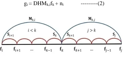
Figure 1: Estimation of total fk frame which are present in LR video sequences
As we observed in above figure, a sliding window (temporal) of length M + N + 1 (with M frames backward and N frames forward) is overlaid around each Low resolution(LR) frame gk of size 𝑁𝑥
𝑔
× 𝑁𝑦 𝑔
× 𝐶, and
all LR frames inside the window can be obtained with the help to generate the HR reference frame fk of size 𝑁𝑥
𝑓
× 𝑁𝑦 𝑓
× 𝐶. Here, Nx and Ny are frame dimensions for
two directions like x and y- directions and C is the number of color channels which is C=3 in color image. The linear forward imaging can be used for the reason of generating a LR frame gi inside the window from the HR frame fk is given by:
𝑔𝑖(𝑥 ↓, 𝑦 ↓; 𝑐) = [𝑚𝑘,𝑖(𝑓𝑘(𝑥, 𝑦; 𝑐)) ∗ ℎ(𝑥, 𝑦)] ↓𝐿
+ 𝑛𝑘,𝑖(𝑥 ↓, 𝑦 ↓; 𝑐), 𝑐 = 1, … , 𝑐,
𝑘 = 1, … 𝑝,
𝑖 = 𝑘 − 𝑀, . . , 𝐾 + 𝑁 (1)
Where, we can say P is the total number of frames, (x↓, y↓) and (x, y) indicate the pixel coordinates in LR and HR image planes respectively, L is given the down sampling factor or SR up scaling ratio (so that 𝑁𝑥
𝑓
=
𝐿𝑁𝑦 𝑔
𝑎𝑛𝑑 𝑁𝑦 𝑓
= 𝐿𝑁𝑦 𝑔
, and ∗ is the two-dimensional convolution operator used in the above formula. According to this model, the HR frame fk is warped with the warping function mk,i , blurred by PSF h, down sampled by L, and finally corrupted by the additive noise nk,i . It is extremely easy to express this linear process in the vector-matrix notion as given by
gi = DHMk,ifk + ni ---(2)
Figure 2. Central motion (blue) versus sequential motion (red).
In (2) fk is the kth HR frame in lexicographical notation indicating a vector of size 𝑁𝑥
𝑓
𝑁𝑦 𝑓
𝐶 × 1, matrices Mk,i and
H are the motion (warping) and convolution operators of size 𝑁𝑥
𝑓
𝑁𝑦 𝑓
𝐶 × 𝑁𝑥 𝑓
𝑁𝑦 𝑓
of size 𝑁𝑥 𝑔
𝑁𝑦 𝑔
𝐶 × 𝑁𝑥 𝑓
𝑁𝑦 𝑓
𝐶, and gi and ni are vectors of the ith LR frame and noise respectively, both of size 𝑁𝑥
𝑔
𝑁𝑦 𝑔
𝐶 × 1.
B. Color Space
The human visual system (HVS) is a smaller amount sensitive to chrominance (color) than to brightness (light intensity). Within the RGB (red, green, blue having three components) color house, all the given three color elements have equal importance so all square measure typically keeps or processed at identical resolution for a pixel. However a lot of economical advantages to take the HVS perception under consideration are by separating the brightness from the colour data and representing luma with higher resolution than vividness present in image.
A popular application to accomplish this separation is to use the YCbCr color house wherever Y is that the luminance part (computed as a weighted average of R, G, and B) and Cb and Cr square measure the blue-difference and red-blue-difference vividness elements. The YUV color space is mostly used for video process algorithms to explain video sequences encoded mistreatment YCbCr color space.
In this proposed work, video sequences will be processed in either RGB or YUV color formats depending on the application. Within the former case, SR is employed to extend the resolution of all R, G, and B channels,but within the latter one, solely the Y channel is processed by SR for quicker computation whereas the Cb and Cr channels are mostly used up scaled to the resolution of the super-resolved Y channel employing a
single-frame up sampling methodology which are already present like linear or Bi-cubiform interpolation. The obtained results associated with given two existing cases are comparable employing a subjective quality assessment.
C. Motion Estimation
Accurate motion estimation (registration of the blur present in image) with sub component exactitude is crucial for video SR to attain an honest performance. 2 completely different approaches are thought-about for registration in video SR: central and serial (Fig. 2). Within the former, motion is directly computed between every system and every one LR frames within its window (Fig. 1). In contrast, within the latter, every frame is registered against its previous frame; then to use with SR, serial motion fields should be reborn to central fields for registration as follows: if Si = [ Sxi, Syi ] is the sequential motion field for the ith frame (w.r.t. the (i −1)th frame), then Mk,i = [ Mxk,i , Myk,i ] , the central motion field for the ith frame when the central frame is the kth frame is obtained as:
𝑀𝑘,𝑖 = − ∑ 𝑆𝑛= −𝑆𝑖+1+ 𝑀𝑘,𝑖+1, 𝑘
𝑛=𝑖+1
𝑘 − 𝑀 ≤ 𝑖 < 𝑘
𝑀𝑘,𝑘= 𝐼
𝑀𝑘,𝑗= ∑ 𝑆𝑛= 𝑆𝑗+ 𝑀𝑘,𝑗−1, 𝑘 < 𝑀 ≤ 𝑖 < 𝑘 + 𝑁 − − − (3) 𝑘
𝑛=𝑖+1
Where, I is the identity matrix.
intervals its reconstruction window. Therefore, the procedure quality and therefore the storage size of the motion fields within the central approach is above that of victimization the successive approach given by this algorithm.
D.
BLUR ESTIMATION
Blur estimation is one of the important step in super-resolution of this proposed work.In a multi-channel BE drawback, the blurs may be calculable accurately alongside the time unit pictures, but in an exceedingly blind SR drawback with a probably completely different blur for every frame, and some ambiguity within the blur estimation is inevitable owing to the down sampling operation for the estimation of blur. In contrast, in an exceedingly blind SR drawback during which all blurs area unit purported to be identical or have gradual changes over time, such associate ambiguity will be avoided [2]. Moreover, as mentioned in Section III-A, the belief of identical (or bit by bit changing) blurs makes it attainable to separate the registration and up sampling procedures from the deblurring method that considerably decreases the blur estimation quality. In Section III-A, the non-uniform interpolations abbreviated as NUI technique to reconstruct the upsampled frame is explained. This upsampled yet-blurry frame is employed to estimate the PSF(s) and therefore the deblurred frames through associate repetitive various diminutions (AM) methods. The blur and frame estimation procedures area unit mentioned in Sections III-B and III-C, severally. The calculable frames area unit used just for the deblurring method so omitted thenceforth. Finally, the general AM improvement method is delineated in Section III-D.
E. Frame up sampling:
In [2] we implemented the things within which the distortion and blurring operations which are present in (2) square measure commutable. Though for videos with arbitrary native motions this commutability doesn't hold specifically for all pixels, but we tend to assume here that this is often around glad. The final word appropriateness of the approximation is valid by the ultimate performance of the formula that's derived supported this model. With this assumption, (2) is rewritten as:
𝐠𝐢= 𝐃𝐌𝐤,𝐢𝐇𝐟𝐤+ 𝐧𝐢= 𝐃𝐌𝐤,𝐢𝐳𝐤+ 𝐧𝐢 (𝟒)
Where 𝐳𝐤= 𝐇𝐟𝐤 is the upsampled but still blurry frame.
Equation (4) shows that we have to construct the upsample frames zk using a proper fusion method and then apply a deblurring method to 𝐳𝐤 to estimate 𝐟𝐤and h.
F. FRAME DEBLURRING
After up sampling the frames, we are going to use the following cost function, J, to estimate the HR frames fk having an estimate of the blur h (or H):
𝑱(𝒇𝒌) = ‖𝝆(𝑯𝒇𝒌− 𝒛𝒌)‖𝟏+ 𝝀𝒏∑‖𝝆(𝛁𝒋𝒇𝒌)‖𝟏 (𝟓) 𝟒
𝒋=𝟏
the observed and simulated LR(low resolution) frames. While in most works the l2-norm is used for the fidelity term, we use the robust Huber norm to better suppress the outliers resulting from inaccurate registration. The next two terms in (5) are used for the different applications like the regularization terms which apply spatiotemporal smoothness to the HR video frames while preserving the edges.
Each element present in the vector function ρ(·) is the Huber function which can be given as,
𝝆(𝒙) = { 𝒙
𝟐 𝒊𝒇|𝒙| ≤ 𝑻
𝟐𝑻|𝒙| − 𝑻𝟐 𝒊𝒇|𝒙| > 𝑇 (𝟔)
The Huber perform ρ(x) could be a umbel-like perform that features a quadratic type for values but or adequate to a threshold T and a linear growth for values bigger than T. The Gibbs PDF of the Huber perform is heavier within the tails than a Gaussian. Consequently, edges within the frames area unit less punished with this previous than with a Gaussian (quadratic) previous.
With the help of a sample vector x, at the nth iteration the non-quadratic Huber-norm ρ(xn)1 is replaced by the following quadratic form which is
‖𝝆(𝑿𝒏)‖
𝟏= (𝑿𝒏)𝑻𝑽𝒏(𝑿𝒏) = ‖𝑿𝒏‖𝑽𝟐𝒏 (𝟕)
Where Vn is the following diagonal matrix given as
𝑽𝒏= 𝒅𝒊𝒂𝒈 ({ 𝟏 𝑿𝒏−𝟏≤ 𝑻
𝑻 𝑿⁄ 𝒏−𝟏 𝑿𝒏−𝟏> 𝑇) (𝟖)
In (8) the dots present above the division and comparison operators indicate element-wise operations. Applying the FP method to (5) and setting the derivative of the cost function with respect to fk to zero results in the following linear equation set:
𝑯𝒏𝑻𝑽𝒏𝑯𝒏+ 𝝀𝒏∑ 𝛁
𝒋𝑻𝐖𝒋𝒏𝛁𝒋= 𝟒
𝒋=𝟏
𝑯𝒏𝑻𝑽𝒏𝒛 𝒌 (𝟗)
Where,
𝑽𝒏= 𝒅𝒊𝒂𝒈 (𝝆(𝑯𝒇 𝒌 𝒏−𝟏− 𝒛
𝒌)) , 𝐖𝒋𝒏
= 𝒅𝒊𝒂𝒈 (𝝆(𝛁𝒋𝒇𝒌𝒏−𝟏)) (𝟏𝟎)
We discussed above how to update the regularization parameter λn at each iteration in Section III-D.
G. Blur estimation:
Within a picture or video frame, non-edge regions and weak structures don't seem to be acceptable for blur estimation. Hence, a lot of correct results would be obtained if the estimation isn't performed in such regions. For this reason, the user ought to 1st manually choose a neighborhood with made edge structure, the foremost salient edges square measure mechanically chosen.
In our proposed work, we tend to use the edge-preserving smoothing technique during which the amount of living edges once smoothing is globally controlled by the regularization constant. This feature is useful once one needs to limit the amount of salient edges at every iteration. This smoothing technique aims to stay associate degree meant variety of non-zero gradients through l0 gradient diminution victimization the subsequent value function:
𝑱(𝒇𝒌′𝒏) = ‖𝒇𝒌′𝒏− 𝒇𝒌𝒏‖𝟐 𝟐
+ 𝜷𝒏(‖𝛁
𝒙𝒇′‖𝟎+ ‖𝛁𝒚𝒇′‖𝟎) (𝟏𝟏)
# (i| xi = 0). Unlike shock filtering, this smoothing method does not need pre-filtering of noise.
Though adequate edge pixels area unit needed for correct blur estimation, it's shown in one of the given references that structures with scales smaller than the FTO support might hurt blur estimation. Galvanized by that employment, we have a tendency to outline Rkn in (12) to live the quality of every constituent for blur estimation:
𝑹𝒌𝒏= |𝑨𝑩𝒇𝒌′𝒏| (𝟏𝟐)
Where A and B are the basic convolution operators for the spatial filters a and b, respectively, as defined below:
𝒂 = [ 𝟏 … 𝟏 ⋮ ⋱ ⋮ 𝟏 … 𝟏
] (𝟏𝟑)
𝒃 = 𝛁𝒙+ 𝛁𝒚= [−𝟏𝟐 −𝟏𝟎] (𝟏𝟒)
In (13) and (14), there is that the all-ones filter of size 11*11 and b is that the sum-of-gradients filter. As we used to compute R_k^n, the total of gradient elements of f_k^n is computed initial, then at every element it's summed up with the values of all neighboring pixels, and eventually its definite quantity is obtained. For pixels on slender structures, the total of gradient values cancels out one another. Therefore, R_k^n sometimes incorporates a tiny worth at the situation of slender edges and sleek regions. Then f_k^n is refined by solely holding robust and non-spike edges:
𝛁𝒇𝒌′′𝒏= {𝛁𝒇𝒌 ′𝒏 𝒊𝒇|𝛁𝒇
𝒌 ′𝒏| > 𝑻
𝟏 𝒏𝒂𝒏𝒅 𝐑
𝒌 𝒏> 𝑻
𝟐 𝒏
𝟎 𝒐𝒕𝒉𝒆𝒓𝒘𝒊𝒔𝒆 (𝟏𝟓) Algorithm 1 Blur Estimation Procedure
Require: 𝑔1,…..,𝑔𝑝,𝜆𝑚𝑖𝑛, Υ𝑚𝑖𝑛 and initials ℎ𝑜. 𝜆𝑜. 𝛾𝑜. 𝛽𝑜. 𝑇1𝑜, 𝑇20
Set n: =0 % Am loop iteration number S: = # of scales
Use luma or one color channel of 𝑔1,…..,𝑔𝑝1
for k: =1 to 𝑃1do % Loop on 𝑷𝟏reference frames
if L>1 then % For SR reconstruction 𝑧𝑘= 𝑁𝑈𝐼(𝑔𝑘−𝑀, … . , 𝑔𝑘+𝑁)
else % For BD reconstruction 𝑧𝑘= 𝑔𝑘
end if
𝑓0𝑘= 𝑧𝑘
%HR frame and blur estimation
for s: =1 to S do % Multi-scale approach Rescale 𝑧𝑘, 𝑓𝑘𝑛 𝑎𝑛𝑑 ℎ𝑛
% AM loop iteration
while “AM stopping criterion “is not satisfied do n=n+1
% Updating procedure for f compute 𝐕𝐧and 𝐖
𝑗𝑛 using (10)
update 𝜆𝑛
while𝐟𝑛 does not satisfy “CG stopping criterion” do
𝑓𝑘𝑛: = CG iteration for system in (9); starting at
𝑓𝑘𝑛−1
end while
Apply constraints on 𝑓𝑘𝑛
% Updating procedure for 𝒉𝒏
Update 𝛾𝑛. 𝛽𝑛. 𝑇 1𝑛 𝑎𝑛𝑑 𝑇2𝑛
Compute the smoothed frame 𝑓𝑘𝑚 from (11)
Compute ∇𝑓𝑘′′𝑛 from (15)
Edge tapping of ∇𝑓𝑘′′𝑛
Compute ℎ𝑘𝑛(𝑥, 𝑦) from (17)
Apply constraints on ℎ𝑛
Where 𝑻𝟏𝒏 and 𝑻𝟐𝒏 are threshold parameters which
decrease at each iteration.To avoid ringing artifact, we apply the MATLAB function edgetaper() to ∇𝑓𝑘𝑛. Then we estimate each blur hk using the cost function J(h) below: 𝑱(𝒉) = ∑‖𝛁𝒛𝒌− 𝛁𝑭𝒌′′𝒉‖𝟐 𝟐 + 𝜸𝒏‖𝛁𝒉‖ 𝟐 𝟐 (𝟏𝟔) 𝑷𝟏 𝒌=𝟏
Where P1 ≤ M + N and 𝑭𝒌 is the convolution
matrix of fk. Since J(h) in (16) is quadratic, it can be easily minimized by pixel-wise division in the frequency domain [41] as:
𝒉𝒌𝒏(𝒙, 𝒚) = 𝓕−𝟏 ( ∑ ∑ { [𝓕(𝛁𝒊) ×̇ 𝓕(𝒇̇ 𝒌′′𝒏) ̅̅̅̅̅̅̅̅̅̅̅̅̅̅̅̅̅̅̅̅ ×̇ (𝓕(𝛁𝒊) ×̇ 𝓕(𝒛̇ ̇ 𝒌)) ] ̇ [|𝓕(𝛁𝒊) ×̇ 𝓕(𝒇̇ 𝒌′′𝒏)| 𝟐̇ + 𝜸𝒏|𝓕(𝛁 𝒊)|𝟐̇] } 𝟐 𝒊=𝟏 𝑷𝟏 𝒌=𝟏 ) (𝟏𝟕)
Where ∇i(i = 1, 2) is ∇x or ∇y, F(·) and F−1(·) are FFT and inverse-FFT operations, and (·) is the complex conjugate operator. We then applied the known constraints for PSF: its negative values are set to zero, then the PSF is normalized to the range [0, 1], and centered which is in support window.
H. Overall Optimization for Blur Estimation:
The overall optimization procedure which is aimed for estimating the PSF is shown in Algorithm 1. The HR frames and the PSF are sequentially updated within the AM iterations shown in the algorithm. We use a multi-scale approach to avoid trapping in local minima. The regularization coefficients 𝝀𝒏 in (9) and𝜸𝒏 in (17)
decrease at each AM (alternating minimization) iteration up to some minimum values 𝝀𝒎𝒊𝒏 and 𝜸𝒎𝒊𝒏, respectively
(see [2] for a discussion). The variation of these coefficients is given by:
𝝀𝒏= 𝒎𝒂𝒙(𝒓𝝀𝒏−𝟏, 𝝀
𝒎𝒊𝒏) , 𝜸𝒏
= 𝒎𝒂𝒙(𝒓𝜸𝒏−𝟏, 𝜸
𝒎𝒊𝒏) (𝟏𝟖)
Where r is a scalar less than 1. Also the values of βn in (11) and Tn 1 and T2n in (15) fall at each AM iteration which increases the number of contributing pixels to blur estimation as the optimization proceeds.
IV. FINAL HR FRAME ESTIMATION
After completion of the PSF estimation, the final HR frames are reconstructed through minimizing the following cost function as given below,
𝑱(𝒇𝟏, … … , 𝒇𝒑) = ∑ ( ∑ ‖𝝆 (𝒐𝒌,𝒊(𝑫𝑯𝑴𝒌,𝒊𝒇𝒌𝟏− 𝒈𝒊))‖ 𝟏 𝑲+𝑵 𝒊=𝒌−𝑴 𝑷 𝒌=𝟏 + 𝝀 ∑‖𝝆(𝛁𝒋𝒇𝒌)‖𝟏 (𝟏𝟗) 𝟒 𝒋=𝟏 )
Where Ok,i is a diagonal weighting matrix that assigns less weights to the outliers. Minimizing this cost function with respect to fk yields:
( ∑ 𝑴𝒌,𝒊𝑻𝑯𝑻𝑫𝑻𝒐𝒌,𝒊𝑽𝒏𝑫𝑯𝑴𝒌,𝒊+ 𝝀 ∑ 𝛁𝒋𝑻𝑾𝒏𝛁𝒋 𝟒 𝒋=𝟏 𝑲+𝑵 𝒊=𝑲−𝑴 ) 𝒇𝒌𝒏 = 𝑴𝒌,𝒊𝑻 𝑯𝑻𝑫𝑻𝒐𝒌,𝒊𝑽𝒏𝒈𝒊 (𝟐𝟎) Where, 𝑽𝒏= 𝒅𝒊𝒂𝒈 (𝝆(𝑫𝑯𝑴 𝒌,𝒊𝒇𝒌𝒏−𝟏− 𝒈𝒊)) , 𝐖𝒋𝒏 = 𝒅𝒊𝒂𝒈 (𝝆(𝛁𝒋𝒇𝒌𝒏−𝟏)) (𝟐𝟏)
and the m-th diagonal element of Onk,i is computed according to below equation:
𝒐𝒌,𝒊[𝒎] = 𝒆𝒙𝒑 {
‖𝑹𝒎(𝝆(𝑫𝑯𝑴𝒌,𝒊𝒇𝒌𝒏−𝟏− 𝒈𝒊))‖
𝟐𝝈𝟐 } (𝟐𝟐)
The final frame estimation algorithm is shown in below Algorithm 2.
4.
S
IMULATION
R
ESULTS
The proposed work is shown by MATLAB implementation. We compared proposed work with existing super-resolution technique and shown that state of art of the proposed work is better compare to existing techniques for super-resolution. We used here bicubic as existing technique to show the advantages of PSNR for proposed work compare to existing technique.
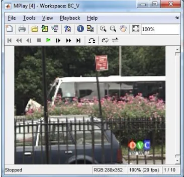
Figure 1: Degraded Video Sequence as an input
In input video there may be different types of degradation like fog, blurness which we have to estimate for enhancement. our proposed algorithm is considered for three types of degradations.
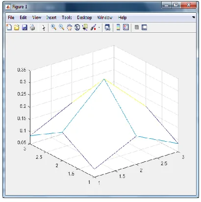
Figure 2: Motion Estimation in Video Sequence Algorithm 2 Final Frame Estimation Procedure
Require: 𝑔1,…..,𝑔𝑝, and 𝜆
1: Set n: = 0 % FP loop iteration number
2: for k: =1 to P do % Loop on P reference frames
3: Estimate sequential motion fields 𝑆1, … . , 𝑆𝑝
4:Compute central motion fields 𝑀1, … . . 𝑀𝑝 using (??)
5:Estimate the blur h using Algorithm 1 7:% Estimate HR frames using FP loops
8:while ‘’FP stopping criterion” is not satisfied do
9: n=n+1
10: Compute 𝐎𝑘𝑗𝑛 using (22)
11: Compute 𝐕𝑛and 𝐖
𝑗𝑛 using (21)
12: While𝑓𝑛 does not satisfy “”CG stopping criterion” do
13:𝑓𝑘𝑛 : = CG iteration for system in (20); starting at 𝑓𝑘𝑛−1
14: end while
15 Apply constraints on 𝑓𝑘𝑛
17: end while
Motion estimation in the degraded video is done because we want to process the finest elements present in an image which are finest that blur also.
Figure 3: Inverse Video Sequence
Here, we calculated inverse video sequences to get accuracy and this type processing will takes place iteratively. Previously it is calculated at some edges but later it is calculated for all edge gradient.
Figure 4: Bi-Cubic Interpolation Method
Bi-cubic interpolation is applied to get the super resolution for single frame upsampling method.We converted Image which is in RGB format to YCbCr format and normally we applied upsampling to Cb and Cr plane but the intensity plane Y is upsampled by using Bi-cubic method.
Figure 5: Proposed Method Video Sequence
Video is considered as sequence of frames and we applied proposed work on degraded video sequence to estimate blur and to remove it. So finally we got these results. We estimated the blur by multiscale process but before that we have to upsample the frames with the help of nonuniform interpolation super-resolution.
5.
C
ONCLUSION
techniques. First we applied the non-uniform interpolation (NUI) super resolution to up sample the frames under consideration that the blur is nothing but it’s having slow variations as time proceed or it may be identical. From this upsample frames blur is estimated by iterative processing on important edges. Finally we reconstructed frames which are blur estimated by application of non blind super resolution is performed iteratively. Masking is applied to suppress the artifacts present due to inaccurate motion estimation. The subjective are well as objective analysis for obtained results will show that the state of art for implementation. Comparative study will show the superior performance of proposed work.
R
EFERENCES
[1] Visit the below website for more details on SR http://www.infognition.com/videoenhancer/,
[2] “Limits on super-resolution and how to break them”,by S. Baker and T. Kanade, IEEE Transaction on Pattern Analysis Machine Intelligence.
[3]. “Determining optical flow Artificial Intelligence”, given by B.K.P. Horn and B.G. Schunck
[4] “Blind image deconvolution”by the authors D. Kundur and D. Hatzinakos in IEEE Signal Processing Magazine.
[5] “Fundamental limits of reconstruction based superresolution algorithms under local translation”, by the authors Z. Lin and H-Y Shum in IEEE Transaction on Pattern Analysis Machine Intelligence.
[6] “A bayesian approach to adaptive video super resolution”,by the authors C. Liu and D. Sun. in IEEE International Conference on Computer Vision and Pattern Recognition, 2011.
[7] “Automatic estimation and removal of noise from a single image”. By the authors C. Liu, R. Szeliski, S. B. Kang, C. L. Zitnick, and W. T. Freeman in IEEE Transaction on Pattern Analysis Machine Intelligence,
[8] “Fast image/video upsampling. ACM Transactions on Graphics” (Proceedings of ACM SIGGRAPH), by the authors Q. Shan, Z. Li, J. Jia, and C-K Tang.