A Method for Hemispherical Ground Based Remote Sensing of Urban Surface Temperatures

Scholarship@Western

Scholarship@Western

Electronic Thesis and Dissertation Repository

6-2-2017 12:00 AM

A Method for Hemispherical Ground Based Remote Sensing of

A Method for Hemispherical Ground Based Remote Sensing of

Urban Surface Temperatures

Urban Surface Temperatures

Michael A. Allen

The University of Western Ontario

Supervisor

Dr. James A Voogt

The University of Western Ontario

Graduate Program in Geography

A thesis submitted in partial fulfillment of the requirements for the degree in Master of Science © Michael A. Allen 2017

Follow this and additional works at: https://ir.lib.uwo.ca/etd

Part of the Climate Commons

Recommended Citation Recommended Citation

Allen, Michael A., "A Method for Hemispherical Ground Based Remote Sensing of Urban Surface Temperatures" (2017). Electronic Thesis and Dissertation Repository. 4594.

https://ir.lib.uwo.ca/etd/4594

This Dissertation/Thesis is brought to you for free and open access by Scholarship@Western. It has been accepted for inclusion in Electronic Thesis and Dissertation Repository by an authorized administrator of

This thesis presents a method for deriving time-continuous urban surface temperature and heat island assessments from hemispherical ground-based measurements of upwelling thermal radiation. The method, developed to overcome geometric and temporal biases inherent in traditional thermal remote sensing of urban surface climates, uses a sensor view model in conjunction with a radiative transfer code to derive atmospherically corrected, hemispherical radiometric urban surface temperatures. These are used to derive two long-term climatologies of surface urban heat island (sUHI) magnitudes for Basel, Switzerland and Vancouver, Canada. sUHI development shows significant variation based on time-of-day, season, and ambient and synoptic conditions. Results also show large differences in remote sensed sUHI from

hemispherical, nadir and complete representations of the urban surface, with a nadir view overestimating seasonal sUHImaxfrom a complete view by nearly a factor of two. In contrast, a

hemispherical view provides significantly more representative, time-continuous urban surface temperature and sUHI analysis.

Keywords: urban, climate, surface, temperature, thermal, remote sensing, micrometerology, urban heat island

Thank you to my research advisor, Dr. James Voogt for his constant encouragement and trust in me through this project, for putting up with my odd work schedules and round the clock emails, and for refocusing and reining me in at times. I am tremendously grateful for his

support and for giving me the opportunity to talk about my graduate work all over the world. Thank you for a great two years.

Thank you to A. Christen who provided a good portion of the foundational work that made this thesis possible.

Thank you to C. Smart, who served on both my committee and examination board, for his excitement and insight about this work. Thanks are also due to the other members of my examination board, J. Wang and G. Osinski, for their prompt and thoughtful comments.

Thank you to my family for their love and support and for reminding me that my audience isn’t always climatologists.

Thank you to my work study student M. Bourke, who spent quite a few weekends in the lab running data for me - without which, this thesis would not have been completed on time.

Thank you to my lab-mates D. Kuruklaarachchi, T. Wiechers, and R. Hilland, and quasi-lab-mates J. Howett, L. Middleton, C. Irwin, and N. Pearce for their wonderful Canadian hospitality and for at times keeping me sane. Thanks also to S. Cappuccitti, S. Pearce, K. West, V. Staples, J. Williams, R. Davis, B. Holmes, and T. Eckmann.

In truth, this space is too small to thank everyone I would like to. To those who

contributed to this work in any capacity - directly or indirectly - thank you. You know who you are.

The body of this thesis (Chapters2and3) is made up of two academic papers with the following authorship:

1. An atmospheric correction method to derive hemispherical time-continuous urban surface temperature

• Michael A. Allen: 60%, Developed the method, its parameterization, and evaluations for both. Contributions to method theorization. Produced text and figures (unless otherwise referenced).

• James A. Voogt: 30%, Project conceptualization. Contributions to methodology and development. Edited text and figure design.

• Andreas Christen 10%, Project conceptualization. Provided data.

2. A climatology of sUHI derived from hemispherical radiometric surface temperatures

• Michael A. Allen: 70% Conducted exploratory data analysis and determined the analysis to present. Produced results, text, and figures (unless otherwise referenced).

• James A. Voogt: 20% Contributions to interpretation of results. Edited text and figure design.

• Andreas Christen 10% Contributions to interpretation of results and figure design. Provided data.

List of Tables ix

List of Figures xi

List of Symbols xviii

1 Introduction 1

1.1 Biases and shortcomings in thermal remote sensing of urban Tsurf . . . 6

1.2 Research questions and objectives . . . 11

References . . . 13

2 An atmospheric correction method to derive hemispherical time-continuous urban

surface temperature 16

2.1 Introduction . . . 16

2.2 Atmospheric effects on TIR radiation . . . 18

2.2.3 Atmospheric correction of near-ground TIR radiation . . . 24

2.3 A ”rolling lookup table” method for hemispherical atmospheric correction . . . . 27

2.3.1 Study area. . . 28

2.3.2 Modeling path lengths of 3-dimensional terrain . . . 34

2.3.3 Modeling hemispherical irradiances . . . 35

2.4 Evaluation of the method using profiles of upwelling longwave radiation over a homogeneous flat surface . . . 39

2.5 Results. . . 43

2.5.1 Atmospheric correction magnitudes . . . 43

2.6 Comparing Tsurffrom different sensor geometries . . . 50

2.7 Discussion. . . 53

2.7.1 Controls on atmospheric correction magnitude . . . 53

2.7.2 The effect of non-uniform pyrgeometer spectral dome transmittance on correction magnitudes . . . 54

2.7.3 The effect of sensor sampling geometry on remote sensed Tsurf . . . 58

2.8 Sensor placement sensitivity testing . . . 59

2.9 A practical parameterization . . . 67

2.10 Conclusions . . . 70

tures 77

3.1 Introduction . . . 77

3.1.1 Bias in thermal remote sensing . . . 79

3.2 Methods . . . 82

3.2.1 A method to retrieve hemispherical radiometric urban Tsurf . . . 82

3.2.2 Method evaluation and sensitivity testing . . . 84

3.2.3 A parameterization scheme . . . 85

3.2.4 Study area. . . 86

3.2.5 sUHI analysis . . . 90

3.3 Results. . . 92

3.3.1 Diurnal and seasonal variability in sUHI magnitudes . . . 92

3.3.2 The effect of sensor-surface geometry on sUHI . . . 99

3.3.3 The effect of meteorological conditions on sUHI . . . 101

3.3.4 The effect of rural/non-urban characteristics on sUHI . . . 111

3.4 Discussion. . . 113

3.4.1 Diurnal patterns of sUHI . . . 113

3.4.2 Seasonal patterns of sUHI . . . 118

3.4.3 Sensor-surface-sun geometries and sUHI . . . 119

3.4.4 Meteorological controls on sUHI. . . 121

4 Conclusion 131

4.1 Summary of results . . . 131

4.2 Limitations and future work . . . 134

4.3 Final remarks . . . 136

References . . . 137

A Transmittances for a range of water vapor mass densities and path lengths. 139

2.1 Weights applied to individual facet temperature components in to calculate

com-plete and nadir temperatures for the Basel Sperrstrasse street canyon. . . 34

2.2 Statistical performance of the Payerne evaluation. RMSEsand RMSEurepresent

the systemic and unsystematic RMSE respectively. The arrangement of

statisti-cal tests were selected from Willmott et al. (1985) and Willmott et al. (2012). n

= 378 . . . 43

2.3 Planck weighted mean sensor response and Tbias for a suite of common urban

emission temperatures. . . 56

2.4 Statistical performance of Themderived using the parameterization scheme

rela-tive to modeled Them,r. RMSEsand RMSEurepresent the systemic and

unsystem-atic RMSE respectively. The arrangement of statistical tests were selected from

Willmott et al. (1985) and Willmott et al. (2012). n = 853 . . . 69

3.1 A description of morphological parameters and measured variables for BUBBLE

urban and rural sites. Modified from Rotach et al. (2005) to include only relevant

urban and rural sites. . . 90

3.3 A summary of the relationship between sUHI, meteorological variables, and clUHI. These relationships are generalizable and represent the character of mean diurnal sUHI in response to changing conditions. . . 124

A.1 A look-up table of bulk, point to point atmospheric transmittances as a function of path length (m) and water vapor mass density (g m−3_{). Assembled from} sim-ulations in MODTRAN 4.1 with Tair= Tsurf=300 K, CO2= 400ppm, and trace absorber and O3 concentrations supplied by the mid-latitude summer standard atmospheric profile (Kantor and Cole, 1962) . . . 140

A.2 Continued from Table A.1 . . . 141

A.3 Continued from Table A.2 . . . 142

A.4 Continued from Table A.3 . . . 143

A.5 Continued from Table A.4 . . . 144

1.1 Projected FOVs for a narrow-FOV sensor at nadir and oblique angles, and a

wide-FOV hemispherical sensor viewing an idealized urban array with building

widthW, height 2W, and inter element spacing W. Figure from Adderley et al.

(2015) under a Creative Commons Attribution 4.0 License. . . 7

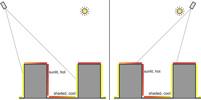
1.2 A narrow-FOV sensor viewing an idealized urban surface from two angles. Left:

viewing the surface approximately perpendicular to the sun’s angle. Right:

view-ing the surface approximately parallel to the sun’s angle. The two viewview-ing angles

yield different remote sensed Tsurfby sampling different arrangements of sunlit

and shaded features. Both will deviate from an area weighted ”complete” urban

Tsurf. . . 8

2.1 At-sensor spectral directional radiances computed in MODTRAN 4.1 (Berk et

al., 1987) for short (30m) and long (3000m) path lengths (z) with Planck curves

indicating spectral radiances at Tsurf= 300Kand Tair= 290K. . . 19

2.2 Spectral transmission of water vapor as a function of height. Model results from

MODTRAN 4.1 for radiance emitted from a planar surface at 300Kthrough an

atmosphere with water vapor content of 8g m−3_{. Sampled at heights of 1, 5, 10,} 15, 20, 25, and 30m. . . 21

over an idealized 2-dimensional urban area. . . 25

2.4 A workflow schematic depicting the input, model, and output-processing steps

of a ”rolling lookup table method” for hemispherical radiometric surface

tem-perature retrial. . . 28

2.5 The BUBBLE study site in Basel, Switzerland with urban and rural site locations

indicated. . . 30

2.6 A schematic showing the TIR radiation instrument setup at the Sperrstrasse urban

canyon. Pyrgeometer locations and IRT FOVs for roof, wall, and road facets are

indicated. Only instruments relevant to this work are included in the schematic.

The along canyon axis is approximately ENE - WSW (i.e. the north-south line

is approximately perpendicular to the canyon axis). . . 32

2.7 Path lengths over an urban surface. Left: a downward radiometer mounted above

a simplified three-dimensional urban surface (Left) and the component radiances

and path lengths from a vertical slice (Right). Dotted lines indicate radiation

streams subject to absorption by the intervening atmospheric layer. . . 35

2.8 A comparison of dome transmittance for a Kipp & Zonen silicone domed

pyr-geometer (data supplied by Kipp & Zonen,pers. comm.) and at-sensor radiance

(Tsurf= 300K, Tair= 300K,z = 30m) for ”typical” and extended bandpasses. . . 37

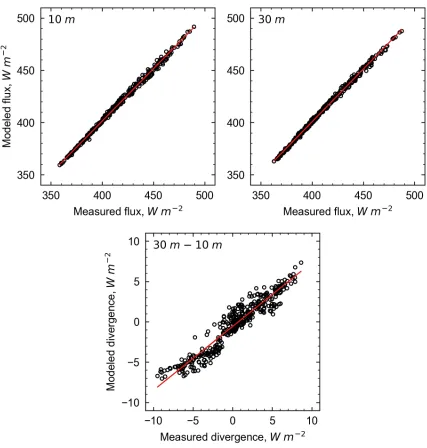
2.9 A comparison of 10m and 30 mmeasured and modeled longwave fluxes and

divergences - calculated as the difference between 30mand 10mfluxes - over

the 14 day evaluation period at Payerne, Switzerland. . . 42

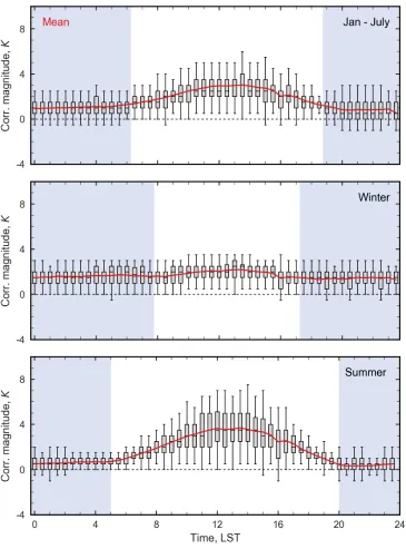
and Them, bfor the duration of the study period. Grey shading indicates nighttime.

The red line indicates mean correction magnitude at each time step. Box edges

represent the 25th and 75th percentiles with whiskers representing one standard

deviation. . . 45

2.11 Correction magnitude versus∆T_{hem, r - air}binned for season. . . 46

2.12 Correction magnitude versus∆Them, r - airbinned for clear and clouded days over

the summer months.. . . 47

2.13 Correction magnitude versus incoming shortwave and Them, r for the daytime

hours of the study period. . . 48

2.14 Correction magnitude versus Tairand water vapor content for the daytime hours

of the study period. . . 49

2.15 Hemispherical at-sensor atmospheric transmittance as a function of vapor

pres-sure for two pyrgeometer heights (10mand 30m) over a flat surface. Calculated

as the fraction of surface emission reaching the sensor height using MODTRAN

4.1 with Tsurf= Tair= 300Kwith water vapor as the sole atmospheric absorber. . 50

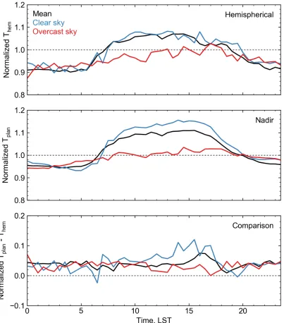
2.16 A comparison of mean normalized Them, r and Tplanat 30 minintervals over the

IOP. Shading indicates the area bounded by the first and third quartiles. n = 14 . . 51

2.17 Normalized Them, r, Tplan, and ∆Tplan - hem, r averaged over the IOP and for clear

sky and overcast case days. n = 14 . . . 52

2.18 Spectral dome transmittance for a Kipp & Zonen pyrgeometer overlaid with a

Planckian spectral radiance curve at T = 300 Kand the same curve shifted to

Actual sensor placement at the Sperrstrasse canyon is approximated by number 3. 61

2.20 Normalized wall, road, and roof view factors for nine sensor positions viewing

the simplified street canyon array from 2.17 times mean building height. Actual

normalized view factors refer to surface area proportions for the three facet types

in the Sperrstrasse street canyon. . . 62

2.21 Normalized wall, road, and roof view factors for nine sensor positions viewing

the simplified street canyon array from 3 times mean building height. Actual

normalized view factors refer to surface area proportions for the three facet types

in the Sperrstrasse street canyon. . . 63

2.22 Mean Them, r normalized against Tcomp for each sensor position over the 14-day

IOP for a sensor height of 2.17 times mean building height. Shaded area indicates

quartiles one through three. . . 65

2.23 Mean Them, r normalized against Tcomp for each sensor position over the 14-day

IOP for a sensor height of 3 times mean building height. Shaded area indicates

quartiles one through three. . . 66

2.24 Modeled Them, rversus Them, rderived via the parameterization scheme. . . 69

3.1 The EPiCC study site in Vancouver, Canada with urban and rural site locations

indicated. An image showing the approximate surface coverage at the urban

Sunset Tower site is shown in the inset (viewing towards the WSW from the top

of the tower). . . 88

at 30minintervals for the BUBBLE campaign. Results are interpolated between

months. . . 93

3.3 A heatmap of mean half hourly canopy layer UHI for each month calculated at

30min intervals for the BUBBLE campaign. Results are interpolated between

months. . . 94

3.4 A heatmap of the difference between mean half hourly hemispherical normalized

sUHI and canopy layer UHI for each month calculated at 30min intervals over

the BUBBLE campaign. Results are interpolated between months. . . 95

3.5 A heatmap of mean half hourly hemispherical sUHI for each month calculated

at 30 minintervals for a year-long subset of the EPiCC campaign. Results are

interpolated between months. . . 96

3.6 Hemispherical sUHI magnitudes for the eight month BUBBLE climatology (top)

and binned for December through February (middle) and April through July

(bot-tom) months. Grey shading indicates nighttime hours averaged over the bin

in-terval. . . 97

3.7 Hemispherical sUHI magnitudes for the year-long EPiCC climatology (top) and

binned for December through February (middle) and April through July (bottom)

seasons. Grey shading indicates nighttime hours averaged over the bin interval. . 98

3.8 A comparison of sUHI magnitudes from complete (sUHIcomp), hemispherical

(sUHIhem), and nadir (sUHInadir) remote sensed representations of the Sperrstrasse

canyon over the BUBBLE IOP. Each plot includes mean sUHI, as well as case

through July during the BUBBLE campaign versus integrated solar radiant

expo-sure meaexpo-sured at the Sperrstrasse site over the same 24hperiod. Color indicates

season: black is winter (Nov - Feb), white is spring (Mar - Apr), and red is

summer (May - Aug). . . 102

3.10 Maximum and mean 24 h hemispherical sUHI magnitude for each day of the

BUBBLE campaign versus mean wind velocity measured at approximately 2m

above ground at the Sperrstrasse site. Coloring indicates integrated solar radiant

exposure over each day. . . 103

3.11 Maximum and mean 24 hsUHI magnitude for each day of the BUBBLE

cam-paign versus atmospheric water vapor content measured at 2mat the Sperrstrasse

site. Similar patterns are observed when rural water vapor content is substituted.

Coloring indicates integrated solar radiant exposure over each day. . . 104

3.12 sUHI magnitude versus clUHI magnitude binned for day and night calculated

over the summer months of the BUBBLE campaign calculated for the Sperrstrasse

and Lange Erlen sites. Coloring in the daytime plot indicates time of day: Red is

morning (5:00 - 9:00 LST), gray is midday hours (9:30 - 17:00 LST), and yellow

is evening hours (17:30 - 20:00 LST). . . 105

3.13 Maximum and mean 24 h hemispherical sUHI magnitude for each day of the

EPiCC climatology versus integrated solar radiant exposure measured at the

Sun-set tower site over the same 24hperiod. Color indicates season: black is winter

(Nov - Feb), white is spring (Mar - Apr), red is summer (May - Aug), and blue

EPiCC climatology versus mean wind velocity measured at approximately 10m

above ground at the Sunset tower site. Similar patterns are observed when rural

mean wind velocity is substituted. Coloring indicates integrated solar radiant

exposure over each day. . . 108

3.15 Maximum and mean 24 h sUHIhemi magnitude versus mean atmospheric

wa-ter vapor content measured at 2mat the Sunset tower urban site in Vancouver,

Canada. Similar patterns are observed when rural water vapor content is

substi-tuted. Coloring indicates integrated solar radiant exposure over each day.. . . 109

3.16 sUHIhemi magnitude versus volumetric soil water content measured from 0.05m

below the surface at the Westham island site in Vancouver, Canada for May 2009

binned for day (11:00 - 17:00 LST) and night (22:00 - 5:00 LST) hours. . . 110

3.17 Top: Them from the Sperrstrasse urban and Lange Erlen and Village Neuf sites

and sUHI magnitudes calculated from the two rural stations for a representative

summer clear sky day. Middle and bottom: Mean normalized hemispherical

sUHI and Them, bcalculated for the Lange Erlen and Village Neuf sites. Data at

Village Neuf before noon were intermittent, thus n = 9 only applies to values

after 12:00 LST. Both sites are sampled over the same truncated period on days

with incomplete data. . . 112

3.18 Top: Mean Them, rfor the Sunset tower (urban) and Westham island (rural) sites

in Vancouver, Canada over May - Aug 2009. Middle: Mean heading/cooling

rates for urban and rural sites. Bottom: Mean sUHIhemiand aUHI and the hourly

rate of change in sUHIhemiand aUHI. n = 5905 . . . 117

Roman

Symbol Unit Property

C J m−3_s−1 _{heat capacity}

FOV deg sensor field of view

H m building height

H g m−3 _{water vapor mass density}

Kup W m−2 upwelling shortwave radiation

Kdown W m−2 downwelling shortwave radiation L0 W m−2 irradiance at the surface

Lz W m−2 irradiance at heightz

L↓_sky W m−2 _{upwelling longwave flux density emitted from the}

atmo-sphere

L↑_z W m−2 _{upwelling longwave flux density at heightz}

Lat_atm−sensor W m−2 _{the component of at-sensor irradiance from the atmosphere} Lat_surf−sensor W m−2 the component of at-sensor irradiance from the surface

Lat_total−sensor W m−2 _{total at-sensor irradiance}

Ldown W m−2 downwelling longwave flux density

Lup W m−2 upwelling longwave flux density

L0_z W m−2_sr−1 _{directional radiance through path lengthz}

P hPa atmospheric pressure

∆QA W m−2 net advective heat flux density

∆QG W m−2 net heat storage flux density

QE W m−2 latent heat flux density

QF W m−2 anthropogenic heat flux density

QH W m−2 sensible heat flux density

r - spectral sensor response

r - Planck weighted mean broadband sensor response

R W m−2_sr−1_µm−1 _{spectral directional radiance}

R↑₀ W m−2_sr−1_µm−1 _{upwelling spectral directional radiance at height zero} R↑_atm W m−2sr−1µm−1 upwelling spectral directional radiance emitted from the

at-mosphere

R↓_sky W m−2sr−1µm−1 downwelling spectral directional radiance emitted from the sky/atmosphere

R↑_z W m−2_sr−1_µm−1 _{upwelling spectral directional radiance at heightz}

t min time

T K temperature

Tadj K dome adjusted Them, r

Tair K air temperature

Tbias K bias in Them, rin terms of temperature

Tbright K surface brightness temperature

Tcalib K instrument calibration temperature

Tcomp K complete urban surface temperature

Temiss K emission temperature

Them K urban surface temperature viewed from a hemispherical

re-mote sensor

Them, b K urban surface brightness temperature viewed from a

hemi-spherical remote sensor

Them, r K urban surface radiometric temperature viewed from a

hemi-spherical remote sensor

plan

Trad K radiometric surface temperature

Troad K road surface temperature

Troof K roof surface temperature

Tsurf K surface temperature

Twall K wall surface temperature

aUHI K air temperature urban heat island magnitude

clUHI K canopy layer air temperature urban heat island magnitude sUHI K surface temperature urban heat island magnitude

sUHIcomp K surface urban heat island magnitude calculated from Tcomp

sUHIhem K surface urban heat island magnitude calculated from Them, r

sUHIplan K surface urban heat island magnitude calculated from Tplan VB - effects from background climate on observation of a given

meteorological variable

VH - effects from the urban environment on observation of a

given meteorological variable

VL - effects from local topography on observation of a given

me-teorological variable

VM - observed meteorological variable

VM,U - observed meteorological variable (urban)

VM R - observed meteorological variable (rural)

W m building width WD deg wind direction WV m s−1 _{wind velocity}

z m height or path length

zH m mean building height

zt m layer thickness

α - albedo

- emissivity

λ - spectral emissivity

θ deg zenith angle

λ µm wavelength

λB - plan area of buildings

λC - complete aspect ratio

λI - plan area of impervious ground

λP - plan aspect ratio

λT - plan area of trees

λV - plan area of ground vegetation

ν cm−1 wavenumber

σ Wm−2_K−4 _{Stefan Boltzmann constant}

σH m standard deviation of building height

τ - atmospheric transmittance

τd - atmospheric transmittance

τλ - spectral atmospheric transmittance

τΦ - hemispherical atmospheric transmittance φ deg azimuth angle

Φ - view factor

Chapter 1

Introduction

Urban development drastically changes the character of the surface. Replacement of natural terrain with roads, buildings, parks, and other urban features modifies the geometry of the surface as well as its thermal, radiative, moisture, and aerodynamic properties. These modifications, combined with anthropogenic emissions of heat, result in a distinct urban climate; one which is often warmer, a phenomenon termed the urban heat island effect (UHI). As both the Earth’s population and the urbanized fraction of that population increase (United Nations,2014), cities grow and more people are exposed to urban-modified atmospheres. Thus, understanding how cities interact with the climate across spatiotemporal scales has important implications for human health, energy efficiency, and for informing future urban development. This, in part, has prompted significant expansion in study of the urban effect on climates, with particular focus on characterization of the urban effect on surface (Tsurf) and air (Tair)

The temperature of a surface (urban or otherwise) at its interface with the atmosphere is defined as the net result of the surface energy balance (Oke et al.,2017), wherein change in temperature at timetfor a surface with thicknessztand heat capacityCcan be solved as,

C ∂Tsurf

∂t zt=Q ∗

+QF −QH −QE −∆QA−∆QG (1.1)

whereQ∗is net radiation at the surface,QF,QH, andQE are fluxes of anthropogenic, sensible,

and latent heat respectively,∆QAis net advection of surface heat to or from the volume of air

above the surface, and∆QGis net storage of heat by the substrate below. A change in Tsurfis

translated to change in Tairas the surface exchanges energy with the atmosphere above it,

primarily via convection and radiation. As such, Tsurfand Tairare inextricably linked,

particularly near to the ground, and a city’s altered surface characteristics and energy balance manifest in modifications to both surface and air temperature regimes.

The notion that urban modifications to the environment produce elevated Tairand Tsurfis

not new, with the first formal studies of the urban effect on Tairdating back toHoward(1833)’s

identification of ”artificial warming” and ”urban contamination” in his characterization of spatial patterns of Tairin early 19th century London, England. Conceptually, contemporary

studies of urban climate do not stray far fromHoward(1833), by seeking to isolate and quantify the urban signal in measured or modeled assessment of a given meteorological variable.

control have shown promise (Krayenhoff et al.,2014;Gastellu-Etchegorry et al.,1996;Masson,

2000;Martilli et al.,2002) yet the inherent complexity in simulating flows of energy,

momentum, and mass at the scales necessary to represent the full range of physical processes over realistic environments remains an on-going challenge. Thus, accurate assessment of how a city affects the climate is a deceptively challenging task. To address this,Lowry(1977) presents a framework to isolate the urban effect in observation of a given meteorological variable. In his framework - termed the ”Lowry method” - measurement of a meteorological variable (VM) is

the sum of forcings from the background climate and synoptic conditions (VB), local

topography (VL), and the urban landscape (VH)

VM =VB+VL+VH (1.2)

Thus, isolation of the urban effect on observedVM simply requires the removal ofVB

andVL. This can be achieved by subtracting some urban affected observation (VM, U) from a

non-urban observation (VM, R) whereVH, R= 0,

VM,U −VM,R = (VB+VL+VH)−(VB+VL) =VH (1.3)

simplified as,

VH =VM, U −VM, R (1.4)

Study of the UHI with respect to Tsurf(sUHI) and Tair(aUHI) - typically referring to Tair

measured from approximately 2mabove ground level, yielding a ”canopy layer” UHI (clUHI) -tacitly falls into such a framework, by replacingVM, U −VM, Rwith∆TU - R. However, in spite

observational aUHI studies suggests that that simplicity may not translate well to real world analysis. In a points based assessment of 190 aUHI studies published between 1950 and 2007,

Stewart(2011) found that nearly 50% of studies are ”scientifically indefensible”. In the analysis, each study was given a ”passing” or ”failing” grade and ranked based on

methodological quality in the following criteria: conceptual model, operational definitions, instrument specification, site metadata, site representativeness, number of replicates, weather control, surface control, and synchronisity. Of the 190 surveyed studies, only 13% were derived from field sites that were sufficiently representative of the local-scale environment or lacked the meta-data to make such a determination. 89% lacked meta-data altogether. These findings suggest a significant gap between conceptual simplicity and practical realities in UHI analysis.

Conceptual problems in the aUHI literature are particularly discouraging as they are not the result of an evolution in measurement techniques or improved instrumentation. Techniques to observe and analyze aUHI did not see significant evolution or improvement in the period between 1950 and 2007 - in fact,Stewart(2011) suggests the opposite: a disproportionately large number of studies deemed scientifically sound were published early in the study purview. In the five years since its publication, aUHI study has seen further expansion and, as such, it is difficult to assess whether its critical analysis has prompted a shift towards more thoughtful, careful, and methodical study of aUHI, notwithstanding its relevance in study of the urban effect on other meteorological variables. Thus, in study of the urban effect on variables for which significant methodological shifts have or will occur, the warnings implicit inStewart

(2011) are particularly salient, as difficulties found in translating ”Lowry”-esque conceptual models to real world observations may be compounded by significant changes in methodology. What is clear in light of these findings, however, is that assessment of the urban effect on climate isfundamentally difficultin spite of its conceptual simplicity.

undergone significant recent evolution and methodological problems arise in large part from conceptual shortcomings and simple carelessness, study of the urban effect on land Tsurfis

relatively new and significantly more complex. As such, methodological problems in sUHI study can arise from both conceptual flawsandinstrument biases. In spite of these difficulties, the introduction of new methods, instruments, and analytical techniques in remote sensing of upwelling thermal infrared (TIR) radiation has lead to a rapid proliferation of study of urban Tsurfand the sUHI - much of which is focused on remote sensing of TIR radiation. In the

decades preceding this thesis, a combination of factors has lead to an increased focus on remote sensed study of urban Tsurf:

• The proliferation of satellite and aerial TIR radiation remote sensors and ”openness” in data access policies.

• Improvements in sensor spatial, spectral, and radiometric resolutions.

• An increased focus on the importance of the surface in both determining and understanding key near-ground micro-meteorological phenomena.

• Interest in urban Tsurffor human thermal comfort, energy conservation, and sUHI

mitigation applications.

Remote sensed study of the urban effect on land Tsurfhas been critical in characterizing

large-scale spatial and temporal patterns of sUHI (Peng et al.,2012;Streutker,2003;Imhoff et al.,2010). However, the methodological and conceptual concerns raised inStewart(2011) in combination with the wide (and broadening) range of methodologies for remote sensed urban Tsurfretrieval should prompt critical assessment of the remote sensed sUHI literature. At the

available, and questions raised in critical assessments of remote sensed urban TsurfinRoth et al.

(1989) andVoogt and Oke(2003) have gone largely unaddressed. An increasingly dogmatic focus on improving spatial and radiometric resolutions has left other biases in remote sensing of urban environments largely ignored in sUHI literature. This suggests that similar conclusions to those found of aUHI literature inStewart(2011) are possible (if not likely) for study of sUHI. Assessment of these biases is, therefore, paramount to ensure assessments of the urban effect on Tsurfare robust, methodologically valid, and comparable across techniques, space, and time.

1.1

Biases and shortcomings in thermal remote sensing of

urban T

Traditional methods for urban Tsurfmeasurement are subject to a suite of geometric and

temporal biases. Geometric biases are the result of urban modification of surface structure and thermal and radiative properties combined with the narrow field-of-view (FOV) viewing geometry of conventional remote sensors:

Undersampling of surface 3-dimensionality by narrow-FOV remote sensors

surface from an oblique angle sees some array of walls, rooftops, and roads depending on its orientation. For a sensor in the nadir, increasing FOV introduces sampling of vertical features. To illustrate how sensor-surface geometry influences sampling of the urban surface by narrow-and wide-FOV sensors, Figure1.1shows FOVs for the three sensor orientation/type

combinations.The vast majority of urban thermal remote sensing is done via a narrow-FOV sensor viewing from the nadir.

Figure 1.1: Projected FOVs for a narrow-FOV sensor at nadir and oblique angles, and a wide-FOV hemispherical sensor viewing an idealized urban array with building widthW, height 2W, and inter element spacingW. Figure from Adderley et al. (2015) under a Creative Commons Attribution 4.0 License.

Directional dependence in remote sensed urban T

In addition to modifying how a remote sensor samples the surface, the convoluted 3-dimensional structure of the urban surface modifies the surface radiation budget, resulting in strong micro-scale spatiotemporal contrasts in urban Tsurf, which depend on surface-sun

geometry. These microscale variations in urban Tsurfare often amplified by significant geometric

sensor with some inherent geometric bias, urban Tsurfis directionally dependent - constituting

an ”effective anisotropy” of urban Tsurf, shown in Figure1.2. The qualifier ”effective” is used to

differentiate directional contrasts in urban Tsurfthat arise from a city’s 3-dimensional surface

structure from those resulting from the non-Lambertian nature of individual urban facets (e.g. walls, rooftops, or roads). The magnitude of urban effective anisotropy can reach up to 10 to 12

Kand is highly dependent on surface-sensor-sun geometry, surface structure, and urban materials (Krayenhoff and Voogt,2016;Voogt and Oke,1997;Lagouarde et al.,2012).

Figure 1.2: A narrow-FOV sensor viewing an idealized urban surface from two angles. Left: viewing the surface approximately perpendicular to the sun’s angle. Right: viewing the surface approximately parallel to the sun’s angle. The two viewing angles yield different remote sensed Tsurfby sampling different arrangements of sunlit and shaded features. Both will deviate from an

area weighted ”complete” urban Tsurf.

Geometric undersampling by narrow-FOV remote sensors results in differences in remote sensed urban Tsurfbased on a sensor’s viewing direction and the assemblage of facets

temperature - often calculated as an area weighted average of wall, rooftop, and road Tsurf- by

differentially biasing sunlit or shaded facets. Similarly, a sensor in the nadir will tend to

overestimate daytime urban Tsurfand underestimate nighttime Tsurf, from a bias towards rooftop

facets that are differentially hot by day and cool by night and a neglect of wall facets which are differentially cooler by day and warmer by night. As the effect of geometric biases is highly dependent on surface-sensor-sun geometry and requires significant instrumentation for observation, its influence in the remote sensed sUHI record is presently unknown.

Temporal biases in thermal remote sensing of urban areas occur across multiple time scales including the following:

Contamination by turbulence forced, high frequency fluctuations in urban T

Using time-sequential thermographyChristen et al.(2012) found that many common urban fabric types (e.g. rooftops, walls, roads, and vegetation) display large micro-scale (second to minute) fluctuations in Tsurf. The magnitude of these is inversely related to surface thermal

admittance and is currently, poorly understood. Most thermal remote sensors provide

instantaneous, rather than temporally averaged, Tsurfand thus are subject to contamination by

high-frequency fluctuations. These biases are difficult to estimate in urban environments, where a large variety of fabric materials can produce significant geometric and spatial contrasts in thermal admittance — and thus directional and spatial variations in the magnitude of microscale fluctuations depending on the facet material types viewed by the sensor.

Discontinuity in satellite overpass cycles.

resolution for a daily repeat cycle - as is the case with MODIS - or sacrifices temporal resolution for a higher spatial resolution - ASTER or Landsat. These satellites cannot be used to assess the temporal development of sUHI without significant interpolation. Work inFreitas et al.(2013),

Zakˇsek and Oˇstir(2012), andWeng and Fu(2014) used thermal images from geostationary satellite remote sensors to overcome this limitation, but a coarse spatial resolution limits the applicability of these methods in complex heterogeneous urban areas, especially at mid to high latitudes. Similar work inHuang et al.(2016) andZhou et al.(2013) used an annual temperature cycle and diurnal temperature cycle genetic algorithm respectively to interpolate climatologies of urban Tsurfand sUHI from discontinuous data. However, the diurnal and seasonal urban Tsurf

cycles presented in these studies are only applicable under ”ideal” cloudless conditions and are specific to test cities. In general, studies that address temporal discontinuities in the urban Tsurf

record are not the norm and the vast majority of sUHI study remains temporally sparse.

Clear-sky bias

Clouds absorb TIR radiation. Thus, satellite remote sensing of TIR radiation emitted by the surface requires clear sky conditions. Although the urban effect on Tsurfis most evident

under ”satellite friendly” clear sky conditions (manifesting as large sUHI magnitudes), a clear sky bias likely entails overestimation of ”all-sky” sUHI and further adds to discontinuities in the remote sensed urban Tsurfrecord.

As is the case with geometric biases, the magnitude of these temporal biases in remote sensed urban Tsurfis difficult to quantify without long-term ground truthing campaigns or

1.2

Research questions and objectives

Prompted by these shortcomings in the remote sensed urban Tsurfrecord, and in an effort

to better understand the temporal and geometric aspects of sUHI, this thesis introduces a method to provide hemispherical, temporally continuous urban Tsurffor sUHI analysis to

address the following questions:

1. What is the nature of urban surface temperature when viewed from a hemispherical downward-facing radiometer? And how does it relate to urban temperatures derived from other methods for urban surface temperature retrieval?

2. What is the diurnal and seasonal nature of the surface urban heat island effect? In an attempt to answer these questions, this thesis

• Develops and evaluates a method to retrieve atmospherically corrected hemispherical radiometric urban surface temperatures from time-continuous measurements of upwelling longwave radiation.

• Compares urban surface temperatures and surface urban heat island magnitudes retrieved using the method to common remote sensed representations of the urban surface.

• Derives two long term climatologies of hemispherical urban surface temperatures to observe seasonal and diurnal patterns of the surface urban heat island effect in Basel, Switzerland and Vancouver, Canada.

References

Christen, A., Meier, F., and Scherer, D. (2012). High-frequency fluctuations of surface temperatures in an urban environment. Theoretical and Applied Climatology, 108(1-2):301–324.

Freitas, S. C., Trigo, I. F., Macedo, J., Barroso, C., Silva, R., and Perdig˜ao, R. (2013). Land surface temperature from multiple geostationary satellites. International Journal of Remote

Sensing, 34(9-10):3051–3068.

Gastellu-Etchegorry, J. P., Demarez, V., Pinel, V., and Zagolski, F. (1996). Modeling radiative transfer in heterogeneous 3-D vegetation canopies. Remote Sensing of Environment,

58(November 1995):131–156.

Howard, L. (1833). The climate of London, volume 1 - 3. Harvey and Dorton, London. Huang, F., Zhan, W., Voogt, J., Hu, L., Wang, Z., Quan, J., Ju, W., and Guo, Z. (2016).

Temporal upscaling of surface urban heat island by incorporating an annual temperature cycle model: A tale of two cities. Remote Sensing of Environment, 186:1–12.

Krayenhoff, E. S., Christen, A., Martilli, A., and Oke, T. R. (2014). A Multi-layer Radiation Model for Urban Neighbourhoods with Trees. Boundary-Layer Meteorology,

151(1):139–178.

Krayenhoff, E. S. and Voogt, J. A. (2016). Daytime thermal anisotropy of urban neighbourhoods: Morphological causation. Remote Sensing, 8(2):1–22.

Lagouarde, J. P., H´enon, A., Irvine, M., Voogt, J., Pigeon, G., Moreau, P., Masson, V., and Mestayer, P. (2012). Experimental characterization and modelling of the nighttime

directional anisotropy of thermal infrared measurements over an urban area: Case study of Toulouse (France). Remote Sensing of Environment, 117:19–33.

Lowry, W. P. (1977). Empirical estimation of urban effects on climate: a problem analysis.

Journal of Applied Meteorology, 16:129–135.

Martilli, A., Clappier, A., and Rotach, M. W. (2002). An urban surface exchange parameterization for mesoscale models. Boundary-Layer Meteorology, 104:261–304. Masson, V. (2000). A physically-based scheme for the urban energy budget in atmospheric

models. Boundary-Layer Meteorology, 94(3):357–397.

Oke, T. R., Mills, G., Christen, A., and Voogt, J. A. (2017). Urban Climates. Cambridge University Press.

Peng, S., Piao, S., Ciais, P., Friedlingstein, P., Ottle, C., Br´eon, F. M., Nan, H., Zhou, L., and Myneni, R. B. (2012). Surface urban heat island across 419 global big cities. Environmental

Science and Technology, 46(2):696–703.

coastal cities and the utilization of such data in urban climatology. International Journal of

Remote Sensing, 10(11):1699–1720.

Stewart, I. D. (2011). A systematic review and scientific critique of methodology in modern urban heat island literature. International Journal of Climatology, 31(2):200–217.

Streutker, D. (2003). Satellite-measured growth of the urban heat island of Houston, Texas.

Remote Sensing of Environment, 85(3):282–289.

United Nations (2014). World Urbanization Prospects: The 2014 Revision. Technical report, Department of Economic and Social Affairs.

Voogt, J. A. and Oke, T. R. (1997). Complete urban surface temperatures. Journal of Applied

Meteorology, 36(9):1117–1132.

Voogt, J. A. and Oke, T. R. (2003). Thermal remote sensing of urban climates. Remote Sensing

of Environment, 86(3):370–384.

Weng, Q. and Fu, P. (2014). Modeling diurnal land temperature cycles over Los Angeles using downscaled GOES imagery. ISPRS Journal of Photogrammetry and Remote Sensing, 97:78–88.

Zakˇsek, K. and Oˇstir, K. (2012). Downscaling land surface temperature for urban heat island diurnal cycle analysis. Remote Sensing of Environment, 117:114–124.

Chapter 2

An atmospheric correction method to

derive hemispherical time-continuous

urban surface temperature

2.1

Introduction

TIR remote sensing of land surface temperature has emerged as a primary research focus in climatology, as researchers seek to better describe spatiotemporal patterns of Tsurfglobally

and better understand how anthropogenic modification of the Earth’s surface influences land Tsurfand impacts climate at various scales. Over the last two decades, application of thermal

Within urban climatology, a combination of satellite, aerial, and ground-based thermal remote sensors have been integral in elucidating the spatial (Roth et al.,1989), temporal (Peng et al.,2012), and geometric (Voogt and Oke,1997) effects of the built environment on land Tsurf; in evaluating and partitioning urban surface energy balances (Bastiaanssen W. G. M. et al.,

1998;Yamaguchi and Kato,2005;Frey et al.,2007) and; in characterizations of the relationship between surface and boundary-layer air temperatures (Tair) (Stoll and Brazel,1992). These

advances have been aided by substantial improvements in sensor spatial, spectral, and radiometric resolutions, and by the proliferation of both large-scale public satellite remote sensing campaigns and low-cost aerial and near-ground thermography. However, in spite of its widespread usage, several questions concerning the use and validity of urban remote thermal remote sensing, first posed inRoth et al.(1989), have yet to be sufficiently answered, viz,

1. What is the nature of the surface ’seen’ by a thermal remote sensor?

2. How does Tsurfobserved by a remote sensor relate to the ’true’ temperature governing the

surface-atmosphere interface?

In this paper, we seek to examine question two by introducing and evaluating a method for atmospheric correction of near-ground hemispherical TIR radiation - measured via pyrgeometer - for hemispherical radiometric temperature (Them, r) retrieval. These measures are common to

most urban energy balance assessments because they are made as a part of the net radiation measurement and thus constitute a hitherto untapped method for urban Tsurfanalysis. A

companion paper responds to question one through an analysis of two long term climatologies of Them, rand derived surface UHI magnitudes (sUHI), to quantify geometric and temporal

2.2

Atmospheric effects on TIR radiation

Although most thermal remote sensors operate within one of the atmospheric windows -where atmospheric effects are minimal - virtually any remote sensed TIR signal is subject to radiative effects from the layer of atmosphere between the surface and the sensor. Over much of the thermal infrared waveband the atmosphere emits radiation and absorbs a fraction of

radiation emitted by the surface. Thus, a remote sensed TIR signal is almost certainly not equal to the ground emitted signal. Spectral radiance received by a sensor at height (z) can be

described by a function deviating from a Planck curve at Tsurfbased on the spectral

transmittance of the intervening atmosphere, with the magnitude of that deviation determined by the difference between Planck curves calculated from Tsurfand ambient Tair. A radiative transfer

Figure 2.1: At-sensor spectral directional radiances computed in MODTRAN 4.1 (Berk et al., 1987) for short (30m) and long (3000m) path lengths (z) with Planck curves indicating spectral radiances at Tsurf= 300Kand Tair= 290K.

Atmospheric effects can lead to differences between the ’true’ radiometric Tsurfand the

remote sensed Tsurfof over 10Kfor satellite platforms (Cooper and Asrar,1989) and over 6K

for near-ground sensors (Meier et al.,2011). Moreover, because atmospheric effects are a function of non-uniform and spatiotemporally variant surface and atmospheric properties, their associated errors change depending on instrument type, surface-sensor geometry, study

of most thermal remote sensed studies (urban or otherwise) these effects cannot be ignored. Spectral transmission of longwave radiation through a given layer of atmosphere is dependent on total column absorber content (the principal broadband TIR absorbers are H2O,

CO2, and to a lesser extent O3, N2O, CO, CH4, and O2(Miskolczi and Guzzi,1993)). Holding

Figure 2.2: Spectral transmission of water vapor as a function of height. Model results from MODTRAN 4.1 for radiance emitted from a planar surface at 300Kthrough an atmosphere with water vapor content of 8g m−3. Sampled at heights of 1, 5, 10, 15, 20, 25, and 30m.

2.2.1

Describing radiation as received by a remote sensor

R↑_z(λ, θ, φ) = τλλR

↑

0(λ) + (1−λ)R

↓

sky(λ) + (1−τλ)R

↑

atm(λ) (2.1)

whereλ is spectral surface emissivity,τλ is spectral ”slab” transmittance through the layer

between the emitting surface(z = 0)andz. Directional radiances upwelling from the atmosphereR↑_atm, and the surfaceR↑₀, and downwelling from the skyR↓_sky, can be described spectrally or integrated over a waveband bounded byλ1andλ2as Planck’s law

R(θ, φ) =

Z

λ1

R(λ, θ, φ)dλ= λC1

πλ5  exp   C2 λT     (2.2) where C1=3.7404·108W µ4m−2, C2 =14387µK, andT is emitter temperature.

Measured by a narrow-FOV sensor mounted at heightz,R↑_z(λ, θ, φ)passes through an instrument filter (or dome) with spectral transmittanceτd, and is integrated over the sensor

waveband to yield adirectional radianceL0_zas ’seen’ by the sensor

L0_z(θ, φ) =

Z λ2

λ1

τd(λ)R↑z(λ)dλ (2.3)

which, integrated over the hemisphere with respect to zenithθangle and azimuthφangle, yields

anirradianceLat heightz,

Lz =

Z 2π

0

Z π/2

0

2.2.2

Relating TIR and surface temperature

TIR radiation received by a remote sensor can be related to a surface temperature in a number of ways — each producing different conceptions of Tsurffrom different instrument and

sensor types. As such, the term ”surface temperature” with respect to a remote sensed TIR radiation is vague and can refer to several definitions of ”surface” and ”temperature”. Thus, proper terminology must be attached to land Tsurfinferred from TIR radiation. Definitions and

nomenclature conventions for multiple methods for Tsurfretrieval are discussed at length in

Norman and Becker(1995).

IrradianceLz received by a broadband hemispherical sensor (such as a pyrgeometer), can

be used to infer ahemispherical brightness temperatureThem, bthrough an inversion of the

Stefan-Boltzmann law,

Them, b =

4

r

Lz

σ (2.5)

whereσis the Stefan-Boltzmann constant.

Adirectional brightness temperatureTbright(θ, φ)from some viewing angle described by

θandφcan be inferred from directional radiance via equation2.5by replacingLzwithL0z

multiplied by a coefficient. This method is commonly used to infer Tbright(θ, φ)from infrared

thermometers (IRT) operating over the atmospheric window - where atmospheric effects are minimal and Tbrightis a reasonably accurate approximation of Tsurf. However, constants must be

calibrated for the range of expected Tsurfas the relationship betweenLz andL0z is not perfectly

linear with respect to emitter temperature.

Inversions of uncorrectedLzorL0zyield a temperature equal to that of a blackbody

toL0and, by extension,L0z is unlikely to be equal toL00, Them, batz = 0and Them, batz often

show significant deviation. Hence, Tbrightand Them, bare generally considered only a rough

approximation representation of radiometric Tsurf.

To retrieve a more accurate estimation of the ’true’ Tsurf, the same inversions can be

applied to TIR measurements after correction for atmospheric effects (e.g. modification of the remote sensed TIR signal to represent the same signal atz = 0emitted from a homogeneous, isothermal, blackbody emitter) to yield adirectional radiometric surface temperatureTradfrom

atmospheric corrected directional radiances and ahemispherical radiometric surface

temperatureThem, rfrom atmospherically corrected irradiances. Tradand Them, rprovide a better

approximation of the true Tsurfby representing the temperature at which emitting surfaces are

radiating, integrated over the sensor FOV.

2.2.3

Atmospheric correction of near-ground TIR radiation

A large number of correction routines have been developed to remove atmospheric and emissivity effects from aerial and satellite TIR signals and derive accurate Trad. Methods range

from simple mono-window (Qin et al.,2001) and split-window (Wan and Dozier,1996) routines for single-channel and multi-channel remote sensors, to schemes that integrate a radiative transfer code to isolate the surface emitted signal from interfering signals. Boundary conditions are standard across most correction methods: generally requiring vertical profiles of Tair, humidity, pressure, and aerosol content to remove atmospheric effects, and surface

wide-field-of-view (FOV) radiometer mounted to view rough terrain.

Atmospheric correction of near-ground remote sensed TIR radiation is subject to a unique set of challenges compared to traditional satellite and aerial platforms. Wide-FOV remote sensors have complex, multiple line-of-sight (LOS) path length geometries - illustrated in Figure2.3for a downward facing pyrgeometer. Surface-sensor geometry varies significantly over the sensor FOV as some path lengths intersect with raised vertical, sloped, and horizontal features. This creates the potential for non-uniform atmospheric effects over the sensor FOV and necessitates a multi-LOS correction to retrieve accurate Them, r. In effect, with near-ground

wide-FOV sensors, surface geometry is non-trivial and must be represented in atmospheric correction routines. In contrast, over a scene retrieved via satellite, spatial viability in surface geometry and LOS angle have a negligible effect on path length. Atmospheric correction routines for satellite retrieved TIR radiation, therefore, assume uniform or single-LOS geometry because the TIR signal passes through a relatively constant volume of atmosphere over the projected sensor FOV, regardless of surface geometry.

Several multi-LOS correction routines have been developed to remove atmospheric effects on near-ground remote sensed TIR radiation:Meier et al.(2011) describes a correction method for oblique angled thermal imagery of urban terrain. In the method, spatially distributed LOS geometries were calculated by linking each image pixel to the corresponding 3-d

coordinates of its viewpoint on a digital building model (DBM). Path lengths were then calculated as the distance between each pixel’s corresponding location on the DBM and the sensor represented as the vanishing point of a 3-dimensional pyramidic projection from the sensor’s location in the DBM. A pixel-by-pixel correction was then applied to remove

atmospheric effects and retrieve Trad for each pixel at 30 minute intervals, resulting in a brief,

time-continuous climatology of urban Trad. However, the method uses thermal images in

conjunction with a DBM to calculate path length geometries for each pixel’s LOS - a technique not possible with a pyrgeometer, which returns a single integrated value over the sensor FOV. Moreover, the target instrument operates over a narrow waveband with relatively uniform spectral sensor response, reducing the magnitude and variance in atmospheric transmission over the sensor response curve. Thus, the method is not directly generalizable to correct TIR

radiation measured via pyrgeometer.

Kotani and Sugita(2009) describes a method for correction of wide-FOV (pyrgeometer) TIR irradiances over a homogeneous planar surface. In this method, path lengths were

calculated for six sensor heights. Radiances were then modeled using the LOWTRAN (Kneizys et al.,1988) radiative transfer code initialized at5◦ intervals and integrated over the hemisphere to retrieve irradiances for a suite of Tsurf, and ambient Tairand humidities. The resulting lookup

table (LUT) of values is then used to correctLz and quantify atmospheric effects on remote

sensedLzmeasured from several sensor heights.

measured via downward facing pyrgeometer a method which combinesMeier et al.(2011)’s representation of complex surface geometry andKotani and Sugita(2009)’s broadband hemispherical integration is needed.

2.3

A ”rolling lookup table” method for hemispherical

atmospheric correction

The ”rolling lookup-table” method described in this study uses a sensor view model in conjunction with a radiative transfer code to model hemispherical irradiances upwelling from a simplified isothermal 3-dimensional representation of the urban surface. In summary, the method (depicted in Figure2.4) uses vertical profiles of measured Tairand humidity to model

at-sensor spectral radiances at 5◦increments over the sensor FOV for a predetermined range of possible Them, rat each time-step. Spectral directional radiances are convolved by a dome

transmittance curve, integrated over the sensor waveband, and weighted for their respective angular view factor. Weighted directional radiances are then integrated over the hemisphere and aggregated into a LUT of modeled irradiance - Them, rpairings for each time step, unique to the

vertical profile of measured Tairand humidity. Finally, for each time step, measured irradiances

are matched with the closest modeled irradiances in the LUT to return an atmospherically corrected radiometric hemispherical surface temperature. This process is repeated at 30 minute intervals to yield a continuous climatology of urban Them, r. The following sections introduce the

Figure 2.4: A workflow schematic depicting the input, model, and output-processing steps of a ”rolling lookup table method” for hemispherical radiometric surface temperature retrial.

2.3.1

Study area

As discussed in section2.2.3, atmospheric correction of longwave irradiances measured from downward-facing, near-ground, wide-FOV sensors must account for complex surface geometry. Thus, routines to retrieve atmospherically corrected urban Them, rfrom upwelling

longwave irradiances are inherently site specific. However, it is important to note that although correctionmagnitudesdescribed in this paper are not necessarily generalizable, the correction

methoddescribed in this paper can readily be adapted to different study sites, sensor types, and

unique surface geometries.

With methodological generalizability in mind, a ”rolling lookup table” atmospheric correction method was developed to retrieve radiometric Them, rfor a climatology of upwelling

longwave irradiances measured from above the Sperrstrasse street canyon in Basel, Switzerland. The site, instrumented as a part of the Basel Urban Boundary Layer Experiment (BUBBLE)

representative of local climate zone (LCZ) 21 _{Stewart and Oke(2012). LCZ classification was}

based on an assessment of surface characteristics in a 250mcircular area extending from the Sperrstrasse tower using a 1mraster digital building model (DBM). Thus, the morphological parameters identified inRotach et al.(2005) are representative of a majority of the pyrgeometer footprint. Vegetation was not included in the DBM, and is not represented in morphological assessment or the sensor view model, however, the street canyon and surrounding area has little vegetation. The location of the Sperrstrasse urban site and the two rural reference sites used in sUHI analysis are included in Figure2.5.

1_{Site surroundings can be described by the following morphological parameters: mean building height: 14.6m,}

For the eight month period between December 2001 and July 2002 of the BUBBLE campaign, a triangular lattice tower was installed within the Sperrstrasse street canyon. Its location was offset towards the southeast facing wall near the along-canyon center of the

canyon. Instruments to observe a full suite of meteorological variables and fluxes of heat, mass, and momentum were mounted at various levels on the tower. Profiles of Tairand humidity were

measured at seven heights extending from 2.5mto 31.5mabove the canyon floor (with the highest observation level at approximately 2.17 times mean roof level). Upwelling and

downwelling short/longwave fluxes were obtained from radiometers mounted at the lowest and highest measurement levels, with an additional downward facing pyrgeometer mounted at roof level near the center of the street canyon. In addition, during a month-long summertime intensive observation period (IOP) an array of narrow-FOV IRTs was installed to sample representative individual facet surface temperatures (Tfacet). A schematic of the locations of

IRTs and pyrgeometers within the Sperrstrasse canyon is included in Figure2.6. A subset of the BUBBLE dataset is available at

The BUBBLE Sperrstrasse site was chosen here for two primary reasons: 1. The site provided a long-term climatology of radiation and meteorological variables for a representative mid-latitude city. This allowed for examination of urban Tsurf, sUHI, and atmospheric correction

magnitudes over a wide range of representative mid-latitude conditions. 2. Inclusion of Tfacet

over the IOP allows for investigation of the effect of sensor FOV and viewing direction on remote sensed urban Tsurffor common methods for urban Tsurfretrieval. This directional

dependence of urban Tsurf- termed ”effective anisotropy” - refers to the notion that a remote

sensed TIR signal can vary based on the combined effects of surface-sensor-sun geometry and the convoluted, 3-dimensional structure of the urban surfaceVoogt and Oke(1998).

Facet surface temperatures measured during the summertime IOP allow for direct climatological comparison of Them, rto common remote sensed representations of the urban

surface calculated from weighted averages of wall (Twall), road (Troad), and roof (Troof)

temperatures. Plan and complete aspect ratios are used to derive weightings for nadir remote sensed (Tplan) and complete (Tcomp) representations of urban surface temperature - described in

Table2.1. Tcomprepresents a complete urban Tsurf, where facet temperatures are averaged based

on their proportion of the complete urban surface area, while Tplanrepresents the Sperrstrasse

site as viewed by a narrow-FOV remote sensor in the nadir. To facilitate comparison over the IOP, Them, rand Tplanwere divided by Tcompand averaged at each time step over the IOP to yield

normalized mean Them, rand Tplanat 30-minute intervals. Through comparison of Them, rto Tplan

and Tcompwe investigate the effect of sensor-surface geometry on remote sensed urban Tsurfand

Table 2.1: Weights applied to individual facet temperature components in to calculate complete and nadir temperatures for the Basel Sperrstrasse street canyon.

Road Northwest Southeast Northwest Southeast Roof Roof Wall Wall Complete (Tcomp) 0.33 0.16 0.16 0.16 0.16

Nadir (Tplan) 0.46 0.27 0.27 0.00 0.00

2.3.2

Modeling path lengths of 3-dimensional terrain

The sheer number of unique path length geometries inherent with wide-FOV radiometry of urban areas makes full 3-dimensional radiative transfer simulation difficult and

computationally intensive - particularly when correcting a long-term climatology of irradiances or Them, r. In this method, to improve efficiency, radiances are calculated for azimuthally

averaged path lengths that represent average surface-sensor geometry for each solid angle ”slice” of the sensor FOV. Thus, hemispherical radiative transfer is reduced to a 2-dimensional problem similar to that shown in Figure2.7. This greatly reduces the computational time required to model each irradiance - Them, rpairing, as angular radiances can be computed as a

function of zenith angle alone and subsequently weighted and integrated 3-dimensionally over the hemisphere.

To calculate surface-sensor geometries, the Surface-Sensor-Sun Urban Model (SUM) (Soux et al.,2004) is initialized with a simplified, orthogonal 3-dimensional DBM that represents surface geometry of the surrounding area. SUM uses a four-dimensional array to represent surface morphology with three spatial dimensions (x,y, andz), withzrepresenting height above thex,yplane. An additional fourth dimension is used to store information

sensor and calculates distance from ”seen” patches to the sensor. Path lengths are binned at 5◦ increments of zenith angle and averaged to return an azimuthally-independent mean path length for each bin. In addition, while retrieving path length geometries, SUM calculates view factors for each solid angle ”slice”, which are later used to weight angular radiances in the

hemispherical integration post-processing steps.

Figure 2.7: Path lengths over an urban surface. Left: a downward radiometer mounted above a simplified three-dimensional urban surface (Left) and the component radiances and path lengths from a vertical slice (Right). Dotted lines indicate radiation streams subject to absorption by the intervening atmospheric layer.

2.3.3

Modeling hemispherical irradiances

With path length geometries calculated in SUM, irradiances are modeled for each time step using version 4.1 of the MODerate resolution atmospheric TRANsmission radiative transfer code (MODTRAN) (Berk et al.,1987). At each time-step, a range of possible

Tspec, min =Them, b−6K (2.6)

defining a minimum Tspec before iterating over Tspec, i=Tspec, min+

n

X

i=1

0.5n, 1≤n ≤32 (2.7) to retrieve a lookup table (LUT) of Tspec. This restricts

After the LUT is defined, at-sensor spectral radiances for each path length/zenith angle are modeled at an average urban emissivity of 0.95 (Oke,1987) over a waveband of 0 - 2300

cm−1for each Tspec. Profiles of Tairand humidity are retrieved from 30minaverages of

conditions observed at the Sperrstrasse site. 30minaverages are used over raw 5minvalues in order to smooth the input Tairand humidities and to cut down on the number of model runs

needed to retrieve a long term climatology. The method can be adapted to any time interval. Aerosol, trace gas absorber, and above-sensor Tairand humidity conditions are defined by the

mid-latitude summer standard atmosphere when daytime Tair, max>10◦C(the mid-latitude

winter profile is substituted on days where Tair, max<10◦C) (Kantor and Cole,1962).

In this method, a ”typical” longwave bandpass - approximately 250 - 2300cm−1_{(4 - 42}

µm) - was extended to include much smaller wavenumber (longer wavelengths). This was done for two reasons: 1) To accurately represent broadband spectral longwave emission curves, which show significant emittance in wavenumber smaller than 250cm−1 (wavelengths longer than 42 µm). 2) To replicate the spectral signal ”seen” by a silicone-domed pyrgeometer, which continues to transmit radiation at wavenumber<250cm−1(wavelengths>42 µm). A ”typical” longwave bandpass underestimates a pyrgeometer signal by approximately 7 - 10W m−2_,

is shown in Figure2.8.

Figure 2.8: A comparison of dome transmittance for a Kipp & Zonen silicone domed pyrgeome-ter (data supplied by Kipp & Zonen,pers. comm.) and at-sensor radiance (Tsurf= 300K, Tair=

300K,z = 30m) for ”typical” and extended bandpasses.

To replicate the signal received by the sensor, at-sensor spectral radiances computed by MODTRAN are convolved by a dome transmittance curve and integrated over the bandpass via

L0_z(θ, φ) =

R

ν1

R(θ, φ, ν)r(ν)dν

to yield a directional radianceL0_z with unitsW m−2sr−1 for eachθover a waveband ofν1= 0 cm−1_toν

2= 2300cm−1. ris Planck weighted mean broadband sensor response computed as, r=

R

R(ν)r(ν)dν

R

R(ν)dν (2.9)

whereR(ν)is spectral radiance computed from a Planck function at an approximated emitter temperature andr(ν)is spectral sensor response.

L0_z(θ)are then multiplied by their associated angular view factor weighting (Φ) and integrated over the hemisphere to yield an irradianceLz with unitsW m−2 with for the target

Them, r

Lz(Tspec) =

Z 2π

0

Z π/2

0

L0_z(φ, θ) Φ(φ)dθdφ (2.10)

Lz(Tspec)is representative of at-sensor irradiance upwelling from the urban surface

described in SUM at the target specified temperature Them, rfor the measured Tair, humidity,

aerosol, and trace gas profile. The process is repeated to retrieveLz for the range of potential

Them, rat the given time-step. Irradiance - Them, rpairings are then aggregated into a LUT.

Finally, the measured irradiance is matched with its closest modeled irradiance to yield an atmospherically corrected, radiometric hemispherical surface temperature for the given time step. The workflow is repeated at 30minintervals to yield a time series of Them, r. Atmospheric

correction magnitudes can then be calculated as the difference between Them, rand Them, b, with