Two-Round Multiparty Secure Computation
Minimizing Public Key Operations
∗Sanjam Garg
University of California, Berkeley [email protected]
Peihan Miao
University of California, Berkeley [email protected]
Akshayaram Srinivasan University of California, Berkeley
Abstract
We show new constructions of semi-honest and malicious two-round multiparty secure com-putation protocols using only (a fixed)poly(n, λ) invocations of a two-round oblivious transfer protocol (which use expensive public-key operations) andpoly(λ,|C|) cheaper one-way function calls, whereλis the security parameter, nis the number of parties, and C is the circuit being computed. All previously known two-round multiparty secure computation protocols required
poly(λ,|C|) expensive public-key operations.
1
Introduction
Secure multiparty computation (MPC) allows a set of mutually distrusting parties to compute a joint function on their private inputs with the guarantee that only the output of the function is revealed and everything else about the private inputs of the parties is hidden. This is a classic prob-lem in cryptography and was originally studied by Yao [Yao82] for the case of two parties. Later, Goldreich, Micali and Wigderson [GMW87] considered the multiparty case and gave protocols for securely computing any multiparty functionality.
A key metric in determining the efficiency of a secure computation protocol is itsround complex-ity or in other words, the number of sequential messages exchanged between the parties. Starting with the first constant round protocol by Beaver, Micali and Rogaway [BMR90], there has been a tremendous amount of research to reduce the round complexity to its absolute minimum. It was shown in [HLP11] that two rounds are necessary to securely compute certain functionalities and a sequence of works have tried to realize this goal. The first two-round construction was obtained by Garg, Gentry, Halevi and Raykova based on indistinguishability obfuscation [GGHR14, GGH+13]. Subsequently, a sequence of works improved the needed assumptions, first to witness encryption [GLS15, GGSW13], and then to learning with errors assumption [MW16, BP16, PS16]. Improv-ing these results, recent works obtained two-round constructions based on the DDH assumption
∗
[BGI16, BGI17b] (for the case of constant number of parties) or on bilinear maps [GS17] (in the general case). Finally, very recent results have also yielded constructions based on the minimal assumption of two-round oblivious transfer [BL18, GS18].
Apart from round complexity, another metric that is crucial for computational efficiency in MPC protocols is the number of public-key operations performed by each party. Typically, public key operations are orders of magnitude more expensive than symmetric key operations and minimizing them typically leads to more efficient protocols. The question of minimizing public key operations in secure computation was first considered by Beaver [Bea96] for the case of oblivious transfer. In particular, Beaver gave a construction for obtaining a large number L λ of oblivious transfers (OTs) using only a fixed number λ public key operations along with the use of poly(L) cheaper one-way function calls. This task of extending λ OTs to a larger L OTs using only one-way functions is referred to as oblivious transfer extension. Following Beaver’s result, a rich line of work [IKNP03, Nie07, HIKN08, KK13] gave concretely efficient protocols for OT extension which have served as a crucial ingredient in the design of several concretely efficient secure computation protocols [HIK07, NNOB12, ALSZ17, KRS16].
In this work, we are interested in getting the best of both worlds, namely, constructing two-round MPC protocols while minimizing the number of public-key operations performed. Indeed, the number of public-key operations in the prior two-round MPC protocols grows with the size of the circuit computed. Given this state of affairs, we would like to address the following question.
Can we construct two-round, secure multiparty computation protocols where the number of public key operations performed by each party is independent of the size of the circuit being computed?
1.1 Our Results
We give a positive answer to the above question. We show new constructions of semi-honest and malicious two-round, multiparty computation protocols where the number of public key operations performed by each party is afixed polynomial(in the security parameter and the number of partici-pants) and isindependentof the circuit size of the function being computed. Further, we prove the security of these protocols under the minimal assumption that two-round semi-honest/malicious oblivious transfer (OT) exists. More formally, our main theorem is:
Theorem 1.1 Let X ∈ {semi-honest in plain model, malicious in common random/reference sting model}. Assuming the existence of a two-round X secure OT protocol, there exists a two-round,
X secure, n-party protocol computing a function f (represented as a circuit Cf) where the number of public key operations performed by each party is poly(n, λ). Here, poly(·) is a fixed polynomial independent of |Cf| and λis the security parameter.
2
Technical Overview
In this section, we give a high-level overview of the main challenges and the techniques used to overcome them in our construction of two-round MPC protocols minimizing the number of public key operations.
Starting Point. The starting point of our work is the recent results of Benhamouda and Lin [BL18] and Garg and Srinivasan [GS18] that provide constructions of two-round, secure multiparty computation (MPC) protocol based on two-round oblivious transfer. These works provide a method of squishing the round complexity of an arbitrary round secure computation protocol to just two rounds. The key idea behind this method is the concept of “talking garbled circuits,” i.e., garbled circuits that can interact with each other by sending and receiving messages. Let us briefly explain how this primitive helps in squishing the round complexity of a multi-round MPC protocol.
To squish the round complexity, each party generates “talking garbled circuits” that emulates its actions as per the specification of the multi-round MPC protocol. The parties then broadcast these “talking garbled circuits” so that every party has access to the “talking garbled circuits” of every other party. Finally, all parties evaluate these “talking garbled circuits” that internally executes the multi-round MPC protocol. This step does not involve any further interactions between the parties. Thus, the only overhead in the round complexity of this approach is the number of rounds needed for generating the “talking garbled circuits.”
Let us give a very high level overview of how the “talking garbled circuits” are generated. In these two works, the “talking garbled circuits” are generated via a two-round protocol that makes use of (plain) garbled circuits and two-round oblivious transfer (OT).1 At the end of the two rounds, every party has access to every other party’s “talking garbled circuits” and can evaluate them without any further interaction. The first round of this two-round protocol can be visualized as setting up a channel for the garbled circuits to communicate. Without going into the actual details on how this is achieved, we note that this step involves generating several first round OT messages. Next, in the second round, the actual garbled circuits are sent which interact with each other via the channel set up in the first round. Again, without going into the details, a message sent from one party (the sender) to another party (the receiver) is communicated via the sender’s garbled circuit outputting the randomness used in generating a subset of the first round OT messages and the receiver’s garbled circuit outputting some second round OT messages.
Computational Overhead. One major source of inefficiency in the approaches of [BL18, GS18] is the number of expensive OT instances needed. In particular, these protocols use Ω(1) OTs in enabling the garbled circuits to communicate a single bit. Hence, the number of OTs needed for compiling an arbitrary secure computation protocol grows with the circuit size of the function being computed.2 Our goal is to remove this dependency between the number of OTs needed and the circuit size of the function being computed.
Can we use OT extension? A natural first attempt to minimize the number of instances of oblivious transfer would to be use an OT extension protocol [Bea96, IKNP03]. We need this OT
1
Recall that in a two-round oblivious transfer, the first message is generated by the receiver and it encodes the receiver’s choice bit and the second message is generated by the sender and it encodes its two messages.
extension protocol to run in two-rounds, as otherwise the protocol for computing “talking garbled circuits” will run in more rounds. Further, we need the OT extension protocol to satisfy the following three properties for it to be useful in constructing “talking garbled circuits.” We also explain why a general two-round OT satisfies each of these properties.
1. Delegatability. For every OT computed between a sender and a receiver, the receiver should be able to delegate its decryption capabilities for that OT to any party by revealing a decryption key. This key and the transcript could then be used to compute the message that the receiver would have obtained in the OT execution. A general two-round OT satisfies delegatability as revealing the receiver’s random coins allows any party to obtain the receiver’s message.
2. Independence. We require independence between multiple parallel invocations of the un-derlying OT protocol. More specifically, revealing the receiver’s delegation key for one of the instances of an OT execution does not affect the receiver security for the other OTs. Again, a general two-round OT satisfies independence as each OT instance is generated using an independent random tape.
3. Availability of Delegation Keys. The keys for delegating the decryption must be available at the end of the first round i.e., after the receiver sends its message. This property is trivially satisfied by a two-round OT as the delegation key is in fact the receiver’s random tape.
Let us first explain the intuition on why these three properties are required for the construction of “talking garbled circuits.” The delegatability property is required since the garbled circuits sent in the second round reveal the delegation keys for a subset of the OT messages generated in the first round. Recall that this is required for one garbled circuit to send a message to another. The key availability property is needed since the delegation keys are to be hardwired in the second round garbled circuits so that the appropriate delegation keys can be output by these circuits during evaluation. The independence property is needed since the second round garbled circuits reveal the delegation keys for only a subset of the first round OT messages. We need the other OT messages to still be secure.
We stress that even though the above three properties are trivially satisfied by every two-round OT, a two-round OT extension protocol need not satisfy all of them. To demonstrate this, let us first see why does the two-round version of Beaver’s OT extension protocol [Bea96, GMMM17] not satisfy all the properties.
Why doesn’t Beaver’s OT extension work? In order to understand why this does not work, we first recall a two-round version [GMMM17] of the OT extension protocol of Beaver that expands
λtwo-round, base OTs to L=poly(λ) OTs. In the first round of the OT extension protocol, the receiver (having input c ∈ {0,1}L) samples a “short” seed s of a PRG : {0,1}λ → {0,1}L and
computes e = c⊕PRG(s). Additionally, it computes λ first round OT messages using s as its choice bits. It sends these OT messages along with eto the sender. The sender garbles a circuit
the labels of the garbled circuit to the receiver. The receiver decrypts the labels corresponding to the bits of its seedsand uses it to evaluate the garbled circuit to obtain{msgi,c[i]}i∈[L].
The above OT extension protocol of Beaver is delegatable as revealing all the randomness used by the receiver allows any party to decrypt all the messages. However, the protocol does not satisfy the independence requirement as the randomness used for generating L different OTs is highly correlated. In fact, revealing all the random coins for generating the first round OT messages compromises the security of all theL OTs.
Delegatable and Independent Two-Round OT Extension. Towards constructing an OT extension that satisfies all the properties, we first construct a protocol that is both delegatable and independent. In the new protocol, the receiver’s first round message is the same as before. However, the sender’s message is generated differently. In particular, the sender samples a set of masks M = {mi,0,mi,1}i∈[L] where each mask mi,b is a random string with the same length as
msgi,b. It constructs the circuitC(described above) with the set of masks hardwired in place of the messages. It garbles this circuit. It additionally computescti,b =msgi,b⊕mi,b for each i∈[L] and b∈ {0,1}and sends the garbled circuit, the set{cti,b}i∈[L],b∈{0,1} andλsecond round OT messages
to communicate the labels of the garbled circuit to the receiver. The receiver then recovers the labels corresponding to its seeds, evaluates the garbled circuit to obtain{mi,c[i]}i∈[L], and computes
msgi,c[i]=cti,c[i]⊕mi,c[i]for every i∈[L].
This scheme is delegatable as the receiver can use mi,c[i] as the delegation key. It is also independent, as revealing mi,c[i] does not leak any information of c[k] for k 6= i. However, this construction does not satisfy the third property, namely key availability. This is becausemi,c[i]can be computed by the receiver only at the end of the second round and is not available at the end of the first round.
Weakening the Key Availability Property. We first observe that we can in fact, weaken the key availability property. Recall that the key availability property requires the delegation keys to be available at the end of the first round so that they can be hardwired inside the garbled circuits that performs the communication. However, for the construction to work, we just need the delegation keys to be given as inputs to these garbled circuits and need not be hardwired. We will now construct a two-round, OT extension that satisfies the weakened key availability property. For the ease of exposition, let us overload the notation and call the these communicating garbled circuits (sent in the second round) as “talking garbled circuits.”
Sender Receiver Round-1: CeB
Round-1: e
Round-2: {cti,0, cti,1}i∈[L]
2-Step Translation e
CB labels s,Cewrap labels
Round-2: Cewrap[CeB] Input labels
Talking GC Input labels
Figure 1: Semi-honest OT extension satisfying delegatability, independence and weakened key availability
Key Idea: “Offloading” Garbled Circuit Evaluation. We first give the description of the protocol and then explain why it satisfies all the three properties. The key steps in the protocol are depicted in Figure 1.
In the new protocol, the receiver’s first round message is unchanged. Additionally, in the first round, the sender samples the random set M as before and constructs a circuit CB that has the
setM hardwired in it. This circuit takes as input a seeds, expands it using thePRG and outputs
{mi,PRG(s)[i]}i∈[L]. The sender garbles CB to obtain a garbled circuit CeB and sends this to the receiver.
In the second round, the sender computes cti,0 =msgi,0⊕mi,e[i] and cti,1 =msgi,1⊕mi,1−e[i] (where e is obtained from the receiver’s first round message) and sends {cti,b}i∈[L],b∈{0,1} to the
receiver. The receiver constructs a wrap-circuit Cwrap that has CeB and the input labels for the “talking garbled circuits” hardwired in it. Cwrap takes as input the labels for evaluating CeB, evaluates it using these labels to obtain{mi,PRG(s)[i]}i∈[L], and outputs a set of labels corresponding to{mi,PRG(s)[i]}i∈[L]. The output will later be treated as the input labels for evaluating the “talking garbled circuits.” The receiver garbles Cwrap and sends the garbled circuitCewrap to the sender.
Notice that mi,PRG(s)[i] can serve as the delegation keys as it can be used to unmask cti,c[i] to obtainmsgi,c[i], and the other messagemsgi,1−c[i]is hidden. This approach inherits the delegatability and independence from the previous approach. Now, this scheme also satisfies the weakened key availability property! In particular, the delegation keys are passed to the “talking garbled circuits” via the wrap circuit.
Recall that the warp-circuit Cwrap takes as input the labels for evaluating CeB. Hence, to evaluate
e
Cwrap we need its input labels that correspond to the labels for evaluatingCeB. We therefore need a two-step translation mechanism: one from the seed s to the labels for evaluating CeB and then from these labels to the labels for evaluatingCewrap.
For this purpose, we use the two-round MPC protocol from [BL18, GS18] to securely compute the two-step translation functionality. This functionality takes as input the seed s and the set of labels forCewrap from the receiver and the set of labels for CeB from the sender. It first chooses the labels of CeB that correspond to the string s. It then outputs the labels of Cewrap that correspond to those chosen labels of CeB. Given such a two-round MPC protocol, we can run this protocol in parallel of the aforementioned protocol to obtain the labels for evaluating Cewrap. We then evaluate Cewrap to obtain the labels for evaluating the “talking garbled circuits.” Note that the circuit size computing this two-step translation functionality is polynomially dependent on λ and is independent of L and hence we can use these two-round MPC results to securely compute this functionality. This helps in minimizing the number of public key operations.
Tackling Malicious Adversaries. Plugging the above OT extension protocol into the compilers of [BL18, GS18] gives us the desired result in the semi-honest setting. However, a couple of major challenges arise in the malicious setting.
1. Adaptive Security. The first issue arises because a malicious receiver might wait until it receives the garbled circuit CeB before choosing its seed s. This leads to adaptive security issues [BHR12] in garblingCB.
2. Input Dependent Abort. The second issue arises because a malicious sender might gen-erate an ill-formedCeB that may lead to an honest receiver to abort on specific choices of the receiver’s input. This leaks information about the receiver’s input to the sender. To give a concrete example, a corrupted sender might generate CeB such that it outputs ⊥ if the first bit of PRG(s) is 1 instead of outputting the valid mask. Thus, if the honest receiver aborts then the sender can recoverc[1] from e[1].
Solving these two issues requires development of new tools and techniques which we now elaborate.
To understand our approach, the first step is to break the circuit CB down to L individual
circuits C1, . . . , CL where Ci has {mi,0,mi,1} hardwired and outputs mi,PRG(s)[i] on input s. The garbled circuit CeB comprises of garbled versions of each Ci, i.e., Ce1, . . . ,CeL. The key trick we employ in garbling C1, . . . , CL is that we use the same set of input labels in generating each Cei. Notice that even though we break CB down to L circuits, the garbled input for CeB only grows with the input length of CB and is independent of L. To simulate CeB, we design a sequence of carefully chosen hybrids where in each hybrid, it is sufficient to simulate a singleCei. But things get complicated as the simulation of this Cei requires knowledge of the adaptively chosen s. It seems that we again run into the adaptive security issue. However, notice that the output length of the circuitCi is independent of Land thus the length of the garbled input forCei (and hence all other
e
Cj,j6=i) need not grow withL! Thus, we can now use the standard tricks in the adaptive garbling
circuits literature to “adaptively garble”Ci. We now explain how this is done.
Instead of sending the garbled circuits{Cei}i∈[L]in the clear, we encrypt them using a somewhere equivocal encryption scheme [HJO+16] and send the ciphertext as the garbled circuitCeB. The key for decrypting this ciphertext is revealed in the garbled input along with the labels for evaluating each Cei. Recall that we use the same set of labels for evaluating each Cei. Intuitively, a somewhere equivocal encryption allows to equivocate a bunch of positions of a ciphertext with arbitrary message values. What makes a somewhere equivocal encryption different from a fully equivocal encryption is that the size of the key only grows with the number of positions that are to be equivocated and is otherwise independent of the message size. Somewhere equivocal encryption allows us to solve the above adaptivity issue as we can equivocate the positions that correspond to Cei in the ciphertext to a simulated circuit (that can depend on the adaptively chosen s) by deriving a suitable key. Further, the size of the garbled input (that also includes the key) only grows with the size of Cei and is independent ofL. This helps us in ensuring that the circuit size of the two-step translation functionality is independent of L.
Solving Input Dependent Aborts. Suppose the sender sends a proof that CeB is correctly generated, then the problem of input dependent aborts does not arise. We additionally require this proof to be zero-knowledge so that it does not leak any information about the sender’s secrets to the receiver. A natural approach would be to give a Non-Interactive Zero-Knowledge proof (NIZK). However, we only know constructions of NIZK based on public key assumptions such as trapdoor permutations or factoring. Furthermore, the number of public key operations in computing a NIZK proof grows with the instance size. Here, the instance size grows with the size of CB which is at
leastL. This again kills the efficiency.
Our approach to solving this issue is to design a two-round, special purpose zero-knowledge proof (in the CRS model) where the number of public key operations isindependentof the instance size. Indeed, given such a zero-knowledge proof, we can solve the problem of input dependent aborts and also ensure that the number of public key operations is independent of L. We now explain the main ideas behind this construction.
is independent of the instance size). To explain the idea, let us take the example of compressing the Blum’s Hamiltonicity protocol to two rounds using a two-round oblivious transfer (used in the recent works of [JKKR17, BGI+17a]). The Blum’s protocol can be abstractly described using three messages: zk1 sent by the prover in the first round, a random bitbsent by the verifier in the second round andzk3,b sent by the prover in the third round.
To compress the protocol to two rounds, we require the verifier to send a receiver OT message withb as its choice bit in the first round. In addition to sendingzk1 in the first round, the prover also sends commitment (c0, c1) to zk3,0 and zk3,1 respectively. In the second round, the sender sends a sender OT message with the randomness used to computec0 and c1 as its messages.3 The receiver obtains the randomness used in generatingcb and then uses it to check if (zk1, b,zk3,b) is a
valid proof. Note that to minimize the number of public key operations, the length of the random string used to generate the commitment should be independent of the size of the message. This is indeed true when we use a pseudorandom generator to expand the length of the randomness to any desired length.
The above idea helps us in achieving constant soundness error but to be useful in solving the problem of input dependent aborts, we need the protocol to have negligible soundness error. One approach to achieve negligible soundness is to do a parallel repetition of the constant soundness pro-tocol but it is well-known that parallel repetition is not guaranteed to preserve the zero-knowledge property. Fiege and Shamir [FS90] showed that parallel repetition preserves the weaker property of witness indistinguishability and we make use of this fact to to achieve the stronger property of zero-knowledge. In our actual construction, we incorporate a trapdoor (such as pre-image of a one-way function) in the CRS and the simulator uses this trapdoor while generating the zero-knowledge proof. Witness indistinguishability guarantees that no verifier can distinguish between the prover’s messages that uses the real witness and the simulator’s messages that uses the trapdoor witness. This helps us achieve zero-knowledge against malicious verifiers and parallel repetition helps us achievenegligible soundness error against cheating provers. Additionally, the number of public key operations is a fixed polynomial in the security parameter and is independent of the instance size. We believe that this primitive may be of independent interest.
3
Preliminaries
We recall some standard cryptographic definitions in this section. Let λ denote the security pa-rameter. A functionµ(·) :N→R+ is said to be negligible if for any polynomialpoly(·) there exists
λ0 such that for all λ > λ0 we have µ(λ) < poly1(λ). We will use negl(·) to denote an unspecified negligible function and poly(·) to denote an unspecified polynomial function.
For a probabilistic algorithm A, we denote A(x;r) to be the output ofA on input x with the content of the random tape being r. When r is omitted,A(x) denotes a distribution. For a finite set S, we denote x← S as the process of sampling x uniformly from the set S. We will use PPT to denote Probabilistic Polynomial Time algorithm.
For a binary string x ∈ {0,1}n, we denote the ith bit of x by x[i]. Similarly, we denote the
substring of xfrom the ith tojth position for anyi≤j byx[i, j]. For anylab:={labi,0,labi,1}i∈[L] wherelabi,b∈ {0,1}∗ and a stringc∈ {0,1}L, we defineProjection(c,lab) ={labi,c[i]}i∈[L]. We treat the output ofProjectionas a string. That is, we treat the output as ki∈[L](labi,c[i]).
3
3.1 Selective Garbled Circuits
We recall the definition of selectively secure garbled circuits [Yao82] (see Lindell and Pinkas [LP09] and Bellare et al. [BHR12] for a detailed proof and further discussion). A garbling scheme for circuits is a tuple of PPT algorithms (Garble,Eval). Very roughly,Garble is the circuit garbling procedure and Eval the corresponding evaluation procedure. We use a formulation where input labels for a garbled circuit are provided as input to the garbling procedure rather than generated as output. This simplifies the presentation of our construction. We additionally model security wherein the simulator is provided with a set of labels corresponding to the input. This helps in simplifying the security proofs. More formally:
• Ce ← Garble 1λ,C,{labw,b}w∈inp(C),b∈{0,1}
: Garble takes as input a security parameter λ, a circuit C, and input labels labw,b where w ∈ inp(C) (inp(C) is the set of input wires to the
circuit C) and b ∈ {0,1}. This procedure outputs a garbled circuit Ce. We assume that for each w, b,labw,b is chosen uniformly from{0,1}λ.
• y ← EvaleC,{labw,xw}w∈inp(C)
: Given a garbled circuit Ce and a sequence of input labels
{labw,xw}w∈inp(C) (referred to as the garbled input),Eval outputs a stringy.
Correctness. For correctness, we require that for any circuitC, inputx∈ {0,1}|inp(C)|and input
labels{labw,b}w∈inp(C),b∈{0,1} we have that:
PrhC(x) =EvalCe,{labw,xw}w∈inp(C) i
= 1
whereCe←Garble 1λ,C,{labw,b}w∈inp(C),b∈{0,1}
.
Selective Security. For security, we require that there exists a PPT simulatorSimckt such that
for any circuit C, an input x∈ {0,1}|inp(C)|and {lab
w,xw}w∈inp(C), we have that
n
e
C,{labw,xw}w∈inp(C)
o c
≈nSimckt
1λ,1|C|,C(x),{labw,xw}w∈inp(C)
,{labw,xw}w∈inp(C)
o
where Ce ← Garble 1λ,C,{labw,b}w∈inp(C),b∈{0,1}
and for each w ∈ inp(C) we have labw,1−xw ← {0,1}λ. Here ≈c denotes that the two distributions are computationally indistinguishable.
3.2 Somewhere Adaptive Garbled Circuits
In this section, we define and construct somewhere adaptive garbled circuits. Intuitively, somewhere adaptive garbled circuits satisfy the stronger notion of adaptive security in the computation of a particular block of the output. Before we define this primitive, we give a notation to denote circuits.
Circuit Notation. We model a circuit C : {0,1}n → {0,1}mλ as a sequence of m circuits C1, C2, . . . , Cm where Ci(x) =C(x)[(i−1)λ+ 1, iλ] for everyx∈ {0,1}n and i∈[m].
Definition 3.1 A somewhere adaptive garbling scheme for circuits is a tuple of PPT algorithms
(SAdpGarbleCkt,SAdpGarbleInp,SAdpEvalCkt) such that:
• (C,e state) ← SAdpGarbleCkt(1λ, C) : It is a PPT algorithm that takes as input the security
parameter 1λ (encoded in unary) and a circuitC :{0,1}n→ {0,1}mλ as input and outputs a garbled circuit Ce and state information state.
• ex←SAdpGarbleInp(state, x) : It is a PPT algorithm that takes as input the state information
state and an input x∈ {0,1}n and outputs the garbled input
e
x.
• y =SAdpEvalCkt(C,e xe) : Given a garbled circuit Ce and a garbled input ex, it outputs a value
y∈ {0,1}mλ.
Correctness. For every λ∈N, C:{0,1}n→ {0,1}m and x∈ {0,1}n it holds that:
Pr(C,e state)←SAdpGarbleCkt(1λ, C);ex←SAdpGarbleInp(state, x) :C(x) =SAdpEvalCkt(C,e xe)
= 1.
Security. There exists a PPT simulator Sim such that for all non-uniform PPT adversaryA:
Pr[Exp
Adp
A (1
λ,0) = 1]−Pr[ExpAdp
A (1
λ,1) = 1]
≤negl(λ)
where the experiment ExpAdpA (1λ, b) is defined as follows:
1. (C, j) ← A(1λ) where C :{0,1}n→ {0,1}mλ and j ∈[m]. We assume that C is given as a sequence of m circuits C1, C2, . . . , Cm.
2. The adversary obtains Ce where Ce is created as follows:
• If b= 0: (C,e state)←SAdpGarbleCkt(1λ, C).
• If b= 1: (C,e state)←Sim(1λ, C1, . . . , Cj−1,1|Cj|, Cj+1, . . . , Cm).
3. The adversary A specifies the inputx and gets xe created as follows:
• If b= 0 :xe←SAdpGarbleInp(state, x).
• If b= 1 :xe←Sim(state, x, Cj(x)).
4. Finally, the adversary outputs a bit b0, which is the output of the experiment.
Efficiency. We require that the running time of SAdpGarbleInp to be maxi|Ci| ·poly(|x|, λ).
We give a construction of somewhere adaptive garbled circuits assuming the existence of one-way functions.
Lemma 3.2 Assuming the existence of one-way functions, there exists a construction of somewhere adaptive garbled circuits.
3.3 Universal Composability Framework
We work in the the Universal Composition (UC) framework [Can01] to formalize and analyze the security of our protocols. (Our protocols can also be analyzed in the stand-alone setting, using the composability framework of [Can00a]). We provide a brief overview of the framework in Appendix A and refer the reader to [Can00b] for details.
3.4 Prior MPC Results
We will use the two-round secure multiparty computation protocol from the work of [GS18] com-puting special functionalities that have small circuit size in our constructions. We could also use the protocol from [BL18] but their protocol against malicious adversaries additionally relies on non-interactive zero-knowledge proofs. Below we restate the result from [GS18]. The ideal functionality
Ff for the MPC is defined in Figure 2.
Theorem 3.3 ([GS18]) For any polynomial-time function f computed by n parties, there exists a two-round UC-secure semi-honest/malicious multiparty computation protocol Πf that realizes the ideal functionality Ff, assuming the existence of semi-honest/malicious, two-round oblivious transfer. The number of total public key operations is bounded by poly(λ,|f|), where |f|is the size of the Boolean circuit that computes f.
Ff parameterized by a function f, running with n parties P1, P2, . . . , Pn (of which some may
be corrupted) and an adversaryS, proceeds as follows:
• Every party Pi sends (sid, i, xi) to the functionality.
• Upon receiving the inputs from all the parties, compute y :=f(x1, . . . , xn), and output
(sid, y) to every party andS.
Figure 2: Ideal Functionality Ff
4
Semi-Honest Protocol
In this section, we give a construction of two-round multiparty computation protocol with security against semi-honest adversaries that performspoly(n, λ) public key operations which is independent of the circuit size being computed. We start with the definition of conforming protocols which was a notion introduced in [GS18] in subsection 4.1 and then give our construction in subsection 4.2.
4.1 Conforming Protocols
This subsection is taken verbatim from [GS18]. Consider annparty deterministic4MPC protocol Φ between partiesP1, . . . , Pnwith inputsx1, . . . , xn, respectively. For eachi∈[n], we letxi ∈ {0,1}m
denote the input of party Pi. A conforming protocol Φ is defined by functions pre, post, and
4
computation steps or what we call actions φ1,· · ·φT. The protocol Φ proceeds in three stages: the
pre-processing stage, the computation stage and the output stage.
• Pre-processing phase: For eachi∈[n], partyPi computes
(zi, vi)←pre(1λ, i, xi)
where pre is a randomized algorithm. The algorithm pre takes as input the index i of the party, its input xi and outputs zi ∈ {0,1}`/n and vi ∈ {0,1}` (where `is a parameter of the
protocol). Finally, Pi retains vi as the secret information and broadcasts zi to every other
party. We require thatvi[k] = 0 for all k∈[`]\ {(i−1)`/n+ 1, . . . , i`/n}.
• Computation phase: For eachi∈[n], partyPi sets
sti:= (z1k · · · kzn)⊕vi.
Next, for eacht∈ {1· · ·T} parties proceed as follows:
1. Parse actionφt as (i, f, g, h) wherei∈[n] and f, g, h∈[`].
2. PartyPi computes one NANDgate as
sti[h] =NAND(sti[f],sti[g])
and broadcasts sti[h]⊕vi[h] to every other party.
3. Every party Pj forj6=iupdatesstj[h] to the bit value received fromPi.
We require that for all t, t0 ∈ [T] such that t 6= t0, we have that if φt = (·,·,·, h) and φt0 = (·,·,·, h0) thenh6=h0. Also, we denote Ai ⊂[T] to be the set of rounds in which party Pi sends a bit. Namely,Ai={t∈T |φt= (i,·,·,·)}.
• Output phase: For eachi∈[n], party Pi outputspost(i,sti).
The following lemma was shown in [GS18]
Lemma 4.1 ([GS18]) Any MPC protocol Π can be written as a conforming protocol Φ while inheriting the correctness and the security of the original protocol.
4.2 Construction
In this subsection, we describe our construction of two-round, n-party computation protocol com-puting a function f. Our construction uses the following primitives.
1. An n-party semi-honest secure conforming protocol Φ computing the functionf.
2. (Garble,Eval) be a garbling scheme for circuits.
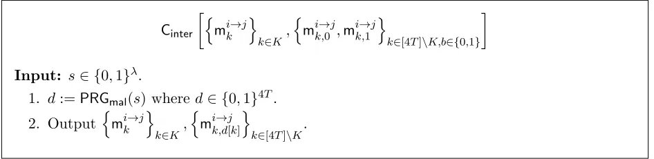
3. A pseudorandom generator PRG:{0,1}λ → {0,1}4T.
Parties: P1, P2, . . . , Pn. Inputs:
• P1 (also called as the receiver) inputs s∈ {0,1}λ and rlab2, . . . ,rlabn where each rlabi is
a collection of labels{rlabij,→01,rlabij,→11}j∈[λ2] with each label of lengthλ.
• For each i∈ [2, n], Pi (also called as the sender) inputs slabi, where slabi is a collection
of labels {slabij,→01,slabij,→11}j∈[λ]with each label having length λ.
Output: {Projection(Projection(s,slabi),rlabi)}i∈[2,n].
Figure 3: The function g computed by the internal MPC whereP1 acts as the receiver
Notations. For a bit string c, we use c[i] to denote the i-th bit of it. For each t ∈ [T] and
α, β ∈ {0,1}, we use (t, α, β) to succinctly denote the integer 4t+ 2α+β−3. In particular, we use c[(t, α, β)] to denote c[4t+ 2α+β −3] for any c ∈ {0,1}4T. We use lab to denote the set of
both labels per input wire of a garbled circuit, andlabf denotes the set of one label per input wire. Recall the definition of Projectionfrom Section 3.
We give an overview of the construction below and describe the formal construction later.
Overview. As explained in Section 2, our construction combines a special purpose OT extension protocol (which is delegatable, fine-grained secure and satisfies key availability) along with the two-round MPC protocols of [BL18, GS18] to obtain a protocol that minimizes the number of public key operations. Recall that the protocols of [BL18, GS18] used the concept of “talking garbled circuits” to squish the round complexity of a conforming protocol to two rounds. At a high level, in the first round, every pair of parties sets up a channel to enable their garbled circuits to interact, and then in the second round, they send “talking garbled circuits” that emulate the interactions in the conforming protocol. The interaction between the “talking garbled circuits” is done via oblivious transfer. In our new construction, we use a special purpose OT extension protocol that allows the parties to set-up the channel for interaction while minimizing the number of public key operations. A major modification from the description given in Section 2 is in modeling the special oblivious transfer as a protocol between a single receiver and n−1 senders. We do this to ensure that the receiver uses the same choice bits in interactions with every sender. Even though this is not an issue in the semi-honest case, it causes issues in the malicious setting if the corrupted receiver uses different choice bits in two different interactions. For uniformity of treatment, we adopt an approach where the special oblivious transfer is a protocol between a single receiver and n−1 senders.
Description of the Protocol. We give a formal description of our protocol below in the Fg
-hybrid model.
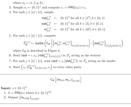
Round-1: Each partyPi does the following:
1. Compute (zi, vi)←pre(1λ, i, xi).
2. For eacht∈[T] and for each α, β ∈ {0,1}
whereφt= (?, f, g, h).
3. Samplesi← {0,1}λ and computeei:=PRG(si)⊕ci.
4. For eachj∈[n]\ {i}, sample
rlabjk,b→i ← {0,1}λ for all k∈[λ2], b∈ {0,1}
slabik,b→j ← {0,1}λ for all k∈[λ], b∈ {0,1}
mik,b→j ← {0,1}λ for all k∈[4T], b∈ {0,1}
5. For eachj∈[n]\ {i}, compute
e
CiB→j ←Garble
CB
n
mik,→0j,mik,→1j o
k∈[4T],b∈{0,1}
,
n slabik,b→j
o
k∈[λ],b∈{0,1}
whereCB is described in Figure 4.
6. Send (ssid=i, si,{rlabjk,b→i}j∈[n]\{i}) to Fg acting as the receiver.
7. For eachj∈[n]\ {i}, send (ssid=j,{slabik,b→j}) to Fg acting as the sender.
8. Send zi,{Ce
i→j
B }j∈[n]\{i}, ei
to every other party.
CB
h
{mk,0,mk,1}k∈[4T] i
Input: s∈ {0,1}λ.
1. d:=PRG(s) whered∈ {0,1}4T.
2. Outputmk,d[k] k∈[4T].
Figure 4: CircuitCB
Round-2: Each partyPi does the following:
1. Setsti := (z1k. . .kzn)⊕vi.
2. SetN =`+ 4T λ(n−1).
3. Setlabi,T+1 :={labk,i,T0+1,labi,Tk,1+1}k∈[N] wherelabi,Tk,b+1 := 0λ for each k∈[N], b∈ {0,1}. 4. foreach tfrom T down to 1 do:
(a) Parse φt as (i∗, f, g, h).
(b) Ifi=i∗ then compute (whereP is described in Figure 6)
e
Pi,t,labi,t
←Garble(1λ,P[i, φt, vi,⊥,lab i,t+1
]).
(c) If i 6= i∗ then for every α, β ∈ {0,1}, set m0α,β,0 = mi(→t,α,βi∗),e
i∗[(t,α,β)] and m
0
α,β,1 =
mi(→t,α,βi∗),1⊕e
i∗[(t,α,β)].
Computectiα,β := (m0α,β,0⊕labh,i,t0+1,m0α,β,1⊕labi,th,1+1) and compute
e
Pi,t,labi,t←Garble(1λ,P[i, φt, vi,{ctiα,β},lab i,t+1
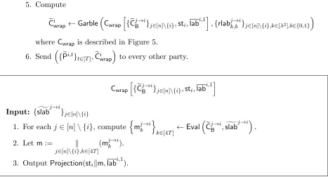
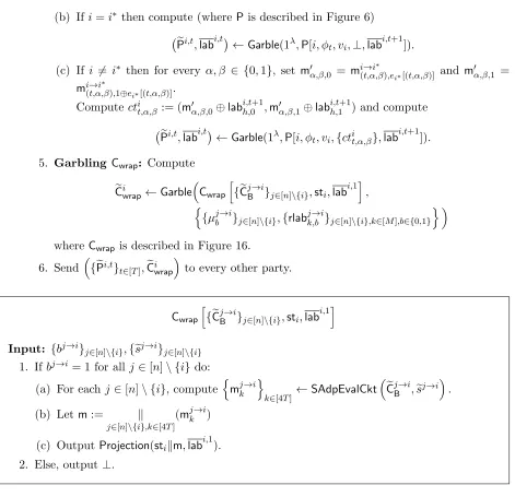
5. Compute
e
Ciwrap←GarbleCwrap
h
{Cej →i
B }j∈[n]\{i},sti,lab i,1i
,{rlabjk,b→i}j∈[n]\{i},k∈[λ2],b∈{0,1}
whereCwrap is described in Figure 5.
6. Send {Pei,t}t∈[T],Ceiwrap
to every other party.
Cwrap
h
{eC
j→i
B }j∈[n]\{i},sti,lab i,1i
Input: {slabg
j→i
}j∈[n]\{i}
1. For eachj∈[n]\ {i}, compute nmjk→io
k∈[4T]
←EvaleCj →i B ,slabg
j→i
.
2. Letm:= k
j∈[n]\{i},k∈[4T]
(mjk→i).
3. OutputProjection(stikm,lab i,1
).
Figure 5: Circuit Cwrap
Evaluation: Every party Pi does the following:
1. For eachj∈[n],
(a) Obtain (ssid=j,rlabg
j
) from Fg where partyPj acts as the receiver.
(b) labf
j,1
←Eval(Cejwrap,rlabg
j
)
2. foreach tfrom 1 to T do:
(a) Parse φt as (i∗, f, g, h).
(b) Compute ((α, β, γ),{ωj}j∈[n]\{i∗},labf
i∗,t+1
) :=Eval(Pei
∗,t ,labf
i∗,t
). (c) Set sti[h] :=γ⊕vi[h].
(d) foreach j6=i∗ do:
i. Compute (ct= (δ0, δ1),{labj,tk +1}k∈[N]\{h}) :=Eval(Pej,t,labf
j,t
).
ii. Recoverlabj,th +1 :=δγ⊕ωj.
iii. Set labf
j,t+1
:={labj,tk +1}k∈[N]. 3. Compute the output as post(i,sti).
Correctness. In order to prove correctness, it is sufficient to show that the labellabj,th +1computed in Step 2(d)ii of the evaluation procedure corresponds to the bit NAND(sti∗[f],sti∗[g])⊕vi∗[h].
Notice that by the structure of vi∗ we have for every j6=i∗,stj[f] =sti∗[f]⊕vi∗[f].
First, ωj is computed in Step 2b. Letk:= (t, α, β), and we haveωj =mkj→i∗ =mjk,PRG→i∗ (s
P
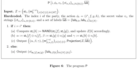
i, φt, vi,{ctα,β}α,β∈{0,1},lab
Input. Z =
sti,{mjk→i}j∈[n]\{i},k∈[4T]
.
Hardcoded. The index i of the party, the action φt = (i∗, f, g, h), the secret value vi, the
strings{ctα,β}α,β∈{0,1}, and a set of labels lab={labk,0,labk,1}k∈[N].
1. if i=i∗ then:
(a) Computesti[h] :=NAND(sti[f],sti[g]), and updateZ[h] accordingly.
(b) α:=sti[f]⊕vi[f], β:=sti[g]⊕vi[g] and γ:=sti[h]⊕vi[h].
(c) Output (α, β, γ),{mj(t,α,β→i )}j∈[n]\{i},Projection(Z,lab).
2. else:
(a) Output (ctsti[f],sti[g],{labk,Z[k]}k∈[N]\{h}).
Figure 6: The programP
Second, ct = (δ0, δ1) is computed in Step 2(d)i. Note that α = sti∗[f]⊕vi∗[f] = stj[f], β =sti∗[g]⊕vi∗[g] =stj[g]. From the functionality ofPj,t we know that ct=ctst
j[f],stj[g]=ct j α,β =
(m0α,β,0⊕labj,th,0+1,mα,β,0 1⊕labj,th,1+1) = (mjk,e→i∗
i∗[k]⊕lab j,t+1
h,0 ,m
j→i∗
k,ei∗[k]⊕1⊕lab j,t+1
h,1 ).
Therefore,δγ⊕ωj =mj→i
∗
k,ei∗[k]⊕γ⊕lab j,t+1
h,γ ⊕m j→i∗
k,PRG(si∗)[k]. Recall thatci
∗[k] =NAND(sti∗[f],sti∗[g])⊕ vi∗[h] =γ, thus ei∗[k]⊕γ =ei∗[k]⊕ci∗[k] =PRG(si∗)[k]. Henceδγ⊕ωj =labj,t+1
h,γ . This concludes
the proof.
It is useful to keep in mind that for every i, j ∈ [n] and k ∈ [`], we have that sti[k]⊕vi[k] =
stj[k]⊕vj[k]. Let us denote this shared value byst∗. Also, we denote the transcript of the interaction
in the computation phase byZ.
Efficiency. Let the number of public key operations in Φ benpkΦ and in one execution of Fg be
npkg. We choose the conforming protocol that performs OT extension between every pair of parties so that npkΦ is bounded by O(n2λ). The total number of public key operations in our two-round construction is O(npkΦ+n·npkg). It follows from Theorems 3.3 that this number is bounded by
poly(n, λ).
4.3 Simulator
Let A be a semi-honest adversary corrupting a subset of parties and let H ⊆ [n] be the set of honest/uncorrupted parties. Since we assume that the adversary is static, this set is fixed before the execution of the protocol. Below we provide the simulator.
SimΦ for Φ and the simulator Simckt for garbling scheme for circuits. Recall that A is static and
hence the set of honest parties H is known before the execution of the protocol.
Simulating the interaction withZ. For every input value for the set of corrupted parties that
S receives from Z,S writes that value to A’s input tape. Similarly, the output of A is written as the output on S’s output tape.
Simulating the interaction withA: For every concurrent interaction with the session identifier
sidthat Amay start, the simulator does the following:
• Initialization: S uses the inputs of the corrupted parties {xi}i6∈H and output y of the
functionality f to generate a simulated view of the adversary.5 More formally, for each
i ∈ [n]\H, S sends (input,sid,{P1· · ·Pn}, Pi, xi) to the ideal functionality implementing f
and obtains the outputy. Next, it executes SimΦ(1λ,{xi}i6∈H, y) to obtain{zi}i∈H (which is
the output of the pre-computation phase), the random tapes for the corrupted parties, the transcript of the computation phase denoted by Z∈ {0,1}t where Z[t] is the bit sent in the t-th round of the computation phase of Φ, and the value st∗ (where st∗[k] = sti[k]⊕vi[k] at
the end of the t-th round for each i∈[n] and k∈ [`]). S starts the real-world adversary A
with the random tape generated bySimΦ along with additional randomness used in execution of the two-round protocol.
• Round-1 messages from S to A: Next S generates CeB and eon behalf of honest parties as follows. For eachi∈H:
1. Sampleei← {0,1}4T.
2. For each j ∈ [n]\ {i}, sample mik→j ← {0,1}λ for all k∈ [4T]. Sample the slabi→j
k ←
{0,1}λ for eachk∈[λ] and compute
e
CiB→j ←Simckt
1λ,
n mik→j
o
k∈[4T],{slab
i→j k }k∈[λ]
.
3. Send zi,{Cei →j
B }j∈[n]\{i}, ei
to the adversary Aon behalf of the honest party Pi.
• Round-1 messages from A to S: Corresponding to everyi∈[n]\H,Sreceives from the adversaryAthe values
zi,{Cei →j
B }j∈[n]\{i}, ei
on behalf of the corrupted partyPi. Srecovers
the valuemik,b→j for all j∈[n]\ {i}, k∈[4T], b∈ {0,1}from random tape of party Pi.
• Messages from A to Fg: For every i∈ [n]\H, S receives (ssid = i, si,{rlab j→i
}j∈[n]\{i}) and
n
(ssid=j,slabi→j) o
j∈[n]\{i} that sends toFg.
• Round-2 messages from S to A: For each i∈ H, the simulator S generates the second round message on behalf of partyPi as follows:
1. Setlabf
i,T+1
:={labi,Tk +1}k∈[N]where labi,Tk +1:= 0λ for each k∈[N].
5For simplicity of exposition, we only consider the case where every party gets the same output. The proof in the
2. foreach tfrom T down to 1 do:
(a) Parse φt as (i∗, f, g, h).
(b) Setα∗ :=st∗[f], β∗ :=st∗[g], andγ∗ :=st∗[h]. (c) If i =i∗, then setmj(t,α→i∗,β∗) := m
j→i
(t,α∗,β∗),γ∗⊕e
i[(t,α∗,β∗)] for each j ∈[n]\H, sample
labi,tk ← {0,1}λ for each k∈[N] and compute
e
Pi,t ←Simckt
1λ,
(α∗, β∗, γ∗),{mj(t,α→i∗,β∗)}j∈[n]\{i},{labi,tk +1}k∈[N]
,{labi,tk }k∈[N]
.
(d) If i 6= i∗, then set δγ∗ := labi,t+1
h ⊕mi
→i∗
(t,α∗,β∗), sample δ1−γ∗ ← {0,1}λ, set ct :=
(δ0, δ1), samplelabi,tk ← {0,1}λ for each k∈[N] and compute
e
Pi,t ←Simckt
1λ,ct,{labki,t+1}k∈[N]\{h}
,{labi,tk }k∈[N]
.
3. Samplerlabik← {0,1}λ for each k∈[(n−1)λ2] (note that (n−1)λ2 is the length of the input to Cwrap) and compute
e
Ciwrap←Simckt
1λ,{labi,k1}k∈[N],{rlabik}k∈[(n−1)λ2]
.
4. Send
{Pei,t}t∈[T],Ceiwrap
to every other party.
• Messages fromFgtoA: For everyi∈H,Ssends (ssid=i,{rlabik}k∈[(n−1)λ2]) toAon behalf
ofFg. For everyi∈[n]\H, letslabg
j→i
:=Projection(si,slab j→i
) for each j∈[n]\H; for each
j∈H, defineslabg
j→i
:={slabjk→i}k∈[λ];Ssends (ssid=i,{Projection(slabg
j→i
,rlabj→i)}j∈[n]\{i})
toAon behalf of Fg.
• Round-2 messages fromAtoS: For everyi∈[n]\H,Sobtains the second round message from Aon behalf of the corrupted parties. Subsequent to obtaining these messages, for each
i∈H,Ssends (generateOutput,sid,{P1· · ·Pn}, Pi) to the ideal functionality.
4.4 Proof of Indistinguishability
We now show that no environment Z can distinguish whether it is interacting with a real world adversaryA or an ideal world adversaryS. We prove this via an hybrid argument.
• H0: This hybrid is the same as the real world execution.
• H1: In this hybrid, the functionalityFgis emulated by the simulatorSfaithfully. This hybrid is identical toH0.
• H2: In this hybrid, we change how theFg functionality is emulated by the simulator in every
call where i ∈ H is acting as the receiver. In particular, for any ssid = i ∈ H, party Pi
does not send
si,{rlabjk,b→i}j∈[n]\{i}
to the ideal functionality. Instead, the simulator uses
si,{rlabjk,b→i}j∈[n]\{i}
• H3: In this hybrid, we change how the Fg functionality is emulated by the simulator in every call where i ∈ H is acting as the sender. In particular, for any ssid = j ∈ [n], when
i∈H is acting as the sender in this execution, partyPi does not send{slabik,b→j}to the ideal
functionality. Instead, the simulator uses {slabik,b→j} to directly compute the output. This hybrid is distributed identically toH2.
• H4: In this hybrid we change Cei →j
B sent from S toA on behalf of the honest parties i∈ H
and the messages fromFg toA as follows.
We start by executing the protocol Φ on the inputs and the random coins of the honest and the corrupted parties. This yields a transcript Z∈ {0,1}T of the computation phase. Since
the adversary is assumed to be semi-honest the execution of the protocol Φ with A will be consistent withZ. In hybridH4 we make the following changes with respect to hybrid H3:
– In Round 1, for each i ∈ H, S generates {eC
i→j
B } on behalf of party Pi as follows: For
each j ∈[n]\ {i}, t∈[T], α, β ∈ {0,1}, letk= (t, α, β), setmki→j :=mik,PRG→j (s
j)[k] where {mik,→0j,mik,→1j} are the honestly generated masking strings. Sample the garbled circuit
labelsslabg
i→j
randomly and compute
e
CiB→j ←Simckt
1λ,nmik→jo
k∈[4T], g slabi→j
.
– Messages fromFgtoA: For eachi∈[n], j∈[n]\H: letslabg
j→i
:=Projection(si,slab j→i
).
For each i∈[n], Ssends (ssid=i,{Projection(slabg
j→i
,rlabj→i)}j∈[n]\{i}) to Aon behalf
of Fg.
The indistinguishability between H3 and H4 follows from|H| invocations of the security of garbled circuits. In particular, for any s,mk,0,mk,1 ∈ {0,1}λ for k ∈ [4T], the following distributions are computationally indistinguishable:
n Garble
1λ,CB
h
{mk,0,mk,1}k∈[4T],slab i
,Projection(s,slab) o
c
≈nSimckt
1λ,CB(s),slabg
,slabg o
=nSimckt
1λ,{mk}k∈[4T],slabg
,slabg o
where slabare randomly generated input keys for the garbled circuit (including both labels per input wire), andslabg are randomly generated labels for the garbled circuit (consisting of one label per input wire).
• H5: In this hybrid we change Ceiwrap sent from S to A on behalf of the honest parties i∈H and the messages fromFg toA as follows.
– In Round 2, for eachi∈H,Sgenerates Ceiwrap on behalf of partyPi as follows:
1. For eachi∈[n]\H, j∈[n]\ {i}, computemjk→i :=CjB→i(si).
2. Setm:= k
j∈[n]\{i},k∈[4T]
3. Sample the garbled circuit labelsrlabg
i
randomly and compute
e
Ciwrap←Simckt
1λ,Projection(stikm,lab i,1
),rlabg
i
wherelabi,1 are the honestly generated input labels of Pei,1.
– Messages from Fg to A: For everyi∈H, S sends (ssid =i,rlabg
i
) to A on behalf of
Fg. For every i∈ [n]\H, let slabg
j→i
:= Projection(si,slab j→i
) for each j ∈ [n]\H; S
sends (ssid=i,{Projection(slabg
j→i
,rlabj→i)}j∈[n]\{i}) to A on behalf ofFg.
The indistinguishability between H4 and H5 follows from|H| invocations of the security of garbled circuits. In particular, for any{eCj
→i
B }j∈[n]\{i},sti,lab i,1
,{slabg
j→i
}j∈[n]\{i}, we have
n Garble
1λ,Cwrap
h
{eCj →i
B }j∈[n]\{i},sti,lab i,1i
,{rlabj→i}j∈[n]\{i}
,
{Projection(slabg
j→i
,rlabj→i)}j∈[n]\{i}o
c
≈nSimckt
1λ,Cwrap({slabg
j→i
}j∈[n]\{i}),rlabg
i
,rlabg
io
= n
Simckt
1λ,Projection(stikm,lab i,1
),rlabg
i
,rlabg
io
where{rlabj→i}j∈[n]\{i} are randomly generated input keys for the garbled circuit (including both labels per input wire), and rlabg
i
are randomly generated labels for the garbled circuit (consisting of one label per input wire).
• H05+t(wheret∈ {1, . . . T}): The hybridsH05+tandH5+t(which we will describe later) are the
same asH4+texcept that we change the garbled circuits (from the second round) that play a role in the execution of thet-th round of the protocol Φ; namely, the actionφt= (i∗, f, g, h).
Let st∗ be the local state at the end of the t-th round of execution, and set α∗ := st∗[f],
β∗ := st∗[g], and γ∗ := st∗[h]. Hybrid H05+t is the same as hybrid H4+t except the changes below.
– If i∗ ∈/ H then skip the changes. In the second round, S generates Pei
∗,t
on behalf of
Pi∗: Set mj→i ∗
(t,α∗,β∗):=m
j→i∗
(t,α∗,β∗),γ∗⊕e
i∗[(t,α∗,β∗)] for eachj ∈[n]\H. Compute mas in H4,
sample the garbled circuit input labels labf
i∗,t
randomly, and compute
e
Pi∗,t ←Simckt
1λ,
(α∗, β∗, γ∗),{mj(→t,αi∗∗,β∗)}j∈[n]\{i∗},Projection(sti∗km,labi ∗,t+1
)
,labf
i∗,t
wherelabi
∗,t+1
are the honestly generated input labels ofPei
∗,t+1
.
The indistinguishability betweenH0
5+tand H4+tfollows directly from the security of garbled
circuits.
• H5+t (wheret∈ {1, . . . T}): HybridH5+tis the same as H0
– For each i ∈ H and i 6= i∗, S generates Pei,t on behalf of Pi: Set δγ∗ := labi,t+1
h ⊕
mi→i∗
(t,α∗,β∗),γ∗⊕e
i∗[(t,α∗,β∗)], sampleδ1−γ
∗← {0,1}λ, setct:= (δ0, δ1). Computemas in H4
and labf
i,t+1
:=Projection(stikm,lab i,t+1
) where labi,t+1 are the honestly generated input
labels of ePi,t+1. Sample the garbled circuit input labels labf
i,t
randomly and compute
e
Pi,t ←Simckt
1λ,
ct,{labi,tk+1}k∈[N]\{h}
,labf
i,t
.
Notice that here we sample δ1−γ∗ ← {0,1}λ instead of labi,t+1
h ⊕mi
→i∗
(t,α∗,β∗),1⊕γ∗⊕e
i∗[(t,α∗,β∗)].
Sincemi(→t,αi∗∗,β∗),1⊕γ∗⊕e
i∗[(t,α∗,β∗)] never appears anywhere else, lab i,t+1
h is information
theoreti-cally hidden, hence changingδ1−γ∗ to be randomly sampled does not change the distribution.
The rest of the indistinguishability proof betweenH5+tandH05+tfollows from the security of
garbled circuits.
• H6+T: Hybrid H6+T is the same as H5+T except that in the first round, S samples ei ←
{0,1}4T for eachi∈H instead ofPRG(s i)⊕ci.
Notice that in hybridH5+T, for eachi∈H,si and ci is only used to generate ei. Hence the
indistinguishability between H6+T and H5+T follows from |H| invocations of the security of the pseudorandom generatorPRG.
• H7+T: In this hybrid we just change how the transcriptZ,{zi}i∈H, random coins of corrupted
parties and valuest∗ are generated. Instead of generating these using honest party inputs we generate these values by executing the simulatorSimΦ on input{xi}i∈[n]\H and the outputy
obtained from the ideal functionality.
The indistinguishability between hybrids H7+T and H6+T follows directly from the
semi-honest security of the protocol Φ. Finally note thatH6+T is same as the ideal execution (i.e.,
the simulator described in the previous subsection).
5
Special Zero-Knowledge Protocol
In this section, we define and construct a special zero-knowledge protocol which will later be used in our construction against malicious adversaries. We give the formal definition below.
Definition 5.1 A special zero-knowledge protocol is a two-round protocol that securely realizes the FZK functionality given in Figure 7. Further, we require the number of pubic key operations performed in the protocol to be bounded by poly(n, λ) independent of the size of x and w.
We give a proof of the following theorem.
Theorem 5.2 Assuming the existence of two-round UC secure oblivious transfer, there exists a construction of special zero-knowledge protocol.
5.1 Construction
FZK parameterized by anNP relationR, running withn partiesP1, P2, . . . , Pn (of which some
may be corrupted) and an adversary S, proceeds as follows:
• P1 sends (prover,sid, x, w) to the functionality. The functionality sends (request, x, R(x, w)) to S. If S has corrupted P2, then S sends (response, µ) to the ideal functionality, and the ideal functionality broadcasts (R(x, w), x, µ) to every other party and goes offline. Else, P2 sends (verifier,sid, µ0, µ1) to the functionality, where
µb ∈ {0,1}λ.
• Upon receiving the inputs from both P1 and P2, functionality checks if R(x, w) = 1. If yes, it sends (1, x, µ1) to every party. Otherwise, it sends (0, x, µ0) to all parties.
Figure 7: Special Zero-Knowledge FunctionalityFZK
1. Special Non-interactive Statistically Binding Commitment. We use a special non-interactive, statistically binding commitment scheme (com,decom) where the length of the randomness used to commit to arbitrary length messages is λ. We note that any standard commitment can be made to satisfy this property by using a pseudorandom generator to expand the random string to required length.
2. Blum’s Hamiltonicity Protocol. We use the three-round, constant soundness zero-knowledge (zk1,zk2,zk3) protocol of Blum. We note that in Blum’s protocolzk2 ∈ {0,1}and we letzk3,b
be the response when zk2 = b. We also assume without loss of generality that zk1 includes the instance.
3. Two-Round Secure Computation Protocol. We make use of the two-round secure computation protocol of [GS18] (that can be based on any two-round UC secure oblivious transfer) computing the ideal functionalityFf described in Figure 10.
4. Length Doubling Pseudorandom Generator: We use a pseudorandom generatorPRG:
{0,1}λ → {0,1}2λ.
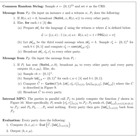
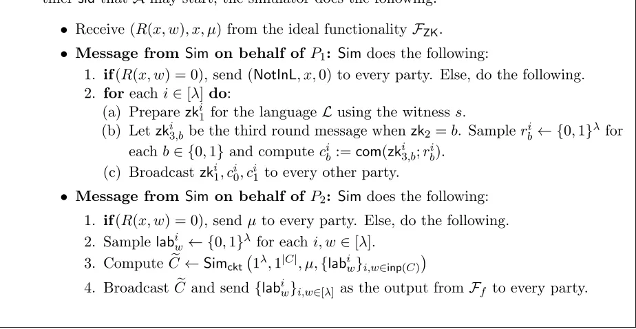
Overview. We give an overview of our construction of the two-round special zero-knowledge protocol below, and present the formal construction in theFf hybrid model in Figure 8.
In the first round, the prover computes Blum’s proof zk1,zk3,0,zk3,1 for the proofw, and com-putes the commitment (c0, c1) of (zk3,0,zk3,1) using randomness (r0, r1) respectively. It then sends (zk1, c0, c1) to the verifier. In the second round, the verifier samples a random bit b← {0,1}, and constructs a circuitC that has (b,zk1, c0, c1, µ0, µ1) hardwired in it. The circuitC takesr as input, checks ifr decommitscb and if (zk1, b,zkb) is a valid proof. If both checks pass, then it outputsµ1;
otherwise it outputsµ0. The verifier garbles the circuit C and sends Ce to the prover.
Additionally, the prover and verifier in parallel run a two-round MPC protocol to compute the labels for evaluating the garbled circuit Ce. Specifically, they jointly compute a function f which takes as input (r0, r1) from the prover andbalong with the input labels forCe from the verifier, and outputs the labels that correspond to rb. Thus, at the end of the protocol, all parties can obtain
Common Random String: Sampleσ ← {0,1}2λ and setσ as the CRS.
Message from P1: On input an instancex and a witness w,P1 does the following:
1. IfR(x, w) = 0, broadcast (NotInL, x, R(x, w)) to every other party. 2. Else,for each i∈[λ]do:
(a) Prepare zki1 for the language L using the witnessw whereL is defined below.
L:={(x, σ) :∃ (w, s) s.t. R(x, w) = 1∨PRG(s) =σ}
(b) Let zki3,b be the third round message when zki2 = b. Sample rib ← {0,1}λ for
eachb∈ {0,1} and computecib :=com(zki3,b;rbi). (c) Broadcast zki1, ci0, ci1 to every other party.
Message from P2: On input the message fromP1 :
1. If P1 has sent (NotInL, x,0), broadcast µ0 to every other party and every party outputs (0, x, µ0). Else, do:
(a) Sample ch← {0,1}λ.
(b) Samplelabiw,b ← {0,1}λ for each i, w∈[λ] and b∈ {0,1}.
(c) Compute Ce ← Garble(C[ch,{zki1, ci0, ci1}i∈[λ],{µb}b∈{0,1}],{labiw,b}) where the C is described in Figure 9.
(d) BroadcastCe to every party.
Internal MPC: The parties in parallel call Ff to jointly compute the function f shown in Figure 10. More specifically,P1sends{r0i, r1i}i∈[λ]toFf;P2sendsch,{labiw,b}i,w∈[λ],b∈{0,1}
to Ff; and P3, P4, . . . , Pn send nothing. Every party then gets {labiw}i,w∈[λ] back from
Ff.
Evaluation: Every party does the following: 1. Compute (b, x, µ)←EvalC,e {labiw}i,w∈[λ]
2. Output (b, x, µ).
Figure 8: Special Zero-Knowledge Protocol ΠZK
C
ch,{zki1, ci0, ci1}i∈[λ],{µb}b∈{0,1}
Input: r1, r2, . . . , rλ.
Hardcoded parameters: ch,{zki1, ci0, ci1}i∈[λ],{µb}b∈{0,1}
1. Use the randomness ri to obtain the messagezki
3 committed in cich[i]for each i∈[λ]. 2. For each i∈[λ], check if (zki1, ch[i],zki3) is a valid proof for the membership in language
L.
3. If any of the checks fails, output (0, x, µ0). Else, output (1, x, µ1).
Figure 9: Circuit C
Parties: P1, P2, . . . , Pn. Inputs:
• P1 inputs{ri0, r1i}i∈[λ], whererib ∈ {0,1}λ.
• P2 inputsch,{labiw,b}i,w∈[λ],b∈{0,1}, wherelabiw,b∈ {0,1}λ.
• P3, P4, . . . , Pn input nothing. Output: {labiw,ri
ch[i][w]
}i,w∈[λ] (same for every party).
Figure 10: The Function f Computed by the Internal MPC
Correctness. To argue the correctness of the protocol, we only need to prove that in the eval-uation step, µ is either µ0 or µ1 based on whether R(x, w) = 0 or R(x, w) = 1. We know that the output ofFf is
labiw i,w∈[λ], wherelabiw=labiw,ri ch[i][w]
. Notice thatlabiw,b’s are the input keys
of Ce, hence labiw is the label corresponding to the w-th bit of rchi [i]. Using these input labels to
evaluateCe gives us Eval
e
C,
labiw i,w∈[λ]=C
n
rchi [i]o i∈[λ]
.
In the circuit evaluation ofC,rich[i]is used to obtainzk3i,ch[i]fromcich[i]. It now follows from the completeness of (zki1, ch[i],zki3,ch[i]) that µis either µ0 orµ1 based onR(x, w) = 0 orR(x, w) = 1.
Efficiency. The number of public key operations performed in the protocol is poly(n, λ) which follows from Theorem 3.3 when applied to functionf.
5.2 Security