AN INTEGRAL EQUATION METHOD FOR SOLVING NEUMANN
PROBLEMS ON SIMPLY AND MULTIPLY CONNECTED REGIONS WITH
SMOOTH BOUNDARIES
(KAEDAH PERSAMAAN KAMIRAN UNTUK PENYELESAIAN MASALAH
NEUMANN ATAS RANTAU TERKAIT RINGKAS DAN BERGANDA
DENGAN SEMPADAN LICIN)
ALI HASSAN MOHAMED MURID MUNIRA ISMAIL
MOHAMED M.S. NASSER HAMISAN RAHMAT UMMU TASNIM HUSIN
AZLINA JUMADI
EJAILY MILAD AHMAD ALEJAILY CHYE MEI SIAN
RESEARCHVOTE NO: 78316
Department of Mathematics Faculty of Science Universiti Teknologi Malaysia
&
Ibnu Sina Institute for Fundamental Science Studies Faculty of Science
Universiti Teknologi Malaysia
Acknowledgement
ABSTRACT
(Keywords: Laplace’s equation, Dirichlet problem, Neumann problem, multiply connected region, boundary integral equation, generalized Neumann kernel)
This research presents several new boundary integral equations for the solution of Laplace’s equation with the Neumann boundary condition on both bounded and unbounded multiply connected regions. The integral equations are uniquely solvable Fredholm integral equations of the second kind with the generalized Neumann kernel. The complete discussion of the solvability of the integral equations is also presented. Numerical results obtained show the efficiency of the proposed method when the boundaries of the regions are sufficiently smooth.
Key Researchers:
Assoc. Prof. Dr. Ali Hassan Mohamed Murid Assoc. Prof. Dr. Munira Ismail
Assoc. Prof. Dr. Mohamed M.S. Nasser Tn. Hj. Hamisan Rahmat
Cik Ummu Tasnim Husin Pn. Azlina Jumadi
Mr. Ejaily Milad Ahmad Alejaily Cik Chye Mei Sian
E-mail :[email protected] Tel. No. : 07-5534245
ABSTRAK
(Katakunci: Persamaan Laplace, masalah Dirichlet, masalah Neumann, rantai terkait berganda, persamaan kamiran, inti Neumann teritlak)
Penyelidikan ini menghasilkan beberapa persamaan kamiran baru untuk penyelesaian persamaan Laplace dengan syarat sempadan Neumann atas rantau terkait berganda yang terbatas dan tak terbatas. Persamaan kamiran ini merupakan persamaan kamiran Fredholm jenis kedua dengan inti Neumann teritlak yang memiliki penyelesaian unik. Perbincangan mengenai kebolehselesaian persamaan kamiran ini turut disampaikan. Keputusan berangka yang diperoleh menunjukkan keberkesanan kaedah yang dipersembahkan jika sempadan rantau adalah licin secukupnya.
Penyelidik Utama:
Prof. Madya Dr. Ali Hassan Mohamed Murid Prof. Madya Dr. Munira Ismail
Prof. Madya Dr. Mohamed M.S. Nasser Tn. Hj. Hamisan Rahmat
Cik Ummu Tasnim Husin Pn. Azlina Jumadi
En. Ejaily Milad Ahmad Alejaily Cik Chye Mei Sian
E-mail :[email protected] Tel. No. : 07-5534245
CHAPTER TITLE
TITLE PAGE
ACKNOWLEDGEMENT ABSTRACT
ABSTRAK
TABLE OF CONTENTS LIST OF TABLES LIST OF FIGURES LIST OF APPENDICES
PAGE
i ii iii iv v ix xi xii
1 INTRODUCTION
1.1 General Introduction 1.2 Background of the Problem 1.3 Statement of the Problem 1.4 Objectives of the Research 1.5 Importance of the Research 1.6 Scope of the Research 1.7 Outline of Report
1 1 3 3 4 4 5 5
2 AN INTEGRAL EQUATION METHOD FOR
SOLVING NEUMANN PROBLEMS ON SIMPLY CONNECTED SMOOTH REGIONS 2.1 Introduction
2.2 Auxiliary Material
2.2.1 The Neumann Problem
2.2.2 The Riemann-Hilbert Problem
2.2.3 Integral Equation for Interior
Riemann-7
Hilbert Problem
2.3 Reduction of the Neumann Problem to the Riemann-Hilbert Problem
2.3.1 Integral Equation for Solving Interior Neumann Problem
2.4 Numerical Implementation 2.5 Examples
2.6 Conclusion
15
16
17 19 24
3 AN INTEGRAL EQUATION METHOD FOR
SOLVING EXTERIOR NEUMANN PROBLEMS ON SIMPLY CONNECTED REGIONS
3.1 Introduction 3.2 Auxiliary Material
3.2.1 Definition of Normal Derivative 3.2.2 The Exterior Riemann-Hilbert Problem 3.2.3 Integral Operators
3.2.4 Integral Equation for the Exterior Riemann-Hilbert Problem
3.3 Modification of the Exterior Neumann Problem
3.3.1 Reduction of the Exterior Neumann Problem to the RH Problem 3.3.2 Modified Integral Equation for the
Exterior RH Problem
3.4 Numerical Implementations of the Boundary Integral Equation
3.4.1 Examples
25
25 26 27 28 30 31
33
33
34
37
3.5 Conclusion 42
4 A BOUNDARY INTEGRAL EQUATION FOR
THE INTERIOR NEUMANN PROBLEM ON MULTIPLY CONNECTED SMOOTH
REGIONS 4.1 Introduction 4.2 Auxiliary Material 4.2.1 Neumann Kernels 4.2.2 The Neumann Problem
4.2.3 The Riemann-Hilbert Problem
4.2.4 Integral Equation for the RH Problem 4.3 A Boundary Integral Equation for the
Neumann Problem
4.3.1 Reduction of the Neumann Problem to the RH Problem
4.3.2 Solvability of the RH Problem and Derived Integral Equation
4.4 Numerical Implementation 4.5 Examples
4.6 Conclusion
43
43 44 45 46 47 49 50
50
51
52 53 56
5 A BOUNDARY INTEGRAL EQUATION FOR
THE EXTERIOR NEUMANN PROBLEM ON MULTIPLY CONNECTED SMOOTH
REGIONS 5.1 Introduction 5.2 Auxiliary Material
5.2.1 Boundary Integral Equation for Solving Exterior Neumann Problem
57
6
5.2.2 Boundary Integral Equation for Solving Exterior Riemann-Hilbert Problem 5.2.3 The Riemann-Hilbert Problem
5.2.4 The Solvability of the Riemann-Hilbert Problem
5.3 Modification of the Exterior Neumann Problem
5.3.1 Reduction of the Exterior Neumann Problem to the Exterior Riemann-Hilbert Problem
5.3.2 Integral Equation Related to the Exterior Riemann-Hilbert Problem
5.3.3 The Solvability of the Exterior Riemann-Hilbert Problem
5.3.4 Modified Integral Equation for the Exterior Riemann-Hilbert Problem 5.3.5 Modifying the Singular Integral Operator 5.3.6 Computing f(z) and f’(z)
5.4 Numerical Implementations of the Boundary Integral Equation
5.5 Examples 5.6 Conclusion
CONCLUSION AND SUGGESTIONS 6.1 Conclusion
6.1.1 Name of Articles/ Manuscript/ Books Published
6.1.2 Title of Paper Presentations (international/ local)
6.1.3 Human Capital Development
63
65 67
69
69
71
72
73
76 78 79
81 86
87 87 88
89
6.2 Suggestions for Future Research 90
LIST OF TABLES
TABLE NO.
2.1
2.2
3.1
3.2
3.3
3.4
4.1
4.2
5.1
5.2
TITLE
Numerical results for Examples 2.1 and 2.2
Numerical results for Examples 2.1 and 2.2
The error f'(z) f'n(z) for the exterior Neumann problem on the boundary 1,2,and3
The error f(z) fn(z)for the exterior Neumann problem on the boundary1.
The error f(z) fn(z) for the exterior Neumann problem on the boundary2.
The error f(z) fn(z) for the exterior Neumann problem on the boundary3.
The error u(z)un(z) for Example 4.1
The error u(z)un(z) for Example 4.2
The error f(z) fn(z) for Example 5.1
The error u(z)un(z) for Example 5.1
PAGE
24
24
42
42
42
43
56
57
84
5.3
5.4
5.5
5.6
The error f(z) fn(z) for Example 5.2
The error u(z)un(z) for Example 5.2
The error f(z) fn(z) for Example 5.3
The error u(z)un(z) for Example 5.3
86
86
87
LIST OF FIGURES
FIGURE NO.
2.1 2.2 2.3 3.1 3.2 3.3 3.4 4.1 4.2 4.3 5.1 5.2 5.3 5.4 5.5
TITLE
A Neumann problem in region An ellipse
An Oval of Cassini
The exterior Neumann problem
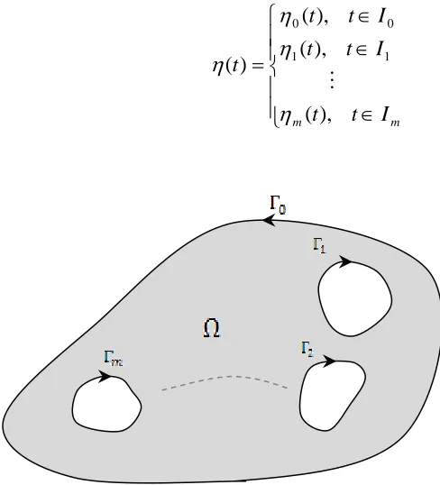
The curve 1and the exterior test points The curve 2and the exterior test points The curve 3and the exterior test points Bounded multiply connected region The test region 1 for Example 4.1 The test region 2 for Example 4.2 Unbounded multiply connected region
An unbounded multiply connected region G of connectivity The test region 1 for Example 5.1
The test region 2 for Example 5.2
The test region 3 for Example 5.3
PAGE
10 19 21 28
40
LIST OF APPENDICES
APPENDIX NO.
A
TITLE
Publications
PAGE
CHAPTER 1
RESEARCH FRAMEWORK
1.1 General Introduction
A popular source of integral equations has been the study of elliptic partial differential equations. It is also well known from books on the equations of mathematical physics that the basic boundary value problems for the Laplace equation are solved by means of the so-called potentials of simple and double layers (Gakhov, 1966). There are two of them; the Dirichlet problem and the Neumann problem. Given a boundary value problem for an elliptic partial differential equation over region D, the problem can often be reformulated as an equivalent integral equation over the boundary of D. Such a reformulation is called a boundary integral equation (Atkinson, 1997). As an example of such a reformulation, Carl Neumann investigated the solvability of some boundary integral equation reformulations for Laplace‟s equation, thereby also obtaining solvability results for Laplace‟s equation.
use of finite difference and finite element methods. Since 1970, there has been a significant increase in the popularity of using boundary integral equations to solve Laplace‟s equation and many other elliptic equations, including the biharmonic equation, the Helmholtz equation, the equations of linear elasticity and the equations for Stokes‟ fluid flow (Atkinson, 1997).
Solving the Neumann problem by the boundary integral equation method is one of the classical methods. The classical boundary integral equations for the Neumann problems are the two Fredholm integral equations of second kind with the Neumann kernel. The solutions of the Neumann problems are represented as the potential of a single layer as the way of deriving these boundary integral equations (Nasser, 2007). In general, the Neumann kernel usually appears in the integral equations related to the Dirichlet problem, the Neumann problem and conformal mappings (Ismail, 2007).
However, the integral equation for the interior Neumann problem is not uniquely solvable since the lack of unique solvability for the Neumann problem itself. The simplest way to deal with the lack of uniqueness in solving the integral equation is to introduce an additional condition (Atkinson, 1997) which lead to a unique solution. There are other ways of converting integral equation to a uniquely solvable equation. By using Kelvin transform, the interior Neumann problem can be converted to an equivalent exterior problem. This seems to be a very practical approach in solving interior Neumann problems, but it does not appear to have been used much in the past.
1.2 Background of the Problem
A Neumann problem is a boundary value problem for determining a harmonic function
x yu , interior or exterior to a region with prescribed values of its normal derivative u n on the boundary.
Applications of Neumann problems abound in classical mathematical physics. Some examples are heat problems in an insulated plate, electrostatic potential in a cylinder and potential of flow around airfoil. If the region is a disk, exact solution formula for the Neumann problem is known and the formula is called Dini‟s formula. For arbitrary simply connected region, the solution formula requires conformal mapping.
A more direct approach that avoid conformal mapping is the boundary integral equation method for solving the Neumann problem. Recently, Nasser (2007) has developed two integral equations with the generalized Neumann kernel that can provide the boundary values of the solution of the Neumann problem. Nasser‟s method is based on an earlier works by Murid and Nasser (2003) and Wegmann et al. (2005) related to the Riemann problem and Dirichlet problem.
1.3 Statement of the Problem
1.4 Objectives of the Research
The objectives of this research are to:
i. study the Neumann problem and the Riemann-Hilbert problem as well as integral equations for Riemann-Hilbert problem on multiply connected regions.
ii. reduce the interior and exterior Neumann problems to the equivalent Riemann-Hilbert problems.
iii. derive the boundary integral equations related to the interior and exterior Riemann-Hilbert problems.
iv. determine the solvability of the attained integral equations related to the Riemann-Hilbert problems.
v. perform numerical calculations for solving the boundary integral equations using softwares such as MATHEMATICA or MATLAB.
1.5 Importance of the Research
Knowledge on complex analysis in general and boundary integral equations in particular is still growing. There have been several studies on boundary integral equations with Neumann kernel related to Neumann problem. This research has developed non-singular integral equations with continuous kernel associated to Neumann problem on multiply connected regions with smooth boundaries. Furthermore, the analysis of solvability for these integral equations are determined as well.
1.6 Scope of the Research
This research is mainly on the theoretical reduction of the Neumann problem to Riemann-Hilbert problem. The Neumann problem is then solved numerically using the integral equation related to Riemann-Hilbert problem. We are mainly concerned on the interior and exterior Neumann problems on multiply connected regions with smooth boundaries.
1.7 Outline of Report
This project consists of seven chapters. The introductory Chapter 1 details some discussion on the background of the problem, problem statement, objectives of research, importance of the research, scope of the study and chapters organization.
Chapter 2 presents some auxiliary materials related to the Neumann problem, the Riemann-Hilbert problems as well as integral equation for Riemann-Hilbert problems. In this chapter, we reduce the interior Neumann problem into the interior Riemann-Hilbert problem and construct the boundary integral equation for solving it. We discuss the question on how to treat the integral equations numerically. Some numerical examples are presented to show the effectiveness of the method.
Chapter 3 focuses on the development of a numerical method for the exterior Neumann problem in a simply connected smooth region. Firstly, we reduce the exterior Neumann problem to the exterior Riemann-Hilbert problem. Then, the boundary integral equation for the Neumann problem is derived based on the exterior Riemann-Hilbert problem. Numerical implementations of the derived integral equation are also presented.
Neumann kernel related to the Riemann-Hilbert problem (briefly, RH problem). This integral equation is the Fredholm integral equation of the second kind. Solvability of the integral equation is also discussed.
Numerical experiments on some test regions are also reported.
Chapter 5 deals with the reduction of exterior Neumann problem on a multiply connected region to the exterior Riemann-Hilbert problem. Thus this chapter extends the results of Chapter 3. We show how to reduce the exterior Neumann problem on multiply connected region into the exterior Riemann-Hilbert problem and derive the boundary integral equation for solving it. Then, we provide a numerical technique for solving the boundary integral equation and present some numerical examples on several test regions.
CHAPTER 2
AN INTEGRAL EQUATION METHOD FOR SOLVING NEUMANN PROBLEMS ON SIMPLY CONNECTED SMOOTH REGIONS
2.1 Introduction
A Neumann problem is a boundary value problem of determining a harmonic function interior or exterior to a region with prescribed values of its normal derivative on the boundary. Applications of Neumann problems abound in classical mathematical physics. Some examples are heat problems in an insulated plate, electrostatic potential in a cylinder, potential flow around airfoil. If the region is a disk, exact solution formula for the Neumann problem is known and the formula is called Dini‟s formula. For arbitrary simply connected region, the solution formula requires conformal mapping. A more direct approach that avoid conformal mapping is the boundary integral equation method for solving Neumann problem.
representing the solutions of the Neumann problems as the potential of a single layer. However, the integral equation for the interior Neumann problem is not uniquely solvable since the lack of unique solvability for the Neumann problem itself. The simplest way to deal with the lack of uniqueness in solving the integral equation is to introduce additional conditions (Atkinson, 1997).
Recently, Nasser (2007) proposes a new method to solve the interior and the exterior Neumann problems in simply connected regions with smooth boundaries. The method is based on two uniquely solvable Fredholm integral equations of the second kind with the generalized Neumann kernel.
This chapter is organized as follows: Section 2.2 presents some auxiliary materials related to the Neumann problem, the Riemann-Hilbert problems as well as integral equation for Riemann-Hilbert problems. In Section 2.3, we reduce the interior Neumann problem into the interior Riemann-Hilbert problem and construct the boundary integral equation for solving it. We will discuss the question on how to treat the integral equations numerically in Section 2.4. Some numerical examples are presented in Section 2.5. In Section 2.6, a short conclusion is given.
2.2 Auxiliary Material
Let be a bounded simply connected Jordan region with 0 (see Figure 2.1). The boundary is assumed to have a positively oriented parameterization
t where
t is a 2 -periodic twice continuously differentiable function with
t d/dt 0. The parameter t need not be the arc length parameter. The exterior of is denoted by . For a fixed with1
Hölder norm. A Hölder continuous function hˆ on can be interpreted via h
t hˆ
t as a Hölder continuous function h of the parameter t and vice versa.Let A
t be a continuous differentiable 2 -periodic function with A 0. We define two real kernels N and M by
, 1Re
, (2.1)
t t t
A A t
M
, 1Im
. (2.2)
t t t
A A t
N
The kernel N
,t is called a generalized Neumann kernel formed with A and . When A1 , the kernel N is the Neumann kernel which arises frequently in the integral equations for potential theory and conformal mapping.Lemma 2.1 (Wegmann et al., 2005)
a) The kernel N
,t is continuous with
. (2.3)2 1 Im 1
,
t A
t A t t t
t
N
b) The kernel M
,t has the representation
, , (2.4)2 cot 2
1
,t t M1 t
M
with the continuous kernel M1 which takes on the diagonal the values
. (2.5)2 1 Re 1 ,
1
t A
t A t t t
t M
, , (2.6)2
0
dt t t
N
N
, . (2.7)2
0
1 t t dt
M
1 M
Let also M and K be the singular integral operators
, , (2.8)2
0
dt t t
M
M
. (2.9)2 cot 2
1 2
0
dt t t
K
The integrals in (2.8) and (2.9) are principal value integrals. The operator K is known as the Hilbert transform. The operators N , M, M1 and K are bounded in Hand map H into H . It follows from (2.4) that
) 10 . 2 ( .
K M
M 1
Lemma 2.2 (Wegmann et al., 2005)
a) Let N be the generalized Neumann kernel formed with A1 and . Then 1 is not an eigenvalue of N.
2.2.1 The Neumann Problem
Interior Neumann problem. Let n be the exterior normal to and let H be a given function such that
2
0
0
d
. (2.11)
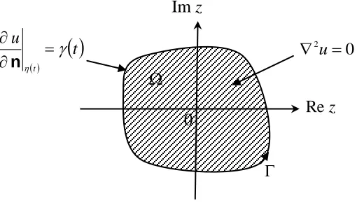
Find the function u harmonic in , Hölder continuous on and on the boundary , u satisfies the boundary condition (see Figure 2.1)
t t t u
,
n . (2.12) The interior Neumann problem is uniquely solvable up to an additive real constant (Atkinson,
1997). This arbitrary real constant is specified by assuming u
0 0.
t ut
n 0
2
u
Figure 2.1: A Neumann problem in region .
Lemma 2.3 (Atkinson, 1997)
The interior Neumann problem with the condition u
0 0 is uniquely solvable.
z Re z
Im
2.2.2 The Riemann-Hilbert Problem
Interior Riemann-Hilbert problem. Let CH and A be given functions. Find a function F analytic in , continuous on the closure , such that the boundary values Ffrom inside satisfy
t u t bt v t C
ta . (2.13)
Another frequently used form of writing the boundary condition is
,
, ( ) ( ) ( ).Re At F t Ct t At a t ib t
t
(2.14)
If C
t 0, then this equation is a non-homogeneous boundary condition, while if C
t 0, we have a homogeneous boundary condition, i.e.,
0,
.Re At F t t
t
(2.15)
Equation (2.13) is also equivalent to
2
,t A
t C t
F t A
t A t
F (2.16)
t at ibt .A (2.17)
So, we call equation (2.14) as the non-homogeneous interior Riemann-Hilbert problem and equation (2.15) as the homogeneous interior Riemann-Hilbert problem.
The solvability of the Riemann-Hilbert problem in a region depends upon the geometry of the simply connected region with smooth boundary as well as upon the index of
the function A(t) with respect to the boundary which is denoted by ind
A . (2.18)It is also regarded as the index of the Riemann-Hilbert problem (Gakhov, 1966).
Suppose that is a smooth Jordan curve and A
t is a continuous non-vanishing function given on . The index of the function A
t with respect to the curve is defined to be the increment of its argument in traversing the curve in the positive direction, divided by 2 . Then, the index of A
t can be written in the form
arg
. 21
ind
A At
(2.19)
The index can be expressed by the integral
ln
, 21 arg
2 1
ind
d At
i t
A d A
(2.20)
where the integral is understood in the sense of the Stieltjes (Gakhov, 1966). If the function A
t is continuously differentiable on , then
.2 1 ln
2 1
ind dt
t A
t A i t
A d i
A
(2.21)
2.2.3 Integral Equation for Interior Riemann-Hilbert Problem
Theorem 2.1 (Wegmann et al., 2005)
If F is the solution of the interior Riemann-Hilbert problem (2.14) with boundary values
A
t F
t C
t i
t , (2.22) then the imaginary part in (2.22) satisfies the integral equationNMC. (2.23)
Theorem 2.2 (Wegmann et al., 2005)
a) If 0 then the integral equation
N, (2.24)
has a solution if and only if R,where
: Re , , 0
.
G n
analytic i G
t G t A t
C H C
R
b) If 0 then the integral equation (2.24) has a unique solution for anyH.
2.3 Reduction of the Neumann Problem to the Riemann-Hilbert Problem
Suppose that u is a solution of the interior Neumann problem. Since u is harmonic function in , then u has a harmonic conjugate v in . Then f uiv is analytic in with derivative
f'ux ivx . (2.25)
The directional derivative of f in the direction of the outer unit normal vector to the path is given by (Husin, 2009)
t v i u t f n nn . (2.26)
Assuming
t x t iy t and applying nn
u u and
jy i x j t t x i t t
y
n n
n ' '
, we obtain
t y y iu y v i x x iv x u t f n nn . (2.27)
Applying (2.25) and Cauchy-Riemann equations, we get
t y i x f t f n nn ' . (2.28)
Taking the real parts of both sides and applying (2.12), the above equation becomes
t f t After substituting
tt i
n into (2.29), we get
Re
'
t t
f t i t
t
. (2.30)
Letting g i f' and
t t t we obtain
t tt g
t
Re , (2.31)
which is the interior Riemann-Hilbert problem. Comparison of (2.31) with (2.14) yields
t t ,A F
t g
t , and C(t)(t).2.3.1 Integral Equation for Solving Interior Neumann Problem
By Theorem 2.1, if g
t is the solution of the interior Riemann–Hilbert problem (2.31) with boundary values
t g
t
t i
t , (2.32)then the imaginary part in (2.32) satisfies the integral equation
NM , (2.33) i.e.
. 20 , 2
0
,
The solvability of the Riemann-Hilbert problem (2.31) is determined by the index of the function A
t which is defined as the winding number of A with respect to 0 . Applying (2.21) with A
t , we get
.1 2
1
d t
t i
(2.35)
By means of the Cauchy Integral Formula, we get 1.
Thus, by Theorem 2.2, integral equation (2.33) has a unique solution for M H and integral equation (2.33) is solvable for each CH.
2.4 Numerical Implementation
Since the functions A
t and
t are 2 -periodic, the integral operator N in (2.6) can be best discretized on an equidistant grid by the trapezoidal rule, i.e., the integral operator N is discretized by the Nyström method (Atkinson, 1997).Define the n equidistant collocation points ti by
1
2 , i 1,2,...,n. ni
ti (2.36)
Then, using the Nyström method with the trapezoidal rule to discretize the integral equation (2.33), we obtain the linear system
i ,n j
j n j i i
n N t t t t
n
t
M1
, 2
(2.37)
Defining the matrix Q[Qij] and vector x[xi] and y[yi] by
tii y i t n i x j t i t N n ij
Q 2 , , , M
,
equation (2.37) can be rewritten as an n by n system
I Q
x y. (2.38) For the calculation on the right-hand side of (2.37), we first calculate
ti ti ti , i1, 2,...,n. (2.39) Then, by using (2.10), we have
M
ti M1
ti K
ti (2.40) for i1, 2 ,...,n. The values of
K
ti will be calculated directly by usingMATHEMATICA package, i. e., CauchyPrincipalValue, while the values of
M1
ti will be calculated by using the trapezoidal rule, i. e.,
2
, ,1 1
1
n
j
j j i
i M t t t
n
t
M (2.41)
for i1, 2 ,...,n. Finally, (2.32) implies
ti f
ti
ti i n
tii
'
.
2.5 Examples
Example 2.1
For our examples, we use two boundary curves: an ellipse and the oval of Cassini. For ellipse, the boundary has the parametrization (see Figure 2.2).
t cost i5sint, 0 t 2π :1
,
Figure 2.2: An ellipse for Example 2.1
We choose a unique solution of the Neumann problem with condition u
0
0 as
z ex ye z xiyu cos , . (2.42)
For the above Neumann problem, the function
t is given by
t u t
n . (2.43)
i. e.,
t t
t t
e t t
t t
e
t t t
2 2
cos
2 2
cos
cos 25 sin
sin sin
5 sin cos
25 sin
cos 5 sin
5 cos
.
0 1 2 3 4 5
We now give a verification of (2.31).
t t t 5ecostcostcos
5sint
ecostsintsin
5sint
.
Now, we consider the left-hand side of equation (2.31) for the same region. We define the analytic function as
z f x y u x y iv
x yf , ( , ) , ,
where v(x,y)exsiny is a harmonic conjugate of u(x,y)excosye
f
t ecostcos
5sint
eiecostsin
5sint
. (2.44)Thus
f
t u iv e t
t
ie t
t
tx
x cos 5sin sin 5sin
' cos cos
. (2.45)
Multiplying this result with
t i , we have
t i f '
t
sinti5cost
ecostsin
5sint
iecostcos
5sint
.
which is equal to the right-hand side of (2.31). This completes the verification.
Example 2.2
For the oval of Cassini, the boundary parametrization is
t R
t eit, 0 t 2π :2
,
where R
t 2.52cos2t(see Figure 2.3).Figure 2.3: An oval of Cassini for Example 2.2
We again choose the unique solution of the Neumann problem with condition u
0
0 as u
z excosye, z xiy. (2.46)For this problem, the unit tangent vector
t t tT
, i. e.,
[ [
] sin ) ( ' cos ) ( cos
) ( ' sin ) (
] sin ) ( ' cos ) ( cos
) ( ' sin ) (
t t R t t R i t t R t t R
t t R t t R i t t R t t R t
t t
T
.
For the above Neumann problem, the function
t is given by,-1 0 1
-4 -3 -2 -1 0 1 2 3 4
'
5 cos cos
5sin
sin sin
5sin
,Re cos cos
t t
e t t
e t
f i
t
t t
' , ' ) ( t t x u t y u ut x y
n (2.47) i.e.,
. [ [ ] sin ) ( ' cos ) ( cos ) ( ' sin ) ( cos ) ( ' sin ) ( sin sin ] sin ) ( ' cos ) ( cos ) ( ' sin ) ( sin ) ( ' cos ) ( sin cos cos cos t t R t t R i t t R t t R t t R t t R t t R e t t R t t R i t t R t t R t t R t t R t t R e t t t R t t R We now give a verification of (2.31). The right-hand side of equation (2.31) for the second region is
.
e R t t R t t R t t
t t R t t R t t R e t t t t t R t t R cos ' sin sin sin sin ' cos sin cos cos cos
Now, we consider the left-hand side of equation (2.31) for the same region. Thus
f
t u iv eR t t
R
t t
ieR t t
R
t t
tx
x cos sin sin sin
' cos cos
. (2.48)
Multiplying the result with
t i , we have
cos sin sin sin
. sin ' cos cos ' sin ' cos cos t t R e t t R ie t t R t t R i t t R t t R t f i t t t R t t R
,
e Rt t Rt t R t t
t t R t t R t t R e
t f i t
t t R
t t R
cos ' sin sin
sin
sin ' cos sin
cos '
Re
cos cos
which is equal to the right-hand side (2.31). This completes the verification.
In Table 2.1 we calculate the sup-norm error
'
'
f
f n between the approximate boundary values of f
n
'
and the exact boundary values of f' at the node points for Examples 2.1 and 2.2. We also calculate the sup-norm error
x
n
x u
u between the approximate boundary values of uxn and the exact boundary values of ux at the node points. With the same reasoning, Table 2.2 presents the sup-norm errors
f
fn and
u
un for Examples 2.1 and 2.2.
Table 2.1: Numerical results for Examples 2.1 and 2.2
'
'
f f
n uxnux
n 1 2 1 2
32 1.14 (-05) 7.40 (-02) 3.56 (-06) 7.40 (-02) 64 9.17 (-11) 1.18 (-03) 7.49 (-12) 1.18 (-03)
128 - 5.73 (-07) - 5.73 (-07)
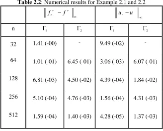
Table 2.2: Numerical results for Example 2.1 and 2.2
2.6 Conclusion
This chapter has presented a new integral equation for solving the interior Neumann problem in a simply connected region. The approach used in this paper to reduce the interior Neumann problem to an interior RH problem has been used before in (Henrici,p. 281, 1986). But the RH problem is solved in (Henrici, 1986) using a non-uniquely solvable integral equation (Henrici, Equation (15.9-8), 1986). However, in this research, the RH problem is solved using a new uniquely solvable integral equation. Thus the results of this research have significant advantages over the results given in Henrici (1986).
f fn
u un
n 1 2 1 2
32 1.41 (-00) - 9.49 (-02) - 64 1.01 (-01) 6.45 (-01) 3.06 (-03) 6.07 (-01)
128 6.81 (-03) 4.50 (-02) 4.39 (-04) 1.84 (-02)
256 5.10 (-04) 4.76 (-03) 1.56 (-04) 4.31 (-03)
CHAPTER 3
AN INTEGRAL EQUATION METHOD FOR SOLVING EXTERIOR NEUMANN PROBLEMS ON SIMPLY CONNECTED SMOOTH REGIONS
3.1 Introduction
In Chapter 2, the interior Neumann problem is reduced to equivalent Riemann-Hilbert problem by using Cauchy-Riemann equations. The boundary integral equation is then derived for the Riemann-Hilbert problem based on an earlier work by Nasser (2007).
This chapter will focus on the development of a numerical method for the exterior Neumann problem in a simply connected smooth region. Firstly, the exterior Neumann problem will be reduced to the exterior Riemann-Hilbert problem. Then, the boundary integral equation for the Neumann problem will be derived based on the exterior Riemann-Hilbert problem.
3.2 Auxiliary Material
Let be a bounded simply connected Jordan region bounded by and let the exterior of be denoted by with 0 and belongs to . The boundary : is assumed to have a positively oriented parametrization (t) where (t) is a 2periodic twice continuously differentiable function with ( ) 0
dt d
t
. The parameter t need not be the arc length parameter. Let be a real-valued function defined on .
Definition 3.1 (Nasser, 2007)
The Exterior Neumann Problem. Let n be the exterior normal to and let H be a given function such that
0 |
) ( | ) (
2
0
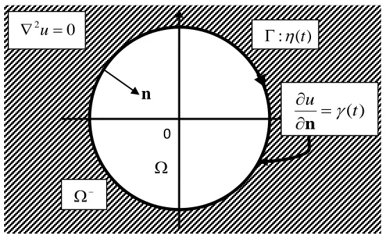
t t d . (3.1)Find the function u harmonic in , Hölder continuous on and satisfies on the boundary condition (see Figure 3.1)
. ) ( ),
(
) (
t t
u t
n (3.2)
The function u is also required to satisfy the additional condition
. as
|) (| )
(z O z 1 z
u (3.3)
Lemma 3.1(Atkinson, 1997)
Figure 3.1: The exterior Neumann Problem
3.2.1 Definition of Normal Derivative
The complex unit tangent vector T(t) is defined by
| ) ( |
) ( ) (
t t t
T
, (3.4)
where (t) is a complex parametrization of . We call T(t) the tangent directional derivative to at (t). We define the unit normal vector n to the curve at t to be the vector that is perpendicular to T(t) and has the same direction as T(t). By rotating the tangent T clockwise by
2
, we obtain
| ) ( |
) ( |
) ( |
) (
2
t t i t
t e i
n .
(3.5)
The directional derivative of u(x,y) in the direction of the outward unit normal to the path at point (t) is denoted by
n n
u u
, (3.6)
) ( : t
n
0
) (t u n
0
2
where u(x.y)uxiuyj. If (t)x(t)iy(t) is the parametrization of , then ) ( ) ( )
(t xt iyt
. Therefore, (3.5) becomes
j i j t t x i t t y t t y i t x i y x
n n
n
| ) ( | ) ( | ) ( | ) ( | ) ( | )) ( ) ( (
. (3.7)
Substituting (3.7) into (3.6), we obtain
| ) ( | ) ( ) ( t t x u t y u
u x y
n . (3.8)
3.2.2 The Exterior Riemann-Hilbert (RH) Problem
Definition 3.2 (Zamzamir et al.,2009)
The Exterior RH Problem. Given functions A and C, it is required to find a function g analytic in and continuous on the closure with g()0 such that the boundary values g satisfy ) ( ), ( ))] ( ( ) (
Re[At g t C t t . (3.9)
The boundary condition (3.9) can be written in the equivalent form
. ) ( , ) ( ) ( 2 )) ( ( ) ( ) ( )) ( ( t t A t C t g t A t A t
g (3.10)
. ) ( ,
0 ))] ( ( ) (
Re[At g t t (3.11)
The solvability of the RH problem is determined by the index
of the function A. The index of the function A is defined as the winding number of A with respect to zero. If the function A(t) is continuously differentiable on , then
dt
t A
t A i t
A d i A
) (
) ( 2
1 ) ( ln 2
1 ) (
ind
. (3.12)
The number of arbitrary real constants in the solutions of the homogenous RH problems, i.e. dim(S) and the number of conditions on the function C so that the non-homogenous RH problems are solvable, i.e. codim(R) are given in term of the index
as in the following theorem from Wegmann et al. (2005).Theorem 3.1.
The codimensions of the spaces R and the dimensions of the spaces S are given by the formulas
. ) 1 2 , 0 max( )
dim(
), 1 2 , 0 max( )
( codim
3.2.3 Integral Operators
Let A(t) be a continuously differentiable 2 periodicfunction with A0. We define two real functions N and M by
. ) ( ) ( ) ( ) ( ) ( Re 1 : ) , ( , ) ( ) ( ) ( ) ( ) ( Im 1 : ) , ( t t t A A t M t t t A A t N
We also define the kernels U and V (when A1 for the kernels N and M ) as
. ) ( ) ( ) ( Re 1 : ) , ( , ) ( ) ( ) ( Im 1 : ) , ( t t t U t t t V
We then define the kernels *
U and *
V (the adjoint kernels of U and V ) as
Lemma 3.2 (Wegmann et al., 2005).
(a) The kernel N(,t) is continuous with
) ( ) ( ) ( ) ( 2 1 Im 1 ) , ( t A t A t t t N .
(b) The kernel M(,t) has representation ( , ) 2 cot 2 1 ) ,
( M1 t
t t
M
with a continuous
kernel M1 which takes on the diagonal the values
) ( ) ( ) ( ) ( 2 1 Re 1 : ) , ( 1 t A t A t t t M .
3.2.4 Integral Equation for the Exterior Riemann-Hilbert Problem
For a given function C,H, let the function (z) be defined by . , ) ( ) ( ) ( 2 1 ) (
z z d A i C i z (3.13)
Based on the application of Plemelj‟s formula, a boundary integral equation with generalized Neumann kernel has been derived for exterior RH problem by Wegmann et al. (2005), as in the following theorem.
Theorem 3.2
If g(z) is a solution of the exterior problem (3.9) with boundary values
) ( ) ( )) ( ( )
(t g t C t i t
A (3.14)
. C M
N
(3.15)
By Theorem 3.2, if g((t)) is the solution of the exterior Riemann-Hilbert problem with boundary values
), ( ) ( )) ( ( )
(t g t t i t
(3.16)
then the imaginary part in (3.16) satisfies the integral equation
,
N M (3.17)
i.e.
. ) ( ) , ( )
( ) , ( )
(
2
0 2
0
N t t dt M t t dt (3.18)
The next theorem represents the solvability of the integral equation (3.15).
Theorem 3.3 (Zamzamir et al., 2009)
3.3 Modification of the Exterior Neumann Problem
3.3.1 Reduction of the Exterior Neumann Problem to the RH Problem
Suppose that u is the solution of the exterior Neumann problem and v is a harmonic conjugate of u in . The function f(z)u(x,y)iv(x,y) is analytic in where
j t y i t x t iy t x
t) ( ) ( ) ( ) ( ) (
:
if and only if the partial derivatives of u and v are continuous and satisfy the Cauchy-Riemann equations. The directional derivative of f in the direction of the outer unit normal vector to the path is given by
) ( )
(
) (
t t
v i u f
n n
n . (3.19)
Using the concept of normal derivative and Cauchy-Riemann equation, we obtain
) ( )
(
) )(
( )
(
t y x t
i f
f
n n
n
. (3.20)
Therefore, we can write (3.2) as the real part of (3.20),
) ( ] ) (
) ( Re[
)
( t
i f
t y
x
n n . (3.21)
Substituting (3.7) and (3.5) into (3.21), we get
( ) ( ).) (
) ( Re )
( Re
)
( t f t
t i f
t
n (3.22)
) ( ))] ( ( ) (
Re[ t g t t (3.23) which is the exterior RH problem as defined in Section 3.2.2. Comparison of (3.23) with (3.9) yields A(t)(t) and C(t)(t).
By Theorem 3.2, if g(z) is a solution of the exterior problem (3.23) with boundary values (t)g((t))(t)i(t), then the imaginary part satisfies the integral equation
N M . (3.24)
Applying (3.12) with A(t)(t), we obtain 1. From Theorem 3.1, we obtain
0 )
codim(R- which means that the non-homogenous exterior RH problem is solvable and 1
)
dim(S implies that the solution of the exterior RH problem is not unique. Also from Theorem 3.3, we conclude that the integral equation (3.24) is non-uniquely solvable. The approach to overcome the non-uniqueness is discussed in the following section.
3.3.2 Modified Integral Equation for the Exterior RH Problem
With A(t)(t), the kernel N becomes N(,t)V*(,t) while the kernel M becomes M(,t)U*(,t). Therefore, the non-uniquely solvable integral equation (3.24) become
* *
U V
. (3.25)
Recall from Section 3.1 that the function f is analytic on . Then at each point z
33
2 2 1
) (
z c z c z c z
f (3.26)
Differentiate once respect to z and multiply with iz, we obtain
) ( 3
2 )
( 33
2 2 1
z F z
c z
c z c z f
zi
(3.27)
Therefore,
z z F t
g(( )) ( ) since g((t))if((t)). By means of Cauchy Integral Formula, we obtain
. 0 ) (
d
g (3.28)
Notice that,
) (
) ( ) ( )) ( (
t t i t t
g
, so (3.28) becomes
. 0 ) ( )
(
2
0 2
0
t dt i t dt (3.29)Note that, the exterior Neumann problem need to satisfy (3.1). With (t)(t)(t) , (3.1) becomes ( ) 0
2
0
t dt which is the additional condition for the exterior RH problem which theright-hand side of the RH problem needs to satisfy. Thus (3.29) becomes
0 ) (
2
0
t dt . (3.30)Let the kernel (,t) be defined as
2 1 ) ,
2 0 2 0 ) ( 2 1 ) ( ) , ( )(t t t dt t dt
J . (3.31)
Therefore, we can write (3.30) as (3.31) where ( ) 0 2 1 ) ( 2 0
t t dt
J . Adding this integral equation with our integral equation (3.25) yields the new integral equation
* * U J
V
. (3.32)
According to Mikhlin (1957), this new integral equation (3.32) is uniquely solvable. The proof of the solvability of the integral equation can be followed from the paper written by Atkinson (1967).
From Lemma 3.2, we can write the kernel of the right-hand side of (3.32) as ) , ( ) , ( * t M t
U
which is singular since it is unbounded when t. To remove the difficulty, we will use the function B(,t) defined in Wegmann et al. (2005), with A(t)(t) where . for , ) ( ) ( Re ) ( ) ( 1 , for , ) ( ) ( ) ( ) ( ) ( ) ( Re 1 ) , ( t t t t t t t t t B (3.33)
Therefore, our uniquely solvable integral equation (3.32) becomes
V* J B (3.34)
where ( , ) .
2
0
B t dt
By obtaining , the Cauchy integral formula implies that the function f(z) can be calculated for z by
20 ( )
) ( ) ( ) ( ) ( 2 1 ) ( 2 1 ) ( z t dt t t i t i t i d z f i z
f (3.35)
and the function f(z) can be expressed as an anti-derivative function of f(z) for z. So we have . ) ( ) ( 1 log ) ( ) ( ) ( 2 1 ) ( 2 0 dt t z t t i t i t i z
f
(3.36)
3.4 Numerical Implementations of the Boundary Integral Equation
Since the function A(t)(t) and (t) are 2 periodic, the integrals in the integral equation (3.34) can be best discretized by the Nyström method with the trapezoidal rule as the quadrature rule (Atkinson, 1997). Let n be a given integer and define the n equidistant collocation points tk by
. , , 2 , 1 , 2 ) 1
( k n
n k
tk (3.37)
Then, using the Nyström method with the trapezoidal rule to discretized the integral equation (3.34), we obtain the linear system
n k nk j k
k n k j k n k j n k j
n B t t
n t t t J n t t t V n t 1 1 1 ) , ( 2 ) ( ) , ( 2 ) ( ) , ( * 2 ) (
(3.38)