Relationship between global stock exchanges and Indian stock market

28

Relationship between global stock exchanges and Indian stock market

Manas Mayur

Assistant Professor; Goa Institute of Management Sanquelim, Goa, India manasmayur@gim.ac.in

ARTICLE HISTORY:

Received: 07-Feb-2017

Accepted: 10-Mar-2017

Online available: 25-Mar-2017

Keywords:

Indian stock market, Integration,

Global stock market, Global cues

ABSTRACT

The Indian capital market has been always a subject of curiosity and research. Extensive research has been conducted over the years to predict the index, arguably till date no model could closely predict the index. It is also observed that the Indian stock market follows global cues which partially decide its direction for the day’s trading. Considering this fact, an attempt is made to study the global markets, to establish a mathematical model for forecasting the value of S&P BSE Sensex. The study employs a multiple regression model on daily stock prices of S&P BSE Sensex and few major global stock indices that would help an average investor to make an informed investment decision in Indian stock markets. It would act as a base for investors to take long term positions on the stocks traded on the exchange. The model would also help the policy makers to review key policy decisions based on global cues.

Contribution/ Originality

I declare and warrants that my contribution is original, except for such excerpts from copyrighted works as may be included with the permission of the copyright holder and author thereof, that it contains no libellous statements, and does not infringe on any copyright, trademark, patent, statutory right, or propriety right of others. The Author signs for and accepts responsibility for releasing this material on behalf of any and all co-authors.

DOI: 10.18488/journal.1007/2017.7.2/1007.2.28.41 ISSN (P): 2306-983X, ISSN (E): 2224-4425

Citation: Manas Mayur (2017). Relationship between global stock exchanges and Indian stock market. Asian Journal of Empirical Research, 7(2), 28-41.

© 2017 Asian Economic and Social Society. All rights reserved

Asian Journal of Empirical Research

Volume 7, Issue 2(2017): 28-41

29

1. INTRODUCTION

In 21st century, India; the country with vast land resources, the largest young population, ever growing energy needs, food, security and shelter; is poised to become the next global powerhouse. No matter the issues like political paralysis, crony capitalism and judicial adventurism continue to hurdle the economy. The growth is inevitable. The Indian Stock Market has been certainly a good barometer of the country’s economic health and aspirations for the last two decades. The fact remains, Indian growth story cannot be scripted alone in today’s world of globalisation. With elements of digitisation and mechanisation, with each passing day, the integration of the Indian stock market in global markets is growing steadily. The fact implies that the global markets are imminent source of information which cannot be ignored.

The Indian stock markets are a prime source of funds for the profit making institutions in the country. If the Indian economy is healthy and growing, it will reflect in the upward movement of stock prices, resulting in overall increase in stock market capitalisation. The total global invested share capital is Limited. Therefore, an increase in investment has to come from savings. To capitalise on stock arbitrage opportunities, one needs to give attention to: whether the overall global economy is expanding or declining or is stable? And what is the proportion of the fictitious economy/ unregulated economy in the global economy. These questions are also relevant to the Indian economy.

Now let’s assume that overall world economy is declining in FY2014-15. This is evident from the current low demand for oil, metals, EU crisis, unrest in West Asia, declining Chinese economy etc. On the other hand, if the Indian economy is growing or poised for growth as evident from the current levels of Indian Stock index S&P BSE Sensex, it only means that either domestic savings or foreign funds are infused in the Indian stock market. Now if I analyse the same on the pretext of a well-integrated global stock market, it means that the Indian stock index is performing better than the other comparable prominent global indices and not necessarily “overvalued”. The factors like people’s aspirations, political stability, strong economic fundamentals, etc. come into picture. This calls for proper study of markets to cash in the right time for investment, factor of safety and the right time to exit.

The objective of this study is to arrive at a mathematical model to establish the relationship between Indian stock index S&P BSE Sensex and major global stock indices. The model will provide an average investor, a systematic approach, based on statistical methods, to predict the value of S&P BSE Sensex based on global stock indices. The study would a measurement yard stick in the hands of investors to gauge the opportunities available at their doorsteps. The macro objective would be to make them aware about conditions suitable for investment and risk associated with it. Self-reliance and knowledge would promote more participation from retail investors for trading in stocks, which would ultimately build corpus to fuel economic growth in the country.

The scope of this study is limited to the collection of secondary data, analyse and present a mathematical model for prediction of future values of S&P BSE Sensex. The average daily closing stock prices for the various prominent global stock indices is collected. The datum is screened and analysed using statistical Methods using 95% confidence interval. The best fit statistical model is employed to arrive at a near perfect solution for sufficiently large number of observations. The analysis results are analysed for a test of significance and statistical errors. The best fit model is arrived which explains the relationship between S&P BSE Sensex and other selective global indices which impact the result. Finally the results are discussed and detailed conclusion of the study is presented for implementation and future studies.

30

S&P BSE Sensex index is overvalued or undervalued or stable. For policy makers, it would act as a guideline for deciding the economic policies for the country. For central bank of India (RBI), it will help in maintaining the optimum flow of money in the country for a healthy economy. For stock traders it would Suffice a base from where further micro level studies can be carried out to accurately predict the index.

2. LITERATURE REVIEW

Many studies have been conducted in the past to establish the empirical relationship between macro-economic variables and the stock index, causal effect analysis, impact of global stock indices etc.

Kumar and Singh (1998) conducted his study in the Indian market and observed that the joint impact of trading volume. Rate of exchange and the rate of the gold standard was highly significant on Sensex. The individual effect of rate of exchange and rate of the gold standard on Sensex was also found highly significant But the individual effect of trading volume was not found significant.

Raju and Ghosh (2004) observed that India experienced low intra-day volatility when compared to emerging markets and some of the developed markets. The extreme value volatility in India touched its Peak in 2000 and continuously decreased thereafter. Chattopadhyay and Behera (2005) found that the Indian stock market is not at all integrated with the world markets. Except short-term sentiment in the world market, the Indian stock market is not influenced by other markets.

Mukherjee (2007) made comparative analysis of Indian stock market with International Markets and observed that the markets do react to global cues, the Indian stock market is more integrated with other Global exchanges from 2002-03 onwards and that any major happening in the global scenario be it macro-economic or country specific affect the various markets. Raj and Dhal (2008) observed that within Asia, the Singapore and Hong Kong markets have significant influence, while the Japanese market has weak influence on the Indian market. The two global markets, the United States and the United Kingdom, have a differential impact on the Indian market in the opposite direction, amid a structural shift in India’s Integration with these global markets.

Singh and Sharma (2010) studied the inter-linkages between stock exchanges of BRIC nations and observed that the Indian stock exchange show a visible impact on the Brazilian and Russian stock exchange but not the Chinese stock exchange. Srikanth and Aparna (2012) observed that Sensex has a strong association with NYSE, Hang Seng and SSE Composite Index and a poor integration with NASDAQ and Nikkei225.

Chand and Thenmozhi (2012) found that global cues model significantly outperformed 1) past lags model and 2) technical indicators model used to predict in global markets. The analysis results suggest that most recent market information is more productive than the aged data. Study testaments that stock markets across the globe are integrated and that information on price transmissions can induce arbitrage opportunities. Thomas (2013) observed that the Indian capital market has undergone metamorphic reforms in the past five years. Every segment of the Indian Capital Market, namely, primary and secondary markets, derivatives, institutional investment, and market intermediation has experienced an impact of these changes, which has significantly improved the transparency, efficiency, and integration of the Indian market with the global markets. Kumarasamy (2013) concentrated on major informational efficiency and found with the help from many statistical tools that Indian IT stocks neither follows a random walk Nor weak from efficient.

31

3. METHODOLOGY

Data is collected from major global stock exchanges for daily adjusted closing prices. The sample indices selected for analysis represent all the major stock exchanges globally. The study attempts to establish the relationship between global Stock exchanges and the major Indian Stock exchange S&P BSE Sensex, to Establish a model to predict the Indian stock market.

I refer to previous studies conducted on the subject and I found that the Indian stock market is well integrated with the global stock markets, I verified the same and found a very high correlation of S&P BSE Sensex index with global stock indices.

In order to establish a near perfect model, I have made following logical assumptions.

i) Due to the high level of integration with global markets, if assume that the Indian stock market follows global market cues which decide on an average its direction for day trading session.

ii) Since some stock exchanges open prior to Indian stock exchange and others open after, it is appropriate to consider closing values of western stock exchanges a day preceding today.

The Table 1 below shows the sample list of major global stock exchanges selected for analysis. Table 1: Sample list of major global stock exchanges

Stock Exchange Opening Time (IST)

NYSE New York Stock Exchange 08.30 pm

TSE Tokyo Stock Exchange 05.50 am

LSE London Stock Exchange 01.30 pm

HKE Hong Kong Stock Exchange 07.55 am

BSE Bombay Stock Exchange 09.00 am

ASX Australian Securities Exchange 04.30 am

FWB Frankfurt Stock Exchange 01.30 pm

SSE Shanghai Stock Exchange 7.30 am

TSX Toronto Stock Exchange 08.00 pm

The daily adjusted closing prices of above mentioned stock exchanges are obtained from the yahoo finance website for the period from 07-07-1997 to 27-10-2014. The data are analysed after adjusting for non-working days in the respective stock exchanges and comparing all stock exchanges at par with S&P BSE Sensex after adjusting the closing prices for western stock exchanges. The data are analysed to establish a multiple regression model to predict future values of S&P BSE Sensex to given values of other prominent global stock exchanges.

Figure 1: Comparative time plot for global stock indices 0

5000 10000 15000 20000 25000 30000 35000

CAC 40

FTSE 100

HK Hang Seng

KOSPI Composite

NASDAQ

Nikkei 225

32

Upon analysing Fig 1, it is evident that stock movement has been stable since mid-year 2009 and makes sense to fit a regression line through this period to forecast future values. The period from 01/09/2009 to 27/10/2014 is selected for further analysis.

Following regression model is used for the analysis.

time t ASX of value X TSX of value X P S of value X Nekkei of value X index Composite NASDAQ of value X index Composite Kospi of value X Seng Hang HongKong of value X FTSE of value X CAC of value X Sensex BSE of value predicted Y Where X X X X X X X X X Y ASX TSX P S Nekkei NASDAQ Kospi Hangseng FTSE CAC Sensex t ASX t TSX t P S t Nekkei t NASDAQ t Kospi t Hangseng t FTSE t CAC t Sensex t                       200 500 500 & 225 100 40 200 500 500 & 225 100 40 ) ( 200 ) ( 9 500 ) ( 8 500 & ) ( 7 225 ) ( 6 ) ( 5 ) ( 4 ) ( 3 100 ) ( 2 40 ) ( 1 0 ) (            Sensex ASX Sensex TSX Sensex P S Sensex Nekkei Sensex NASDAQ Sensex Kospi Sensex Hangseng Sensex FTSE Sensex CAC Sensex Sensex

Y

in

error

random

const

iables

t

independen

other

holding

X

with

Y

of

Slope

const

iables

t

independen

other

holding

X

with

Y

of

Slope

const

iables

t

independen

other

holding

X

with

Y

of

Slope

const

iables

t

independen

other

holding

X

with

Y

of

Slope

const

iables

t

independen

other

holding

X

with

Y

of

Slope

const

iables

t

independen

other

holding

X

with

Y

of

Slope

const

iables

t

independen

other

holding

X

with

Y

of

Slope

const

iables

t

independen

other

holding

X

with

Y

of

Slope

const

iables

t

independen

other

holding

X

with

Y

of

Slope

ecept

Y













































.

var

,

.

var

,

.

var

,

.

var

,

.

var

,

.

var

,

.

var

,

.

var

,

.

var

,

int

200 9 500 8 500 & 7 225 6 5 4 3 100 2 40 1 0

To start with I conducted multiple regression analysis on all nine selected independent variables 40

CAC

X

_,

X

FTSE100_,

X

Hangseng_,

X

Kospi_,

X

NASDAQ_,

X

Nekkei225_,

X

S&P500_,

X

TSX500 _and

X

ASX200 with 95% confidence interval. From the ANOVA Summary table, I found

p



value

for three independent variables

X

NASDAQ,

X

Nekkei225 _and

X

ASX200_{greater than significance value α=0.05.} Hence the three variables are rejected and the mathematical function is reframed as below.

) ( 500 ) ( 6 500 & ) ( 5 ) ( 4 ) ( 3 100 ) ( 2 40 ) ( 1 0 )

(tSensex XtCAC XtFTSE XtHangseng XtKospi XtS P XtTSX t

33

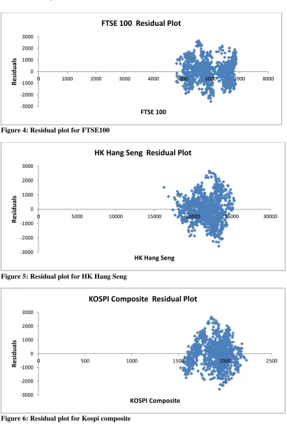
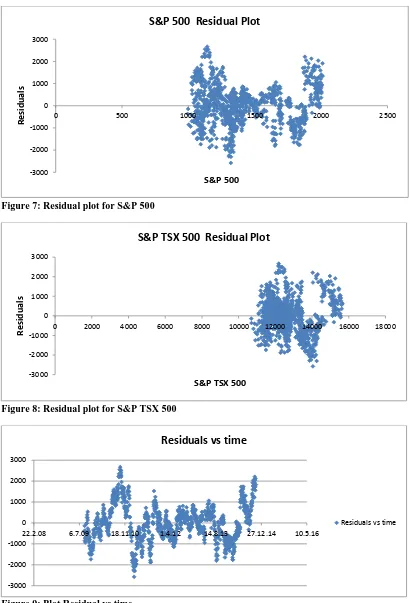
The following residual plots were constructed To evaluate the appropriateness of multiple regression model.

i) Residuals verses

Y

Sensex

ii) Residuals verses each independent variables 40

CAC

X

,

X

FTSE100_,

X

Hangseng_,

X

Kospi_,

X

S&P500_,

X

TSX500 iii) Residuals verses time

Figure 2: Plot for Residuals vs Predicted values of S&P BSE Sensex

Figure 3: Residual plot for CAC40 -3000

-2000 -1000 0 1000 2000 3000

0 5000 10000 15000 20000 25000 30000

Residuals vs Predicted S&P BSE Sensex

Residuals

-3000 -2000 -1000 0 1000 2000 3000

0 500 1000 1500 2000 2500 3000 3500 4000 4500 5000

R

e

si

d

u

al

s

CAC 40

34 Figure 4: Residual plot for FTSE100

Figure 5: Residual plot for HK Hang Seng

Figure 6: Residual plot for Kospi composite -3000

-2000 -1000 0 1000 2000 3000

0 1000 2000 3000 4000 5000 6000 7000 8000

R

e

si

d

u

al

s

FTSE 100

FTSE 100 Residual Plot

-3000 -2000 -1000 0 1000 2000 3000

0 5000 10000 15000 20000 25000 30000

R

e

si

d

u

al

s

HK Hang Seng

HK Hang Seng Residual Plot

-3000 -2000 -1000 0 1000 2000 3000

0 500 1000 1500 2000 2500

R

e

si

d

u

als

KOSPI Composite

35 Figure 7: Residual plot for S&P 500

Figure 8: Residual plot for S&P TSX 500

Figure 9: Plot Residual vs time -3000

-2000 -1000 0 1000 2000 3000

0 500 1000 1500 2000 2500

R

e

si

d

u

al

s

S&P 500

S&P 500 Residual Plot

-3000 -2000 -1000 0 1000 2000 3000

0 2000 4000 6000 8000 10000 12000 14000 16000 18000

R

e

si

d

u

al

s

S&P TSX 500

S&P TSX 500 Residual Plot

-3000 -2000 -1000 0 1000 2000 3000

22.2.08 6.7.09 18.11.10 1.4.12 14.8.13 27.12.14 10.5.16

Residuals vs time

36 Upon analysing the above plots I note the following:

1) There is no pattern observed in the plots except the residual vs time plot.

2) The plot, residuals vs time, is used to investigate patterns in the residuals in order to validate the independence assumption. For this the data need to be collected in time order. Upon analysing the plot, I observe a cyclical pattern in the values of residuals w.r.t. time. The Durbin-Watson statistic was used to Determine the existence of positive autocorrelation among the residuals. For significance level α= 0.05, the sample size n= 1083 and the number of independent variables in the model k=6, I find Durbin-Watson statistic D= 0.084465. From Table A.2 for critical values of the Durbin-Watson statistic

d

L =~1.56 and

d

U_{=~1.8, I find D<}

d

L _{(approaching to zero) which means that there is} presence of significant positive autocorrelation among the residuals (independence of errors assumption is invalid). The remedial measure taken to address this issue is explained in the next sub section below in detail.

3) To evaluate the assumption of normality of the errors, I plot the normality plot for residuals. I observe that the data do not appear to depart substantially from a normal distribution. The regression analysis is fairly robust and since the errors at each level of X is not extremely different from a normal distribution. Inferences about β coefficients are not seriously affected.

This concludes that the multiple regression model is appropriate for predicting value of S&P BSE Sensex. If I did not find any pattern in the plot, it indicates that there is no existence of quadratic effect and therefore no need to add a quadratic independent variable to the multiple regression model.

Remedial measures for Autocorrelation

The two principal remedial measures when auto correlated error terms are present are to add one or more predictor variables to the regression model or to use transformed variables.

I used a transformation of variables method to eliminate the problem of auto correlated errors. The new fitted regression function with transformed variables is as follows:

where u X X X X X X

Y tSensex  tCAC  tFTSE  tHangseng tKospi tS P  (t)TSX500 t

37 terms e disturbanc t independen the are u the e e u term error Y in error random of value d transforme parameter ation autocorrel value t iable t independen original X value t iable t independen original X value t iable t independen for iable d transforme X value t Sensex BSE of value predicted for iable original Y value t Sensex BSE of value predicted for iable original Y value t Sensex BSE of value predicted for iable d transforme Y Where t t t t Sensex th t th t th t th Sensex t th Sensex t th Sensex t , , ) 1 ( var var var var ) 1 ( var var var ) 1 ( ' ) 1 ( ) ( ) ( ' ) 1 ( ) ( ) ( ' 6 6 ' 3 3 ' 2 2 ' 1 1 '                      



























Thus, by using the transformed variables

Y

(t)Sensex

'

and () '

t

X

_{, I obtain a standard linear regression}

model with Independent error terms. This also means that the usual optimum properties of ordinary least squares methods would be applicable for this transformed model.

To use the above shown transformed model, I need to have an estimate of the autocorrelation parameter



, its value is currently unknown. I use the Cochrane- Orcutt procedure for estimating the autocorrelation parameter. The procedure involves an iteration of three steps shown below.

1) Estimation of



: I understand that the autoregressive error process assumed in above model is simply a Regression through the origin. Therefore I have,



t





(t1)



u

t

where



t_{is the response variable,}



(t1)_{the predictor variable,}

u

t_{the error term and the}



slope of the line through the origin. I use the residuals

e

t_and

e

t1_{obtained from the original} multiple regression model instead of unknowns



t_and



(t1)_{. Then I obtained estimate of}



_{(the slope of the straight line through the origin) as per equation shown below.}





     _n t t n t t t e e e 2 ) 1 ( 2 2 ) ( ) 1 ( 

2) Fitting of the transformed model: I next obtain the transformed variables

Y

(t)Sensex

' and ) ( ' t

38

least squares method with these transformed variables. The resulting output obtained is the ANOVA table with



estimates and residuals.

3) Test for positive autocorrelation: The Durbin-Watson test statistic obtained from the regression analysis is used to test whether the error terms for the transformed multiple regression model are uncorrelated. If the test indicates that error terms are uncorrelated, the Cochrane- Orcutt procedure terminates. I transform The regression coefficients back to its fitted regression model with original variables.

4) If the Durbin-Watson test indicates that in the first iteration autocorrelation is present, the parameter



is re-estimated from the new residuals for the fitted regression model with the original variables, which are derived from the transformed regression model. The process continues with the next iteration until the error terms of the transformed model are uncorrelated. If error terms are still correlated after two iterations, the procedure is discontinued and new methodology to be adopted.

I used the above methodology to eliminate the autocorrelation present in residuals. I obtained the autocorrelation parameter



=0.9595. Upon running multiple regression analysis with transformed variables, I found Durbin-Watson test statistic D= 1.89347, for the number of observations n= 1082, number of independent variables with k=6 and level of significance α=0.05. From the table A.2- critical values

d

L_and

d

U_{the Durbin-Watson statistic; I note as n increases,}

d

L_and

d

U_decreases. Since D=1.89347 is greater than the

d

U_{, I statistically conclude that there is no evidence of} autocorrelation among the residuals of transformed regression function. The Cochrane- Orcutt procedure is terminated at its 1st iteration.

I obtained the value of transformed regression coefficients shown below:

Coefficients Value

Intercept 298.86

CAC 40 -0.40

FTSE 100 -0.31

HANGSENG 0.34

KOSPI 1.06

S&P 500 4.74

TSX 500 -0.07

I transformed regression coefficients back to its fitted regression model with original variables. The resulting original regression coefficients are shown below.

Coefficients Value

Intercept 7,382.62

CAC 40 -0.40

FTSE 100 -0.31

HANGSENG 0.34

KOSPI 1.06

S&P 500 4.74

TSX 500 -0.07

39

t t TSX

t P

S t

Kospi t Hangseng

t FTSE

t CAC

t Sensex

t

u

X

X

X

X

X

X

Y

























1) ( 500 ) ( 500

& ) (

) ( )

( 100

) ( 40

) ( )

(

)

07

.

0

(

74

.

4

06

.

1

34

.

0

)

31

.

0

(

)

40

.

0

(

62

.

7382



4. RESULTS AND DISCUSSION

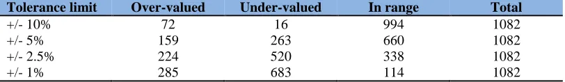
Using the above mathematical model established through statistical methods, I compared the predicted values of S&P BSE Sensex verse the actual values of S&P BSE Sensex. The % difference between actual v/s predicted values were taken and categorised into three conditions shown below.

i) OVER-VALUED: The instance wherein the % difference is greater than the set upper tolerance Limit. This implies that the Indian stock index is overvalued w.r.t. the pool of global stock indices.

ii) UNDER-VALUED: The instance wherein the % difference is lesser than the set lower tolerance Limit. This implies that the Indian stock index is undervalued w.r.t. the pool of global stock indices.

iii) IN RANGE: The instance wherein the % difference is in between the set tolerance Limits This implies that the Indian stock index is in line w.r.t. the pool of global stock indices.

I have evaluated the result based on the four cases shown below.

Tolerance limit Over-valued Under-valued In range Total

+/- 10% 72 16 994 1082

+/- 5% 159 263 660 1082

+/- 2.5% 224 520 338 1082

+/- 1% 285 683 114 1082

For daily stock traders, if I examine the result with +/- 1% tolerance limit, the result indicates that almost 63% of the instances are such that the S&P BSE Sensex index is undervalued w.r.t the pool of global stock indices. The investors have an opportunity and may cash in to buy stocks during this period with a long term perspective provided the economic health of the country is good and growth oriented. This may not be true most of the times hence one need to be cautious.

For policy makers, if I examine with +/-10% tolerance limit, an overvalued result certainly mean Indian economy is doing much better than the global economy, the result to be seen in association with other economic indicators like political stability, FII, DII inflows, GDP, IIP and exchange rate fluctuations. An Undervalued result may indicate weaker Indian economic status but the elements of fictitious/unregulated economy may contribute to marginally hold and give strength to the economy. The overvalued status of the Indian stock market may need not always mean highly cautious or peak position inhibiting further investment. For example, if the FIIs and DIIs inflow is much higher than expected during this period, it means that the current economic condition of India (includes future aspirations) is Much stronger than rest of the world.

Let’s look at the monthly average % difference between actual v/s predicted values of S&P BSE Sensex for the last 5 years.

Table 2: % Difference between actual and predicted value of S&P BSE Sensex (monthly average)

Month-Year Average per month Month-Year Average per month

Oct-14 10.7% Mar-12 -7.0%

Sep-14 12.3% Feb-12 -6.3%

40

Jul-14 11.7% Dec-11 -9.8%

Jun-14 9.5% Nov-11 -6.9%

May-14 6.9% Oct-11 -8.6%

Apr-14 7.4% Sep-11 -2.2%

Mar-14 6.9% Aug-11 -1.6%

Feb-14 4.9% Jul-11 -4.0%

Jan-14 3.8% Jun-11 -2.3%

Dec-13 2.9% May-11 0.0%

Nov-13 1.1% Apr-11 2.7%

Oct-13 -1.5% Mar-11 5.3%

Sep-13 -2.7% Feb-11 3.4%

Aug-13 -3.0% Jan-11 -0.9%

Jul-13 -4.0% Dec-10 0.4%

Jun-13 -5.0% Nov-10 0.8%

May-13 -5.0% Oct-10 -0.7%

Apr-13 -5.5% Sep-10 -3.1%

Mar-13 -4.3% Aug-10 -3.7%

Feb-13 -2.6% Jul-10 -4.0%

Jan-13 -1.8% Jun-10 -2.2%

Dec-12 -4.0% May-10 -1.0%

Nov-12 -3.0% Apr-10 -2.4%

Oct-12 -3.6% Mar-10 -2.2%

Sep-12 -6.3% Feb-10 -2.9%

Aug-12 -8.6% Jan-10 -2.4%

Jul-12 -8.0% Dec-09 -0.2%

Jun-12 -8.9% Nov-09 1.2%

May-12 -7.9% Oct-09 -1.2%

Apr-12 -7.2% Sep-09 -3.1%

From the above table, I note % difference steadily grows from Dec 2013 to Sept 2014. The economic status may be termed “overvalued”, however one may relate this to a period during which the national elections were fast approaching and I saw expected change in power at the center with the Bharatiya Janata Party (BJP) emerging victorious with a huge majority. With Mr. Narendra Modi swore in as Prime Minister in May 2014, the expectations of the people from the New Government have created a pro-economic environment, which has translated into “overvalued” status for the Indian stock market in w.r.t. global stock indices. The mathematical model apparently demonstrates correctly the true economic Status of the country during this period.

Further I note the period from Sept 2009 to Sept 2011, the post-recession period, the Indian economy showed signs of recovery. Table 2 above shows % difference in and around 0% and moves steadily in positive zone till May 2011 and then deteriorating again further into negative zone till Nov 2013. One may recall. This was the period during which I saw poor governance in the country. The judicial adventurism and Crony capitalism adding to the woes of the country with GDP dropped under 4.5%, marking a 10 years low. The mathematical model again demonstrates correctly the true economic status of the country during this period.

5. CONCLUSION

41

volatile and moves in a cyclical manner. This is true for both short term and long term trends. The short term movement, although volatile, is mostly within its range and this model would be able to suffice as it moves in a definite direction. But the sudden long term reversal in direction can be catastrophic and one needs to be careful to judge the sudden collapse. The above model can help to monitor the index and can alarm in such extreme cases. For an average investor, the above model, if used judiciously with other economic indicators, can be very helpful to reap huge returns/benefits from the Indian stock market for both long and short terms.

Funding: This study received no specific financial support.

Competing Interests: The author declares that s/he has no conflict of interests.

Contributors/Acknowledgement: All the designing and estimation of current research done by the sole author.

Views and opinions expressed in this study are the views and opinions of the authors, Asian Journal of Empirical Research shall not be responsible or answerable for any loss, damage or liability etc. caused in relation to/arising out of the use of the content.

References

Chand, G., & Thenmozhi, M. (2012). Do Global stock market cues matter in forecasting stock returns in developed and developing markets?. Dept. of Management studies, IIT Madras.

view at Google scholar

Chattopadhyay, S., & Behera S. (2005). Financial integration for Indian stock market. Dept. of economic analysis and policy of the Reserve Bank of India. view at Google scholar

Kumar, R., & Singh B. (1998). Impact of Trading Volume, Rate of Exchange (Dollar) and Gold Standard on Sensex. The Indian Journal of Commerce, 51(4), 19-27. view at Google scholar

Kumarasamy, U. (2013). Random walk in return on banking stocks-empirical evidence from India.

Global Management Review, 6(4), 21-43. view at Google scholar

Mukherjee, D. (2007). Comparative analysis of Indian stock market with international markets.

Great Lakes Herald, 1(1), 39-71. view at Google scholar

Raj, J., & Dhal, S. (2008). Integration of India’s stock market with global and major regional

markets. Press & Communications CH 4002 Basel, Switzerland, 202. view at Google scholar

Raju, M. T., & Ghosh, A. (2004). Stock Market Volatility–An International Comparison. Securities and Exchange Board of India. view at Google scholar

Srikanth, P., & Aparna, K. (2012). Global stock market integration-a study of select world major stock markets. Researchers World, 3(1), 203. view at Google scholar

Singh, S., & Sharma, G. D. (2012). Inter-linkages between stock exchanges: A study of BRIC nations. International Journal of Marketing, Financial Services and Management Research,

1(3), 1-17. view at Google scholar/ view at publisher