HIGHLIGHTED ARTICLE
| INVESTIGATION
Estimating Barriers to Gene Flow from Distorted
Isolation-by-Distance Patterns
Harald Ringbauer,*,1Alexander Kolesnikov,* David L. Field,†and Nicholas H. Barton*
*Institute of Science and Technology Austria, Klosterneuburg A-3400, Austria, and†Department of Botany and Biodiversity Research, University of Vienna, A-1030, Austria ORCID IDs: 0000-0002-4884-9682 (H.R.); 0000-0002-4014-8478 (D.L.F.); 0000-0002-8548-5240 (N.H.B.)
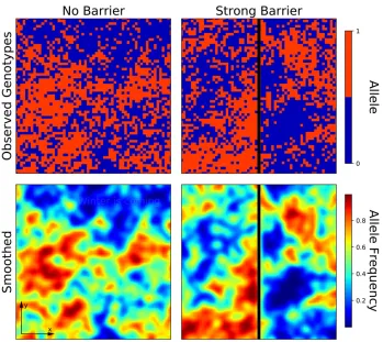
ABSTRACTIn continuous populations with local migration, nearby pairs of individuals have on average more similar genotypes than geographically well-separated pairs. A barrier to geneflow distorts this classical pattern of isolation by distance. Genetic similarity is decreased for sample pairs on different sides of the barrier and increased for pairs on the same side near the barrier. Here, we introduce an inference scheme that uses this signal to detect and estimate the strength of a linear barrier to geneflow in two dimensions. We use a diffusion approximation to model the effects of a barrier on the geographic spread of ancestry backward in time. This approach allows us to calculate the chance of recent coalescence and probability of identity by descent. We introduce an inference scheme that
fits these theoretical results to the geographic covariance structure of bialleleic genetic markers. It can estimate the strength of the barrier as well as several demographic parameters. We investigate the power of our inference scheme to detect barriers by applying it to a wide range of simulated data. We also showcase an example application to anAntirrhinum majus (snapdragon)flower-color hybrid zone, where we do not detect any signal of a strong genome-wide barrier to geneflow.
KEYWORDSbarriers to geneflow; isolation by distance; identity by descent; demographic inference
M
ANY populations are distributed across geographically extended habitats that are sometimes interrupted by barriers to geneflow. They can arise due to physical obstacles that reduce migration, but can also be caused by genetic incompati-bilities, which reduce geneflow across a hybrid zone (Barton 1979). Barriers can prevent locally adapted populations from being swamped by dispersal and they can facilitate divergence, ultimately leading to speciation. Therefore, they play a central role not only in conservation, but also in evolutionary biology and ecology. As direct observations of individual movement and re-production are time consuming, expensive, and can only give a snapshot in time, there is much interest in indirect methods that infer such barriers from observed geographic genetic structure.Such methods to detect barriers from genetic data can be grouped into two distinct approaches (Guillotet al.2009): clus-tering methods, which detect geographic genetic discontinuities
between populations by grouping individuals into population units based on genetic similarity (Dupanloup et al.2002; Falushet al.2003; Guillotet al.2005); and edge-detection methods, which identify areas of sharp genetic change (Womble 1951; Manniet al.2004; Cercueilet al.2007). Neither of these approaches is directly linked to any spatial population genetic model. They can therefore infer the existence of a barrier, but cannot give meaningful and biologically interpretable estimates of its strength. In addition, these approaches are often con-founded by isolation-by-distance patterns (Safneret al.2011; Meirmans 2012), whereby individuals nearby are more similar than distant individuals (Wright 1943) due to recent coan-cestry. While the description of this effect has a long history in theoretical population genetics of homogeneous popula-tions (Malécot 1948; Slatkin 1993; Rousset 1997; Hardy and Vekemans 1999; Bartonet al.2002), it has not been included into a practically applicable method to estimate the strength of a barrier to geneflow.
Here, wefill this gap and introduce a method that infers the strength of a barrier in a two-dimensional population byfitting a population genetic model. Our method uses the fact that a bar-rier to geneflow distorts classical isolation-by-distance patterns (Figure 1). Based on the theoretical work of Nagylaki (1988), Copyright © 2018 by the Genetics Society of America
doi:https://doi.org/10.1534/genetics.117.300638
Manuscript received October 19, 2017; accepted for publication December 23, 2017; published Early Online January 8, 2018.
Supplemental material is available online atwww.genetics.org/lookup/suppl/doi:10. 1534/genetics.117.300638/-/DC1.
1Corresponding author: Institute of Science and Technology Austria, Am Campus 1,
Barton (2008) constructed a theoretical framework. He showed that in two spatial dimensions, wherefluctuations of allele fre-quencies are more localized than in one dimension, these effects of a barrier on allele-frequencyfluctuations can already be sig-nificant for intermediate barrier strengths. This signal therefore has great potential for demographic inference. The derivation of Barton (2008) also shows that the effect of a barrier depends primarily on short-lived, localized fluctuations. In general, isolation-by-distance patterns equilibrate relatively quickly and depend mostly on recent demography (Barton et al.
2013; Aguillonet al.2017). Therefore, an inference scheme based on distorted isolation-by-distance patterns infers con-temporary barriers to geneflow, and should be robust to con-founding effects of ancestral structure.
Here, we first expand previous theoretical results that describe the effect of a barrier on classical isolation-by-dis-tance patterns (Nagylaki 1988; Barton 2008). We introduce a model where ancestry diffuses backward in time and is par-tially reflected by a barrier. This allows us to numerically calculate the probability of recent coancestry, which can then befitted to genetic data. As single nucleotide polymorphism (SNP) data sets are currently widely used, we develop and implement ways tofit such biallelic genetic markers.
We test our inference scheme on synthetic data simulated under an explicit population genetics model and investigate how it is affected by confounding factors, for instance in a scenario of secondary contact. We also show a practical application in which we apply our inference scheme to a hybrid zone population of
Antirrhinum majus, in which a sharp transition inflower color and a causalflower-color gene occurs (Whibleyet al.2006). We apply our method to test whether there is also a genome-wide barrier to contemporary geneflow. To this end, we analyze a data set of 12,389 individuals and 60 suitable SNP markers.
Materials and Methods
Wefirst outline the model underlying our inference scheme and discuss its assumptions, and then describe how our methodfits this model to observed genotype data. In brief, we use a diffusion approximation for the spread of ancestry to calculate the probability of recent identity by descent between pairs of samples. We thenfit our model to data byfinding the demographic parameters that maximize the fit of observed homozygosity between all sample pairs.
Model
No model can capture all complexities of the real demographic history of a population. Therefore, the aim is not to have a mathematically exact model, but one that robustly captures general patterns of spatialfluctuations of allele frequencies. We use a model of a two-dimensional continuous habitat that is interrupted by a barrier and assume that the demographic parameters are the same on both sides. In short, we calculate the chance of pairwise coalescence before a long-distance mi-gration or mutation event. We use a diffusion model to trace lineages backward in time and assume that rare long-distance
migration events, which counteract the buildup of local allele-frequencyfluctuations, occur at a constant rate. To calculate the equilibrium identity-by-descent pattern,i.e., the probability that two lineages coalesce before the occurrence of a rare long-dis-tance migration or mutation event, wefirst derive the coalescence probability at specific timestin the past and then integrate overt. Our model is closely related to previous theoretical treat-ments of allelic identity by state in presence of a barrier to gene
flow (Nagylaki 1988; Barton 2008). For a population occu-pying a linear habitat, Nagylaki (1988) derived continuous equations for identity by state by taking the limit of a model of linear demes that exchange migrants (the so-called stepping-stone model). Barton (2008) expanded this by solving an anal-ogous equation for two-dimensional populations. His formulas are given as a numerical Fourier transform that diverges for nearby individuals. These equations for two-dimensional pop-ulations are formally problematic as they were not obtained by rescaling (which is impossible in two spatial dimensions), but Barton (2008) demonstrated that the solution is in close agree-ment with the solutions from a discrete stepping-stone model for all but very close distances.
Here, we base our inference scheme on a different ap-proach. We use a diffusion approximation to describe the spread of ancestry backward in time. While the results are formally equivalent, we found our model to be computationally more robust and, most importantly, more efficient. This approach allows us to apply our method to sample sizes of hundreds to thousands of individuals, and dozens to hundreds of loci.
Diffusion approximation:We model the spread of ancestry
using a geographic diffusion approximation, which has a long history in population genetics (Fisher 1937; Wright 1943; Malécot 1948; Nagylaki 1978). Tracing a lineage of one locus backward in time, the total spatial movement is the sum of many independent migration events. If these events are
suf-ficiently uncorrelated, the central limit theorem establishes that the total displacement tends toward a normal distribu-tion. Therefore, the overall spread of ancestry can be approx-imated as a random walk process. This approximation is accurate as long as rare large-scale events do not significantly influence the movement of ancestral lineages. The diffusion approximation is expected to be most accurate on recent to intermediate timescales, on which large-scale events such as colonizations often play only a minor role.
In the absence of a barrier, the process is a free diffusion and the probability density function offinding an ancestor at posi-tionxat timetback along a given axis is given by a Gaussian probability density function around the current positionx0and variances2tthat increases linearly backward in time:
G0ðx;x0;tÞ:¼ ffiffiffiffiffiffiffiffiffiffiffiffiffi1
2ps2t
p exp 2ðx2x0Þ
2
2s2t !
: (1)
The dispersal rate s describes the speed of the spread of ancestry. In the case of a homogeneous density of individuals across the landscape, the backward dispersal probability
den-sity equals the probability denden-sity of lineages moving forward in time. In this particular case, the dispersal rate s2 can be interpreted as the axial variance of the one generational dis-persal kernel (Rousset 1997). The diffusion approximation is fully determined by the equation:
@
@tGðx;x0;tÞ ¼ s2
2
@2
@x2Gðx;x0;tÞ; (2)
with initial condition:
Gðx;x0;t¼0Þ ¼dðx2x0Þ: (3)
Partial barrier to geneflow:We model a barrier as a partially permeable barrier to diffusion of ancestry. For a barrier at
x¼0;the following interface boundary conditions have to be supplied (Grebenkovet al.2014):
lim e/0
@
@xGðx;x0;tÞ
x¼þe ¼ lim
e/0
@
@xGðx;x0;tÞ
x¼2e
¼2k
s2
lim
e/0Gðe;x0;tÞ2elim/0Gð2e;x0;tÞ
:
(4)
The first line describes the constancy of theflux across the barrier. Fork¼0;there is noflux across the barrier and the barrier is infinitely strong. On the other hand, the casek¼N
implies the continuity of the probability density across the barrier and the solution reduces to free diffusion. Comparing to the differential equation 54 in Nagylaki (1988), which is derived by rescaling a stepping-stone model, gives an intui-tive interpretation ofk: This parameter corresponds to the fraction of successful migrants across a barrier if demes are spaced one dispersal unit apart. The quotientg:¼2k
s2 corre-sponds to an equivalent factor in equation 54 of Nagylaki (1978). It is also the inverse of the barrier strength parameter
B defined by Barton and Bengtsson (1986), which has the dimension of distance.
Equations 2–4 allow for an analytic solution for the prob-ability density with a barrier (Grebenkovet al.2014):
Gðx;x0;tÞ ¼
exp 2ðx2x0Þ
2
2s2t !
þexp 2ðxþx0Þ
2
2s2t !
ffiffiffiffiffiffiffiffiffiffiffiffiffi 2ps2t
p 2
22k
s2exp
4k
s2ðx02xþ2kt
erfc
x02xþ4kt ffiffiffiffiffiffiffiffiffiffi 2s2t p
;x.0;
2k s2exp
4k
s2ðx02xþ2ktÞ
erfc
x02xþ4kt ffiffiffiffiffiffiffiffiffiffi 2s2t p
;x,0; 8 > > > > > > > > > > > > > > < > > > > > > > > > > > > > > : (5)
x;x0/2x;2x0: The transition density converges to the Gaussian of free Brownian motion fork/N:For a two-dimensional diffusion process with a linear barrier, the full transition density is obtained by multiplying the one-dimensional density functions from Equation 2 for movement parallel to the barrier with Equation 5 for movement orthogonal to the barrier.
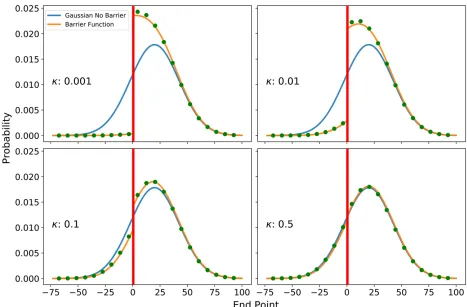
Forien (2017) showed that the one-dimensional transition density can be also obtained as a scaling limit of a one-dimensional discrete random walk with a partially reflective barrier. This result indicates that the continuous model is also a good ap-proximation for stepping-stone barrier models. We compared the continuous formula to discrete random walk simulations, and there is indeed close agreement (Figure 2).
Pairwise coalescent probabilities: We use the diffusion
ap-proximation to model the distribution of coalescence times for pairs of individuals. We approximate the chance of coancestry originating in a small time intervaldtaround timetago as the product of the probability of coming close and a rate of local coalescence 1=2De(Ringbaueret al.2017). The local density
De describes a rate with which nearby lineages coalesce (Wright 1943). In a stepping-stone model, De corresponds to the number of diploid individuals per deme (Bartonet al.
2002). This approximation ignores that lineages do not move apart again once they have coalesced. An equivalent
simpli-fication is made by Barton (2008), and it is accurate as long as coalescence is sufficiently rare (Wilkins 2004). Since the dis-persal process is symmetrical in time in our model of constant population density, the chance that two lineages at current positionp1andp2 are close at timetback equals the proba-bility density that a single lineage moves fromp1top2in time 2t: Formally, the probability density cðp1;p2;tÞ of coales-cenceTcat timetin the past is approximated by
cðp1;p2;tÞ ¼Pr
Tc2 ½t;tþdt
dt G
p1;p2;2t 1
2De: (6)
Empirical simulations for a stepping-stone model confirm that this model approximates the pairwise coalescence time dis-tribution on recent to intermediate timescales (Supplemental Material,File S1).
Identity by descent: We define identity by descentFof two samples atp1andp2as the chance that two lineages coalesce before a long-distance migration or, equivalently (but un-likely for SNPs), a mutation event occurs along one of the lineages. This definition is closely related to the widely used
Figure 2 Comparison of analytical diffusion formulas (Equation 4) with discrete random walk simulations fort¼500 in the past. We simulated a one-dimensional random walk on an array of linear discrete nodes at all integers and a barrier atx¼0:5:Every generation, a random step to one side is made (which implies thats¼1). If a movement would be across the barrier (red line), it is realized with probabilityk(otherwise no step is made). For each of four barrier strengths, we simulated 106replicates starting atx¼20:The blue line depicts the corresponding Gaussian probability density of
fixation indexFST;and both definitions agree in the limiting case of an infinite population (see Rousset 2002 for a review). If one assumes that mutation or long-distance migration occurs at a constant ratem, it is straightforward to calculate the probability that two lineages coalesce before a long-distance event:
Fðp1;p2Þ ¼ Z N
0
cðp1;p2;tÞexpð22mtÞdt: (7)
In the absence of a barrier, the probability of identity by descent depends only on the Euclidean distance between two individuals. In this special case, the integral in Equation 7 has an analytical solution, the classical Wright–Malécot formula (Bartonet al.2002, 2013):
FðrÞ ¼ 1
4pDes2K0 ffiffiffiffiffiffi
2m
p r
s
; (8)
whereK0is the modified Bessel function of the second kind of degree zero. A caveat of this analytical solution is that K0 diverges logarithmically asr/0 (Bartonet al.2002). Simi-larly, the integral in Equation 7 diverges for nearby individu-als. As for the Wright–Malécot formula, this is caused by a behavior of the diffusion approximation for short timescales, as the chance of two lineages being close diverges as 1=tfor
t/0:A solution to circumvent this problem is to start inte-gration at timet0.0:Here, we choose one generation time, a biologically plausible value. We could notfind an analytical solution, but Equation 7 can be numerically integrated.
Our calculations show that if a barrier to gene flow is present, identity is decreased across the barrier, and increased for points on the same side of the barrier (Figure 3). Inter-estingly, the increase ofFfor a pair of pointsp1andp2on the
same side of the barrier equals the decrease of F between pointsp1andp92;wherep92 is the reflection ofp2across the barrier. This symmetry originates from a reflection principle of the underlying random-walk model, as lineages that do not cross the barrier behave as if they were reflected. This sym-metry already occurs in the barrier point density function (Equation 5). It implies that, for a complete barrier, identity by descent can increase to at most twice of the value in ab-sence of a barrier, as observed in the equivalent case of a range boundary (Wilkins 2004).
As already noted by Barton (2008), a barrier to geneflow mostly affects recent coancestry, whereas deeper coalescence probabilities are not distorted much (File S1). In particular, weighted mean coalescence times for individuals from the same deme remain completely invariant in deme models with conservative migration (i.e., constant population density), in-dependent of the specific migration scheme (Nagylaki 1998; Laporte and Charlesworth 2002). We used models of this type in our simulations below to approximate our continuous spa-tial theory. However, this invariance of mean coalescence times is not problematic for our inference method. When calculating allele frequency correlations, pairwise coalescence probabili-ties are weighted by a factor expð22mtÞ;which accounts for rare, but nonnegligible long-distance migration events. It de-cays exponentially with time. Therefore, our method is based on a signal of mostly recent coalescence events. Reassuringly, this is also the timescale on which barriers affect pairwise co-alescence probabilities the most, and on which the spatial dif-fusion approximation is likely most accurate (File S1).
Rescaling:Not all parameters in Equation 7 are independent. Consequently, they cannot be estimated separately, as in
Figure 3 Decay of identity by descentFin presence of a strong barrier to geneflow (k¼0:01) and moderate neighborhood size (s¼1;De¼5;and
absence of a barrier (Rousset 1997; Barton et al. 2013). Therefore, we replace the four demographic parameters
u
!
:De;k;m;sin Equation 6 with three compound parame-tersu:neighborhood size Nbh:¼4Des2p[a classical param-eter that goes back to Wright (1943)], a scaled barrier parameterg:¼2k=s2(corresponding to the inverse of Barton’s B), and a scaled long-distance migration ratem:¼2m=s2 (Appendix).
Fitting the model to data
A typical data set consists of diploid genotypes
gi
1;. . .;gin2 f0;0:5;1gfor a markeriand individuals at geo-graphic positions p!1;. . .;p!n:To infer the underlying demo-graphic parameters !u from observed data, we have to develop a way tofit our model to such data.
In principle, it is straightforward to transform the proba-bility of identity by descent as calculated by our model into expected allele-frequency covariances. Denoting the proba-bility of identity by descent between a pair of sampleskandl
byFkland the population mean allele frequency of a markeri by pi;the expected covariance between their genotypes is given by
Cov
gik;gil
¼Fklpi
12pi
:
However, often mean allele frequencies have to be estimated from the data, and estimating the means of allele frequencies for many markers would lead to overfitting. To circumvent this caveat, we developed and tested different methods to fit identity by descent to genotype data without directly estimat-ing all mean allele frequencies. We included one approach that models individual genotypes as binomial draws from latent allele frequencies modeled by a Gaussian randomfield (File S2).
Fitting pairwise homozygosity:Of all testedfitting methods, a relatively simple approach thatfits the fraction of pairwise homozygosity (defined as the fraction of identical genotypes)
has the least bias and sampling variation (File S2). Through-out this work, we use this method for data analysis. In the following we give a brief outline of how we calculate expected homozygosity and how wefit it to data.
The observed average homozygosityhklfor a pair of indi-viduals k and l with genotypes gi
k and g i
l 2 f0;0:5;1g at markers i¼1;2;. . .;n can be straightforwardly calculated from the data:
hkl¼ 1
n Xn
i¼1
gikgilþ12gik12gil: (9)
Our model predicts the pairwise chance of identity by descent
F, and these probabilities can be used to calculate the expected values of average homozygosities EðhklÞ: The expected pairwise homozygosity of a pair of sampleskand
lat a markeriis given by:
Ehikl
¼Fklþ ð12FklÞ
pi2þ
12pi 2
:
Thefirst term gives the probability of having the same geno-type due to identity of descent and the second describes the probability of having the same genotype by chance. To avoid estimating all mean allele frequencies, we average over alln
markers to get the expected fraction of pairwise identical genotypes:
EðhklÞ ¼Fklþ ð12FklÞ 1
n X
i
pi2þ
12pi 2
|fflfflfflfflfflfflfflfflfflfflfflfflfflfflfflfflfflfflffl{zfflfflfflfflfflfflfflfflfflfflfflfflfflfflfflfflfflfflffl}
:¼s
: (10)
Instead offitting all unknown allele frequencies, now only one additional compound parametershas to befit in addition to the demographic parametersu. We triedfitting this formula to observed data with a composite likelihood approach. However, we found that minimizing the sum of all squared deviations between the expected and observed pairwise homozygosities
u¼min u;s
X
k,l
Eðhklðu;sÞÞ2hkl 2
(11)
gives almost identical results, while also being much faster (File S2).
Fitting pairwise homozygosities can be extended to deme data easily, where nearby individuals have been binned, by plugging deme allele frequencies into Equation 9.
Estimation uncertainties:To learn about estimation
uncer-tainty, we bootstrap over genetic markers. Unlinked markers contain almost independent information because their spatial movements are typically correlated only on very short time-scales. Therefore, resampling loci at random is expected to yield accurate empirical confidence intervals.
Implementation
In brief, our inference scheme runs the following three com-putational steps for a given set of demographic parameters!u :
1. Calculate pairwise F for all pairs of samples (integral Equation 7).
2. Use the pairwise F to calculate the expected pairwise homozygosity for all pairs of samples (Equation 10).
3. Calculate the sum of squared differences between the expected and observed pairwise homozygosities (Equa-tion 11).
Our program then finds the parametersuthat minimize this function by using the Levenberg–Marquardt algorithm, as implemented in the Python package Scipy.
We implemented the described simulation and inference methods mostly in Python. To speed up calculations, we parallelized the calculations for pairwiseFso that they can be run simultaneously on different central processing units (CPUs). The evaluation of the integrand in Equation 7 is a computational bottleneck. We implemented this calculation in C, to make use of the superior speed of a compiled language.
The inference scheme has to compute the expected identity by state for every pair of samples. It therefore scales quadrat-ically with the number of individuals, as there arenðn21Þ=2 such pairs. It has a run time of several hours for an individual/ deme number of 1000 when run on a single standard desktop CPU. To produce a sufficient number of replicates and boot-straps, we used a scientific computer cluster at the Institute of Science and Technology Austria. To speed up run time, indi-viduals can be grouped into demes. If clustering is done on
small scales for bins at most a fewsin diameter, it does not significantly affect the estimation scheme (File S2). In our results, we cappedgto a maximum value of 1, as forg.1 the effect of a barrier becomes negligible (Figure 2).
Simulations
We extensively tested our inference scheme on simulated data sets. We used a stepping-stone model withDeindividuals per deme, and we traced ancestry backward in time (Figure 4). Every generation, each individual picks an ancestor at ran-dom with probabilities given by a dispersal kernel. Here, we use a discretized Laplace distribution as an axial dispersal kernel. Due to the rapid convergence to the continuous dif-fusion approximation (Figure 2), the specific choice of dis-persal kernel has no significant impact as long as its axial variance s2 remainsfinite. If two lineages happen to pick the same ancestor, they coalesce into a single ancestral line-age. We simulate long-distance migration events to occur at a constant rate. If they occur, the corresponding lineage picks an allele at random from the population mean allele fre-quency p: To model the effects of a barrier, we follow Nagylaki (1988) and realize migration events across the bar-rier only with relative probabilityk, the barrier strength pa-rameter. For constant deme sizes, this backward model is equivalent to a forward model in which a large number of gametes disperse with the same dispersal kernel (Nagylaki 1988).
After a preset maximum number of generations, every lineage picks an allele at random according to the mean allele frequency p: Different, unlinked loci were simulated as
in-dependent runs. We picked mean allele frequencies at ran-dom according to a predetermined distribution, usually Gaussian with SD sðpÞ around an overall mean of 0.5. We also investigated how robust our inference scheme is to sce-narios of secondary contact. We simulated them by assigning each ancestral lineage an allele with probability pl or pr; according to its location at time of secondary contact.
We stress that the data are simulated under a process very similar to our model. For real data, there could be other deviations which might further reduce the power of the in-ference scheme. Therefore, our results should be seen as limits for the inference scheme in the case of ideal data.
A. majus data
To show the practical utility of our inference scheme, we applied it to data from anA. majushybrid zone. This hybrid zone is located in a valley in the Eastern Pyrenees. It shows a geographically narrow transition between two flower-color morphs, in which a range of hybridflower-color phenotypes occur. This transition is mainly determined by three major
flower-color genotypes that regulate the intensity and pat-terning of flower color (Whibleyet al.2006; Bradleyet al.
2017). We applied our method to a data set of 12,389 plants collected between 2009 and 2014, which were genotyped for 112 SNP markers.
To satisfy the assumptions of our model as good as possible, wefiltered markers based on four quality criteria: minor allele frequency, large-scale geographic correlation, linkage disequi-librium, and deviations from local Hardy–Weinberg equilib-rium. SNP design andfiltering are explained in detail inFile
S3. After this data cleaning step, we were left with 60 un-linked polymorphic SNPs that were spaced throughout most of the genome (File S3).
Data availability
The source code for the implementation of our inference scheme is freely accessible at the Github repositoryhttps:// github.com/hringbauer/BarrierInferPublic.git.
TheA. majusdata set is a subset of samples collected from 2009 to 2014 with the long-term goal to build a pedigree. The details of this data set and datafiltering are described in
File S3.
Results
Inference on simulated data
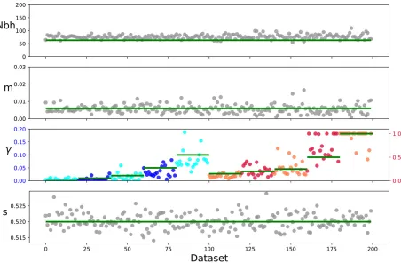
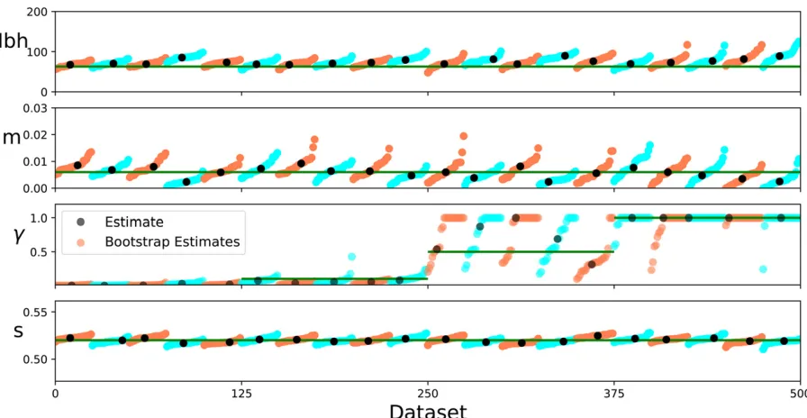
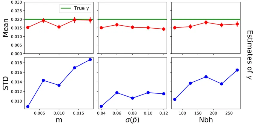
We investigated the overall capability of this method to estimate barrier strengths and the accuracy of empirical bootstrap uncertainty estimates. Our tests show that the in-ference scheme can reliably recover barrier strengths as well as demographic parameters (Figure 5 and Figure 7). Esti-mates of the neighborhood size are robust, but show a slight upward bias. These slight biases are likely due to the fact that a continuous model is used to fit to discrete simulations. Estimates of the long-distance migration rate m are more variable, but are not significantly biased. In all cases, the range of bootstrap estimates mostly overlaps with the true value to the expected degree. This result indicates that boot-strapping gives accurate uncertainty estimates (Figure 7).
The power to infer a barrier depends on several factors, including the particular sampling scheme, the number of sampled loci, various demographic parameters, as well as the strength of the barrier. We simulated several specific scenarios to explore overall patterns. Our results indicate that
estimates of the barrier strength g get more variable with increasingg(Figure 5, notice the two different scales). Weak barriers (g0:5) were sometimes inferred as no barrier at all, and vice versa. In contrast, strong barriers (g,0:1) were mostly also estimated as such. When varying demographic parameters, estimation uncertainty ofggrows with increas-ing long-distance migration rate mand neighborhood size (Figure 6). Changing the variance of the mean allele frequen-cies has comparatively little effect. In addition, we performed power simulations for varying numbers of sampled loci and sampled individuals. They indicate that at least a few dozen biallelic markers and several hundred samples are needed to robustly infer a strong barrier to geneflow (File S2).
Secondary contact:Barriers to geneflow sometimes coincide
with areas of secondary contact, for instance in secondary hybrid zones (Barton and Hewitt 1985). Allele frequencies might have diverged before this contact, and present day allele-frequency differences are not caused by the presence of a barrier. However, these clines resemble the effect of a barrier and might be mistakenly inferred as such. One salient way to deal with this problem is to remove markers that show a large-scale geographic structure of allele frequency. One can base inference on a subset of markers that have a similar mean allele frequency across the whole population range and only displayfluctuations on small geographic scales, which equilibrate quickly (Barton et al.2013). We tested this ap-proach on simulated data. When applying the inference scheme to a simulated scenario of secondary contact with divergent allele frequencies, it wrongly infers a barrier in case of nofiltering (File S2). However, when using the subset of loci that show no large-scale correlation with geography, the false positive signal decreases. Moreover, filtering out loci with a large-scale structure does not remove the signal in
case of a true barrier (File S2). However, if sampling is only done on small spatial scales, such filtering could become problematic as one might remove signal from localfl uctua-tions as well. Therefore, we advise to always check that the sampling area is bigger than the spatial scale of isolation-by-distance patterns before any markers are removed.
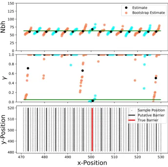
Unknown barrier locations:Our inference scheme assumes
that the location of the putative barrier is knowna priori. In practice, one might not always have this information or one perhaps wants to test the hypothesis of barriers in different locations. In this case, one can repeatedly apply the inference scheme and fit different potential barrier positions. When testing this approach on simulated data, the inference scheme only inferred a strong barrier near the true position (Figure 7 and Figure 8). The estimated uncertainties on the habitat edges are inflated. This effect is caused by limited power to infer barriers near sampling edges: one needs a sufficient number of samples on both sides of a barrier tofit the strength of a barrier.
Hybrid-zone analysis
We observed a clear isolation-by-distance pattern across the
Antirrhinumhybrid zone (Figure 9). On average, mean iden-tity by state for nearby plants is elevated by2% above the background level, and falls away with increasing pairwise
distance, most rapidly over the first 2000 m. Our inference scheme fits this pattern well, with an estimated neighbor-hood size of 188 (95% bootstrap confidence interval: 1202240;Figure 10).
Obviously, there are demographic complications that are not captured by our model, such as heterogeneities in plant distributions and density. The population is not distributed uniformly in two dimensions, as plants are often found in patches of suitable habitat (Figure 10). However, our analysis indicates that isolation-by-distance patterns are neither strongly influenced by the cardinal direction or relative plant positions, nor the geographic location within the hybrid zone (File S3). These observations imply that our model assump-tions are not grossly violated.
For putative barriers in the center of the hybrid zone, our inference scheme estimates no barrier (g.1). Bootstrap es-timates rarely fall belowg¼0:5;and all of them are above
g¼0:1: When testing for barriers toward theflank of the hybrid zone, estimates get more variable. Some estimates in bothflanks indicate an intermediate barrier to geneflow, but in each case some of the corresponding bootstrap esti-mates also take the value of no barrier (g.1). This signal likely reflects the lower power to infer barriers in these re-gions, as there is a higher sampling density in the center of the hybrid zone (58:7% of the samples originate from within 500 m of theflower-color transition). Only in one case, for the
leftmost tested barrier, the bootstrap estimates do not over-lap with the value of the null hypothesis (g¼1:0). This area also shows the strongest small-scale isolation-by-distance pattern (File S3), and the density of plants is very low in sampled patches (M. Melo, personal communication). Therefore, a potential explanation for this significant devi-ation from the null hypothesis of constant demography and no barrier to geneflow is an exceptionally low plant density in this area.
Given the overall goodfit of isolation by distance with our inference scheme (Figure 9), our results indicate that there is no strong genome-wide barrier to contemporary geneflow that coincides with the flower-color transition. As such a strong barrier would require many barrier loci spaced densely throughout the genome (Barton and Bengtsson 1986), this result comes as no surprise. At the moment, no other traits apart fromflower color are known to be divergent across the hybrid zone, despite much work to detect them (M. Melo, personal communication).
Previous results suggest the presence of a barrier to exchanging flower-color alleles (Whibley et al. 2006; Bradleyet al. 2017) and indicate that selection maintains differences in flower color (Ellis 2016). Therefore, we ap-plied our method to a subset of polymorphic markers in the genetic neighborhood of two genes,RoseaandEluta, known to affectflower-color variation in the hybrid zone. However, bootstrap estimates varied widely for all tested barrier loca-tions (results not shown), which indicates that there is not sufficient signal in the data. This lack of power is likely due to the low number of suitable SNP markers without steep allele-frequency clines near this region in our data set (,10). Simulations confirmed that for such a low number of markers there is not enough power to detect even strong barriers (File S2).
Discussion
To our knowledge, our scheme is thefirst method that infers the strength of the barrier based on an explicit spatial pop-ulation genetic model. There are several similarities with the inference method BEDASSLE (Bradburdet al.2013), which aims to disentangle the effects of geographic isolation by distance and differences in ecological variables. This scheme is not based on an explicit population genetic model, but ratherfits the decay of genetic similarity with distance to a heuristic formula. In light of possibly very complex demo-graphic structures, this approach is not necessarily worse thanfitting our spatial model. However, this approach does not take the increased covariances on the same side of a barrier into account, and does not make use of some valuable signal because of that. Moreover, it uses an MCMC approach that is based on a model of Gaussian randomfields, which is computationally too expensive to apply to hundreds or even thousands of individuals or demes. In contrast, our method is well suited to data sets of this magnitude.
Another widely used method to infer barriers to geneflow, Geneland, clusters individuals using their explicit geographic coordinates (Guillotet al.2005). Safneret al.(2011)
identi-fied it as one of the most potent methods to infer barriers to geneflow. Therefore, we tested its performance on some of the data sets which we have generated to test our scheme (File S4). As described previously (Guillot and Santos 2009; Safneret al.2011), Geneland’s ability to accurately infer bar-riers to geneflow decreases when isolation-by-distance pat-terns are present, as its underlying model assumptions of discrete populations with well-defined allele frequencies are violated. Indeed, it fails to detect a barrier to geneflow in our test data sets, which all exhibit such isolation-by-dis-tance patterns (File S4). In contrast, the method introduced here can give accurate estimates of the barrier strength in these scenarios. It is not confounded by isolation-by-distance patterns; in fact, it relies on the presence of this signal. Our method can therefore be seen as complementary to Geneland.
In contrast to BEDASSLE, Geneland, and most other exist-ing methods, which all heuristically describe the strength of the parameter; the inference scheme introduced herefits an explicit spatial population genetics model. It corresponds to Nagylaki’sg(Nagylaki 1978), whose inverse 1=gis equal to Barton’s barrier strength B (Barton and Bengtsson 1986). This correspondence makes the inferred barrier strength parameter ginterpretable directly in terms of population genetic theory. For instance, the parameterB=s2;which has a dimension of time, must be large to retard the spread of even a neutral allele (Barton and Bengtsson 1986).
Our method can reliably estimate the presence of strong barrier (g,0:1), but there is little power to distinguish be-tween a weak barrier and no barrier (Figure 5 and Figure 7). The reason for this is not a shortcoming of our inference scheme, but due to the fact that relatively weak barriers do not significantly affect the spread of ancestry (Figure 2).
Figure 9 Decay of pairwise homozygosity with geographic distance for hybrid zone data. All pairwise homozygosities for the filtered data set were binned according to pairwise distance. We also plot the best fit (Nbh¼188;m¼4:431024;s¼0:5247). Equation 10 can be used to
Therefore, it is infeasible to estimate the strength of weak barriers to gene flow, simply because they do not have a significant effect on allele frequency covariances. This effect was already observed by Bartonet al.(2013), who found that in two spatial dimensions the effect of a barrier starts to have appreciable effects on the spatial pattern of genetic marker alleles when barrier strengthB(which corresponds to 1=g) iss:
The exact power of the inference method depends on a range of factors. As a barrier mostly affects nearby allele-frequencyfluctuations, a high sampling density spread evenly on both sides of a putative barrier is ideal (Figure 8). Our results demonstrate that estimates of the barrier strength get more variable for increasing long-distance migration/muta-tion rate, or increasing neighborhood size (Figure 6). These patterns are not surprising, since the strength of isolation by distance, which constitutes the signal for our inference method, decreases whenmor Nbh grow. Our method is data hungry as it needs at least a few dozen SNP markers and at least hundreds of sampled individuals (File S2). This wealth of data is required since recent pairwise coalescence events, which constitute the signal for our inference scheme, are rare events in most realistic scenarios. As a rough rule of thumb,
our inference scheme can be applied in cases in which there is sufficient power to detect an overall isolation-by-distance pattern.
Any realistic scenario has its own set of parameters and specific sampling scheme. Our power simulations can only test a tiny fraction of possible combinations of these. They helped to elucidate general underlying patterns, but cannot cover all specific cases. Therefore, we recommend doing customized power simulations. Simulating the specific sampling scheme, the marker number together with likely demographic param-eters will help to determine whether the inference scheme has sufficient power to detect putative barriers for the specific scenario of interest.
Outlook
The inference scheme introduced here fits a linear barrier, the most straightforward model for a barrier in two dimen-sions. We used an analytical formula (Equation 5) to model the spread of ancestry, which in turn allows one to reduce calculations for pairwise F to a single numerical integral (Equation 7). However, barriers might be geographically more complex in practice. There could also be multiple bar-riers in different locations which would be partly indicated by
our method, but also invalidate its underlying model of a single barrier. Such more-complicated scenarios will most likely not allow for simple formulas, and calculations for the chances of recent coancestry become much more chal-lenging. One could trace the geographic ancestry distribution back with discretized simulations, and use them tofirst cal-culate the expected distributions of recent pairwise coales-cence (Equation 6) and consequently identity-by-descent patterns (Equation 7). This salient extension to our model poses a numerical challenge, but it seems to be within reach of present day computational power.
Our methodfits allele frequencies that can be confounded by deeper ancestral patterns. Byfiltering loci that show large-scale geographic variation, one can in principle remove some of this ancestral genetic structure, but one might accidentally remove true signal as well by doing so. This problem can be a severely confounding factor when applying the inference method to scenarios where ancestral structure is present, for instance in zones of putative secondary contact.
One promising way to overcome this problem would be to base inference on identity-by-descent blocks, the direct ge-netic traces of recent coancestry (Browning and Browning 2012). As blocks of ancestral genetic material are split up at a constant rate by recombination, the probability of sharing a block of lengthldecays exponentially back in time (Ralph and Coop 2013). For example, blocks .5 cM are therefore very unlikely to originate from coancestry older than 100 gen-erations, even under relatively extreme demographic scenar-ios. Moreover, the length of the blocks contains information about the time of coalescence. Identifying such blocks is a nontrivial task, particularly when only unphased genotype data are available (Browning and Browning 2012), as it requires dense genotype data and linkage information. But in cases where identity-by-descent blocks can be robustly called—as is already possible for humans and some model organisms—an inference scheme based on this signal holds great potential. Our method to model the spread of ancestry can be combined with formulas for block sharing (Ralph and Coop 2013; Ringbaueret al.2017) to calculate the expected number of shared identify-by-descent blocks in presence of a barrier. These results could be used to fit observed block-sharing data.
In summary, our method is only afirst step to robustly infer barriers to gene flow from genotype data. The techniques outlined here can be expanded in various directions to better deal with the complexities of real data and to make full use of the opportunities within the era of population genomics. We hope that this will ultimately lead to a better understanding of barriers to geneflow within many natural populations.
Acknowledgments
We thank Himani Sachdeva and Raphaël Forien for several useful discussions and for comments on previous drafts of this article. We thank Maria Melo for many discussions about the Antirrhinum system, as well as members of the
Barton and Coen laboratory and many volunteers for orga-nizing and carrying out thefield work that gave rise to the data set analyzed here. We thank Jon Wilkins and an anon-ymous reviewer for their very helpful suggestions on how to improve the manuscript.
Literature Cited
Aguillon, S. M., J. W. Fitzpatrick, R. Bowman, S. J. Schoech, A. G.
Clarket al., 2017 Deconstructing isolation-by-distance: the
ge-nomic consequences of limited dispersal. PLoS Genet. 13: e1006911.
Barton, N. H., 1979 Geneflow past a cline. Heredity 43: 333–339.
Barton, N. H., 2008 The effect of a barrier to geneflow on
pat-terns of geographic variation. Genet. Res. 90: 139–149.
Barton, N. H., and G. M. Hewitt, 1985 Analysis of hybrid zones.
Annu. Rev. Ecol. Syst. 16: 113–148.
Barton, N. H., and B. O. Bengtsson, 1986 The barrier to genetic
exchange between hybridising populations. Heredity 57: 357–376.
Barton, N. H., F. Depaulis, and A. M. Etheridge, 2002 Neutral
evolution in spatially continuous populations. Theor. Popul.
Biol. 61: 31–48.
Barton, N. H., A. M. Etheridge, J. Kelleher, and A. Véber, 2013 Inference
in two dimensions: allele frequenciesvs.lengths of shared
se-quence blocks. Theor. Popul. Biol. 87: 105–119.
Bradburd, G. S., P. L. Ralph, and G. M. Coop, 2013 Disentangling
the effects of geographic and ecological isolation on genetic
differentiation. Evolution 67: 3258–3273.
Bradley, D., P. Xu, I.-I. Mohorianu, A. Whibley, D. Field et al.,
2017 Evolution offlower color pattern through selection on
regulatory small RNAs. Science 358: 925–928.
Browning, S. R., and B. L. Browning, 2012 Identity by descent
between distant relatives: detection and applications. Annu.
Rev. Genet. 46: 617–633.
Cercueil, A., O. François, and S. Manel, 2007 The genetical
band-width mapping: a spatial and graphical representation of pop-ulation genetic structure based on the wombling method. Theor.
Popul. Biol. 71: 332–341.
Dupanloup, I., S. Schneider, and L. Excoffier, 2002 A simulated
annealing approach to define the genetic structure of
popula-tions. Mol. Ecol. 11: 2571–2581.
Ellis, T. J., 2016 The role of pollinator-mediated selection in the
maintenance of aflower color polymorphism in an Antirrhinum
majus hybrid zone. Ph.D. Thesis, IST Austria, Klosterneuburg, Austria.
Falush, D., M. Stephens, and J. K. Pritchard, 2003 Inference of
population structure using multilocus genotype data: linked loci
and correlated allele frequencies. Genetics 164: 1567–1587.
Fisher, R. A., 1937 The wave of advance of advantageous genes.
Ann. Eugen. 7: 355–369.
Forien, R., 2017 Geneflow across geographical barriers - scaling
limits of random walks with obstacles. arXiv preprint arXiv: 1711.02589.
Grebenkov, D. S., D. Van Nguyen, and J.-R. Li, 2014 Exploring
diffusion across permeable barriers at high gradients. I. Narrow
pulse approximation. J. Magn. Reson. 248: 153–163.
Guillot, G., and F. Santos, 2009 A computer program to simulate
multilocus genotype data with spatially autocorrelated allele
frequencies. Mol. Ecol. Resour. 9: 1112–1120.
Guillot, G., A. Estoup, F. Mortier, and J. F. Cosson, 2005 A spatial
statistical model for landscape genetics. Genetics 170: 1261–
1280.
Guillot, G., R. Leblois, A. Coulon, and A. C. Frantz, 2009 Statistical
Hardy, O. J., and X. Vekemans, 1999 Isolation by distance in a continuous population: reconciliation between spatial autocor-relation analysis and population genetics models. Heredity 83:
145–154.
Laporte, V., and B. Charlesworth, 2002 Effective population size
and population subdivision in demographically structured
pop-ulations. Genetics 162: 501–519.
Malécot, G., 1948 Les mathématiques de l’hérédité. Masson et Cie,
Paris.
Manni, F., E. Guerard, and E. Heyer, 2004 Geographic patterns of
(genetic, morphologic, linguistic) variation: how barriers can be
detected by using monmonier’s algorithm. Hum. Biol. 76: 173–
190.
Meirmans, P. G., 2012 The trouble with isolation by distance.
Mol. Ecol. 21: 2839–2846.
Nagylaki, T., 1978 A diffusion model for geographically
struc-tured populations. J. Math. Biol. 6: 375–382.
Nagylaki, T., 1988 The influence of spatial inhomogeneities on
neutral models of geographical variation: I. Formulation. Theor.
Popul. Biol. 33: 291–310.
Nagylaki, T., 1998 The expected number of heterozygous sites in
a subdivided population. Genetics 149: 1599–1604.
Ralph, P., and G. Coop, 2013 The geography of recent genetic
ancestry across Europe. PLoS Biol. 11: e1001555.
Ringbauer, H., G. Coop, and N. H. Barton, 2017 Inferring recent
demography from isolation by distance of long shared sequence
blocks. Genetics 205: 1335–1351.
Rousset, F., 1997 Genetic differentiation and estimation of gene
flow from f-statistics under isolation by distance. Genetics 145:
1219–1228.
Rousset, F., 2002 Inbreeding and relatedness coefficients: what
do they measure? Heredity 88: 371–380.
Safner, T., M. P. Miller, B. H. McRae, M.-J. Fortin, and S. Manel,
2011 Comparison of Bayesian clustering and edge detection
methods for inferring boundaries in landscape genetics. Int.
J. Mol. Sci. 12: 865–889.
Slatkin, M., 1993 Isolation by distance in equilibrium and
non-equilibrium populations. Evolution 47: 264–279.
Whibley, A. C., N. B. Langlade, C. Andalo, A. I. Hanna, A. Bangham
et al., 2006 Evolutionary paths underlyingflower color
varia-tion in antirrhinum. Science 313: 963–966.
Wilkins, J. F., 2004 A separation-of-timescales approach to the
co-alescent in a continuous population. Genetics 168: 2227–2244.
Womble, W. H., 1951 Differential systematics. Science 114: 315–
322.
Wright, S., 1943 Isolation by distance. Genetics 28: 114.
Appendix
Here we give the full formula wefit and describe the rescaling of a set of independent effective parameters. Letx1;x2denote the x-coordinate of the samples andDxð¼x12x2ÞandDytheir separation along each axis. For the identity by state on different sides of the barrier, plugging into Equation 7 gives for pairwiseF:
Z N
0
1 2De
exp 4k
s2ðDxþ4ktÞ !
2k s2erfc
Dxþ8kt ffiffiffiffiffiffiffiffiffiffi 4s2t p
|fflfflfflfflfflfflfflfflfflfflfflfflfflfflfflfflfflfflfflfflfflfflfflfflfflfflfflfflfflfflfflfflfflfflfflfflfflfflffl{zfflfflfflfflfflfflfflfflfflfflfflfflfflfflfflfflfflfflfflfflfflfflfflfflfflfflfflfflfflfflfflfflfflfflfflfflfflfflffl} Movement x2axis
1 ffiffiffiffiffiffiffiffiffiffiffiffiffi 4ps2t
p exp 2ðDyÞ
2
4s2t !
|fflfflfflfflfflfflfflfflfflfflfflfflfflfflfflfflfflfflfflfflffl{zfflfflfflfflfflfflfflfflfflfflfflfflfflfflfflfflfflfflfflfflffl} Movement y2axis
expð22mtÞ dt |fflfflfflfflfflfflfflfflfflfflffl{zfflfflfflfflfflfflfflfflfflfflffl}
mutation :
We now rescale time such thatt9¼s2t:The integral (dt9¼s2dt) transforms to: Z N
0 ffiffiffiffi p
p ffiffiffiffi t9
p 2k
4pDes4exp 4k s2
Dxþ4k s2t
!
erfc Dxþ4
2k s2t 2pffiffiffiffit9
!
exp 2ðDyÞ
2
4t9 !
exp
22m
s2t
dt9:
Defining Nbh:¼4pDes2;g:¼2k=s2;andm¼2m=s2gives the full formula used for inference:
Z N
0
1 Nbh
ffiffiffiffi p t9 r
expð2gðDxþ2gtÞÞgerfc
Dxþ4gt
2pffiffiffiffit9
exp 2ðDyÞ
2
4t9 !
expð2mtÞdt9:
The formula for the same sides of the barrier is rescaled analogously. The additional term in the integrand becomes:
1 Nbh
1 2t
(
exp 2ðx12x2Þ
2
4t9 !
þexp ðx1þx2Þ
2
4t9 !)
exp 2ðDyÞ
2
4t9 !