ABSTRACT
KIM, JANET S. Flexible Regression Models for Functional Responses. (Under the direction of Ana-Maria Staicu.)
Regression models where both the response and the covariate are curves have become
in-creasingly common in many scientific fields including medicine, finance, and agriculture, to
name a few. These problems are often called function-on-function regression, and their primary
goal is to identify associations between the response and predictor functional variables. In the
first part of the thesis, we introduce a flexible regression model to study the association between
a functional response and a functional covariate that are observed on the same domain. Our
modeling describes the relationship between the mean current response and the covariate by a
smooth unknown bi-variate function that depends on both the current value of the covariate and
the time point itself. We develop estimation methodology that accommodates realistic scenarios
where the covariates are sampled with or without error on a sparse and/or irregular design, and
prediction that accounts for unknown model correlation structure. In this framework we also
discuss the problem of testing the null hypothesis that the covariate has no association with
the response. The proposed methods are evaluated numerically through simulations and two
real data applications.
In the second part of the thesis, we consider non-linear regression models for functional
responses and functional predictors observed on possible different domains. We introduce
flex-ible models where the mean response at a particular time point depends on the time point
itself as well as the entire covariate trajectory. In this framework, we develop computationally
efficient estimation methodology and discuss prediction of a new response trajectory. We
pro-pose an inference procedure that accounts for total variability in the predicted response curves,
and construct point-wise prediction intervals. The proposed estimation/inferential procedure
accommodates realistic scenarios such as correlated error structure as well as sparse and/or
two real data applications.
In the third part of the thesis, we propose a method for testing linearity in
function-on-function regression models for function-on-functional responses and predictors that are observed on possible
different domains. Specifically, we discuss the problem of testing the null hypothesis that the
covariate has a linear association with the response against a complex non-linear dependence
structure. The alternative hypothesis assumes a flexible dependence structure and models their
relationship through smooth tri-variate function that depends on the current time point as
well as the entire covariate trajectory, where estimation of this type of models are discussed in
the previous chapter. The null hypothesis is tested by representing this general additive class
of models using a linear mixed effects model representation and then by testing the variance
component with a nuisance variance component under the null hypothesis. Its size and power
properties are assessed through simulations under various realistic scenarios and two real data
© Copyright 2016 by Janet S. Kim
Flexible Regression Models for Functional Responses
by Janet S. Kim
A dissertation submitted to the Graduate Faculty of North Carolina State University
in partial fulfillment of the requirements for the Degree of
Doctor of Philosophy
Statistics
Raleigh, North Carolina
2016
APPROVED BY:
Arnab Maity David Dickey
Yichao Wu Ana-Maria Staicu
DEDICATION
BIOGRAPHY
Janet S. Kim was born in Cleveland, Ohio on November 4, 1984 and grew up in Pohang,
Republic of Korea. She received a Bachelor of Science with majors in Mathematics and Statistics
in August of 2008 from Ewha Womans University, Seoul, Republic of Korea. She earned a Master
of Science in Mathematics in August of 2010 from Ewha Womans University. She moved to
Raleigh, North Carolina in August of 2010 to pursue graduate studies in Statistics at North
Carolina State University. She earned a Master of Statistics degree in May of 2012 and her PhD
ACKNOWLEDGEMENTS
I wish to express my deepest gratitude to my Advisor, Ana-Maria Staicu, for her support and
guidance throughout my graduate career. This research would not have been possible without
her dedication and endless encouragement. In particular, I appreciate her special commitement
to advising me whenever I encountered difficulties in my personal life as well as in my
profes-sional development. I would like to sincerely thank Arnab Maity for collaborating and providing
invaluable input necessary to complete the research contained in this dissertation. I would like
to thank my committee members, Yichao Wu and David Dickey, for providing valuable insights
into this research. I also thank Siamak Khorram for serving as the graduate school
represen-tative on my committee. To all of the faculty and the staff in Statistics department at North
Carolina State University (NCSU), I extend my appreciation.
To my family: I thank you for your love, encouragement, patience, and support throughout
this process. Most importantly, I have the deepest gratitude for mom. She has continually given
guidance and support to find my own life and to overcome difficult situations. I am grateful to
my dad for teaching me to do all my best at every moment. I thank my sister, Christine, for
helping family members in family medical emergency situations during my PhD studies.
Finally, to my husband, Taek: Your support, humor, and exceeding love brought this success.
TABLE OF CONTENTS
List of Tables . . . .viii
List of Figures . . . x
Chapter 1 Introduction . . . 1
1.1 Modeling the Functional Data . . . 1
1.2 Smoothing . . . 4
1.2.1 Smoothing Based on Known Basis Functions Expansions . . . 4
1.2.2 Smoothing through Roughness Penalties . . . 6
1.2.3 Data-Driven Basis Expansions . . . 7
1.3 Regression Models for Functional Responses and Functional Covariates . . . 9
Chapter 2 General Functional Concurrent Model . . . 12
2.1 Introduction . . . 12
2.2 General Functional Concurrent Model . . . 14
2.2.1 Modeling Framework . . . 14
2.2.2 Estimation . . . 16
2.2.3 Variance Estimation . . . 17
2.2.4 Prediction . . . 18
2.3 Hypothesis Testing . . . 20
2.4 Transformation of Functional Covariate . . . 22
2.5 Extensions . . . 23
2.5.1 Data-Processing for Irregular and Sparse Design . . . 23
2.5.2 Model Estimation for Irregular and Sparse Design . . . 24
2.5.3 Model Estimation for Multiple Predictors . . . 25
2.6 Numerical Study . . . 28
2.6.1 Details of Simulation Setup . . . 28
2.6.2 Simulation Results . . . 31
2.6.3 Applications . . . 37
Chapter 3 General Additive Function-on-Function Regression . . . 43
3.1 Introduction . . . 43
3.2 Methodology . . . 45
3.2.1 Statistical Framework and Modeling . . . 45
3.2.2 Estimation and Prediction . . . 47
3.3 Out-of-Sample Prediction and Inference . . . 49
3.3.1 Estimation of Error Covariance . . . 50
3.3.2 Out-of-Sample Prediction Inference . . . 51
3.4 Implementation and Extensions . . . 53
3.5 Simulation Study . . . 55
3.5.1 Details of Simulation Setup . . . 55
3.5.3 Simulation Results . . . 59
3.6 Applications . . . 62
3.6.1 Capital Bike Share Data . . . 62
3.6.2 Yield Curves Data . . . 66
Chapter 4 Testing for Linearity in General Additive Function-on-Function Regression . . . 69
4.1 Introduction . . . 69
4.2 Restricted Likelihood Ratio Tests in Function-on-Function Regression . . . 72
4.2.1 Testing Procedure . . . 72
4.2.2 Review of Restricted Likelihood Ratio Tests in Scalar-on-Function Re-gression . . . 75
4.3 Data Preprocessing . . . 76
4.3.1 Transformation of Covariate . . . 76
4.3.2 Data Pre-processing for Sparse Sampling Design . . . 76
4.4 Simulation Study . . . 77
4.4.1 Simulation Setup . . . 77
4.4.2 Competitive Method . . . 79
4.4.3 Simulation Results . . . 80
4.5 Applications . . . 86
4.5.1 Capital Bike Share Study . . . 86
4.5.2 US Yield Curves Study . . . 87
Chapter 5 Conclusion . . . 89
REFERENCES . . . 92
APPENDICES . . . 97
Appendix A Additional Details for Chapter 2 . . . 98
A.1 Additional Simulation Results . . . 98
A.1.1 Further Investigation of Prediction Error . . . 98
A.1.2 Further Investigation of Different Covariance Estimation Methods . 102 A.1.3 Further Investigation of Computation Time . . . 102
A.2 Further Investigation of Gait Data Example . . . 104
A.3 Implementation Details . . . 109
Appendix B Additional Details for Chapter 3 . . . 111
B.1 Additional Simulation Results . . . 111
B.1.1 Additional Simulations for Irregular and Sparse Design . . . 111
B.1.2 Sensitivity Analysis . . . 112
B.2 Further Investigation of Real Data Example . . . 112
B.2.1 Histogram of Standardized Average Humidity . . . 112
B.2.2 Validation of L2-Norm Based Test . . . 113
Appendix C Additional Details for Chapter 4 . . . 116
LIST OF TABLES
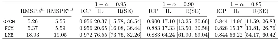
Table 2.1 Summary of RMSPEin, RMSPEout, ICP, IL, and R(SE) based on 1000 simulated data sets. The models fitted by our method and the linear FCM are indicated byGFCM and FCM, respectively. . . 32 Table 2.2 Rejection probabilities (×100) atα= 5% and 10% significance levels. The
values in the parenthesis are the estimated standard errors (×100) of the rejection probabilities. . . 35 Table 2.3 Results from Gait data example. Displayed are the summaries of RMSPEin,
RMSPEout, ICP, IL, and R(SE). The models fitted by our method and the
linear FCM are indicated byGFCM and FCM, respectively. . . 38 Table 2.4 Results from the calcium absorption data example. Displayed are the
sum-maries of RMSPEin, RMSPEout, ICP, IL, and R(SE). The models fitted by our method and the linear FCM are indicated byGFCMandFCM, respectively. 41
Table 3.1 Summary of (1) RMSPEin and (2) RMSPEout based on 1000 simulated data sets. Results correspond to fitting the method of GAFFR and FLM. . 59 Table 3.2 Comparisons withFAMandSFFin terms of (1) RMSPEinand (2) RMSPEout,
and (3) computation time (in seconds) averaged over 1000 simulations. Re-sults correspond to the cases withn= 50. . . 60 Table 3.3 Summary of average coverage probability (ACP) for the new response
Y0,i0(t)|X0,i0(·) at nominal significance levels 1−α =0.85, 0.90, and 0.95.
The results are based on 1000 simulated data sets with 100 bootstrap replications per data. . . 61 Table 3.4 Summary of (1) RMSPEin and (2) RMSPEout in bike share data analysis. 64
Table 4.1 Type I error rates (×100) for dense sampling design (mW = 51, mY = 81 for alli) based on 2000 Monte Carlo simulations. The values in the paren-thesis are the estimated standard errors (×100) of the rejection probabil-ities. Results corresponding to the proposed test and the bootstrap-based algorithm are indicated by pRLRTand bootstrap, respectively. . . 82 Table 4.2 Type I error rates (×100) for sparse sampling design (mW,i ∼ {37, . . . ,42},
mY,i ∼ {59, . . . ,64}) based on 2000 Monte Carlo simulations. The values in the parenthesis are the estimated standard errors (×100) of the re-jection probabilities. Results corresponding to the proposed test and the bootstrap-based algorithm are indicated bypRLRTandbootstrap, respec-tively. . . 83
Table A.1 Summary of RMSPEin, RMSPEout, ICP, IL, and R(SE) for a moderately sparse design. The models fitted by our method and the linear FCM are indicated by GFCMand FCM, respectively. . . 99 Table A.2 Summary of RMSPEinand standard deviations (in parentheses) obtained
Table A.3 Summary of RMSPEinand standard deviations (in parentheses) obtained by fitting the GFCM based on 1000 simulations. The simulation settings correspond to the case whereEi =E3i. Reduced variance is used to generate the covariate trajectories. . . 101 Table A.4 Summary of ICP, IL, and R(SE) for sample size 100 and Ei = E3i based
on 1000 simulations. . . 103 Table A.5 Summary of (1) RMSPEin, (2) RMSPEout, and (3) average computation
time in seconds obtained by fitting the GFCM based on 1000 simulations. The left (right) table is obtained by using gam (bam) function of mgcv R package. . . 105 Table A.6 Summary of RMSPEin, RMSPEout, ICP, IL, and R(SE) obtained from
the simulation studies of the gait data example. The models fitted by our method and the linear FCM are indicated by GFCMand FCM, respectively. . 108
Table B.1 Summary of (1) RMSPEin and (2) RMSPEout based on 1000 simulated data sets. . . 112 Table B.2 Summary of (1) RMSPEin and (2) RMSPEout based on 1000 simulated
data sets. Results are obtained by applying the GAFFR model. . . 113 Table B.3 Summary of ACP for the new responseY0(t)|X0(·), i.e., ACPp, at nominal
significance levels 1−α=0.85, 0.90, and 0.95. Results are based on 1000 simulated data sets with 100 bootstrap replications per data. . . 113 Table B.4 Summary of estimated rejection probabilities (×100). The values in the
parenthesis are the estimated standard errors (×100) of the rejection prob-abilities. . . 115
Table C.1 Type I error rates (×100) for sparse sampling design (mW,i ∼ {27, . . . ,32},
LIST OF FIGURES
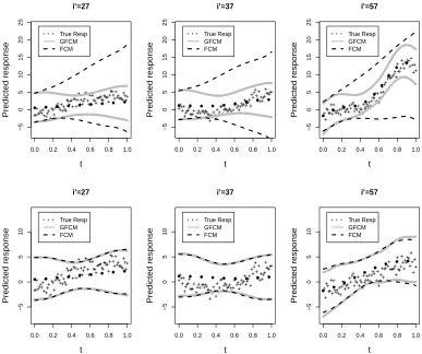
Figure 2.1 Comparison of 95% prediction bands constructed for three subject-level trajectories in the test data. The case corresponds to a dense design with 100 subjects and E3i error structure. “+” are the response Y0,i0(·) in the
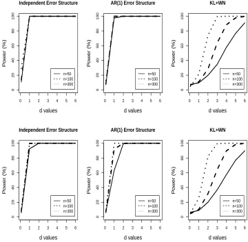
test data, and dotted (“•”) lines are the true response without measure-ment errors. Solid and dashed lines are the prediction bands obtained by fitting the GFCM and the linear FCM, respectively. The top (bottom) panel corresponds to the case when the true function F is non-linear (linear). . . 34 Figure 2.2 Powers (×100) of the tests at significance levelα= 5%. The top (bottom)
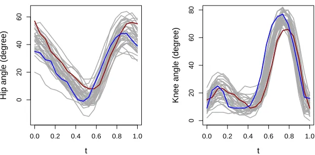
panel displays the result from the densely (sparsely) sampled. The error process in the left, middle and right panels is assumed to be E1i,E2i and E3i, respectively. . . 36 Figure 2.3 Longitudinal measurements of the hip angle (left) and the knee angle
(right) obtained from 39 children while they go through a single gait cycle. 37 Figure 2.4 Results from the gait data analysis. The top panel displays 95% prediction
bands obtained by fitting the GFCM (grey solid lines) and the linear FCM (dashed lines) for three subject-level trajectories in the test data. “•” represent the knee angles in the test data. The bottom panel shows the heat map of Yb0,i0(t) obtained from the test data set of the gait data
example. . . 39 Figure 2.5 Longitudinal measurements of calcium intake (left) and calcium
absorp-tion (right) obtained from 188 patients. . . 40 Figure 2.6 Results from the calcium absorption data analysis. Displayed is 95%
pre-diction bands obtained by fitting the GFCM (grey solid lines) and the linear FCM (dashed lines) for three subject-level trajectories in the test data. “•” indicate the calcium absorption measured. Thin solid lines are the smoothed curve of the calcium absorption. . . 42
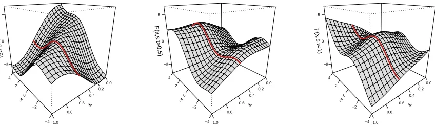
Figure 3.1 True surface of F3(x, s,0.05) (left), F3(x, s,0.5) (middle), and F3(x, s,1)
(right). The red solid line represents the curve obtained by fixing sas 0.6. 55 Figure 3.2 The number of casual bike users (left panel) and hourly temperatures
(right panel) collected every Saturday. The measurements taken in three different days on January, April, and July in 2011 are indicated by solid, dashed, and dotted lines, respectively. . . 63 Figure 3.3 Changes in the US yield curves (left panel) and in the European yield
curves (right panel) during the period from January 2, 2006 to December 30, 2011. The measurements taken in three different days are indicated by red, blue, and green lines. . . 67
Figure 4.1 True surface of F2(x, s,0.55) corresponding to the model under the null
Figure 4.2 Power (×100) of the tests at significance level α = 5% based on 1000 Monte Carlo simulations. Results are for the proposed RLRTs in the case F(x, s, t) =F2(x, s, t) and Ei =E3i. The left and right panel correspond to the dense and sparse sampling design, respectively. . . 84 Figure 4.3 Power (×100) of the tests at significance level α = 5% based on 1000
Monte Carlo simulations. The left most two panels correspond to the case where E1i and E2i. The right most two panels correspond to E3i and E4i, respectively. Results for F(x, s, t) =F1(x, s, t) and F(x, s, t) =F2(x, s, t)
are displayed in the top and bottom row, respectively. . . 85
Figure A.1 Displayed plots are curves for sample size 100 simulated based on the gait data. The smoothed version of covariate functions Xbisim are presented in
the left. The middle and the rightmost panel present response curvesYi(t) generated based on FL,gait(x, t) and FNL,gait(x, t), respectively. The last two subjects are highlighted in different colors. . . 106
Chapter 1
Introduction
1.1
Modeling the Functional Data
Functional data analysis (FDA) has become increasingly important due to the advent of
compu-tations and technology that allow measurements to be taken on very fine grids; for a
comprehen-sive review of FDA, refer to the monograph by Ramsay and Silverman (2005); Ferraty and Vieu
(2006); Ramsay, Hooker and Graves (2009), among many others. An example of functional data
is chemometric data (Ferraty and Vieu, 2003; Ferraty and Vieu, 2006). The chemometric data
consists of a 100 channel spectrum of light absorbances obtained from 240 samples of finely
chopped meat. For each sample, the absorbances are recorded on the Tecator Infratec food and
feed analyzer operating in the 100 different wavelengths between 850nm and 1050nm. As the
light absorption occurs at the wavelength sequentially, we can consider the absorbances from
each sample as a function of wavelength.
Although a function is defined over an infinite-dimensional space, in practice we observe
only a finite number of realization of the underlying process. In FDA, the observed data can be
with noise. This feature can be expressed by the model
Yij =Xi(tij) +ij, (1.1)
whereXi(tij) are the smooth latent curve fromith subject, andij are the errors with zero-mean
and unknown covariance. Specifically, it is assumed thatXi(t) are the square-integrable random
process with RT
XE{Xi(t)}
2dt < ∞. The number of observations, m
i, does not necessarily be
the same for each subject. When the data are observed on a fine and equally spaced grid, i.e.,
mi =m for all i, this setting is commonly referred to as dense design. The chemometric data correspond to the densely observed functional data. When the number of observations mi is
small, we call this setting sparse design. In the case of sparsely observed data, it is typically
assumed that the pooled time points across the subjects,S
i,jtij, are dense inTX.
Many theoretical and methodological developments have been undertaken in the FDA.
Major topics of interest are (i) to study important sources of variation in the curves and
(ii) to predict subject specific trajectories based on the observed data. A key research
di-rection is focused on studying the variability of curves. Functional principal component
anal-ysis (FPCA) is the methodology developed to deal with this type of problems; it determines
main directions of variability within the curves. FPCA is first employed by Rao (1958) and
developed for both dense (see e.g., Rice and Silverman, 1991; Hall and Hosseini-Nasab, 2006;
Cardot, 2007; Zhang and Chen, 2007) and sparse design (see e.g., Staniswalis and Lee, 1998;
James, Hastie and Sugar, 2000; Yao et al., 2005a). FPCA is coined differently, depending on
whether the sampling design is dense or fixed. If the design is dense, the common approach is
to smooth each individual curve to remove the noise and then to apply PCA to the smoothed
curves; Section 1.2 discusses several ways to smooth the curves. When the design is sparse,
the FPCA requires pooling the data together; this approach is also detailed in Section 1.2.3.
The standard FPCA methods facilitate reconstruction of full trajectories based on few
Various extensions and techniques have been studied up to date. Relevant research includes
Ramsay and Dalzell (1991) and Ramsay and Silverman (2005) for smoothing based on FPCA,
and Di et al. (2009) for multilevel FPCA, among many others. For a complete review of FPCA,
see Shang (2014).
Another main research direction is developing functional regression models, where one or
both of response and covariates have functional characteristics in the sense described above.
Scalar-on-function regression is a relevant area that has been developed to quantify a
rela-tionship between a scalar response and functional covariate/s. For example, functional
lin-ear model (see e.g., James, 2002; James and Silverman, 2005; M¨uller and Stadtm¨uller, 2005;
James, Wang and Zhu, 2009; Goldsmith et al., 2011) assumes that the effect of functional
co-variate is linear and predicts the scalar responses using the entire coco-variate trajectory through a
weighted integral. Sometimes, trends may not necessarily be captured linearly, and extensions of
the functional linear model to non-linear case are addressed in McLean et al. (2014).
Function-on-function regression framework also has been studied through various association models such
as functional concurrent model, functional historical linear model, and functional linear model
(for functional responses). The functional concurrent models (Ramsay and Silverman, 2005)
assume that the response profile at the current time point is only affected by the covariate
profile at the same time point. However, this type of models does not allow the past or future
observations of the covariate to affect the current response. Those cases are considered by the
functional historical models (see e.g., Malfait and Ramsay, 2003) and functional linear
mod-els (see e.g., Ramsay and Dalzell, 1991; Ramsay and Silverman, 2005; Yao, M¨uller and Wang,
2005b). The functional historical models predict the current response using the past
observa-tions of the covariate, whereas the functional linear models relates the current response using
the entire trajectory of the predictor.
In this thesis, we continue the study of regression models for function-on-function regression
to describe more general relationships between the response and the covariate. For the rest of
basis functions expansions with or without penalty and data-driven basis expansions in
Sec-tion 1.2. We discuss funcSec-tion-on-funcSec-tion regression in more detail with potential applicaSec-tions
in Section 1.3.
1.2
Smoothing
In FDA, smoothing the functional data is an essential procedure due to the representation
in (1.1). There are two important reasons for smoothing the data. One reason is to remove
the measurement errorsij from the observed data and recover the smooth underlying process
Xi(t). The other reason is to predictXi(t) at any values oftwhen only one or few observations
are available for each curve.
Smoothing can be achieved by using basis functions expansions, and the number of basis
functions used to represent the curve affects to the amount of smoothness. Several different types
of basis functions have been used in the literature. One of which is a known set of basis functions
such as splines, wavelets, and Fourier basis. When using the pre-specified set of basis functions,
one can further incorporate roughness penalty to further impose smoothness on the result.
The other choice is driven basis such as eigenbasis of a covariance function. The
data-driven basis is unknown and can be estimated from the observed data using FPCA techniques.
In the next subsequent sections, we introduce smoothing based on the known basis functions
expansions (Section 1.2.1), smoothing in conjunction with a roughness penalty (Section 1.2.2),
and the data-driven basis expansions (Section 1.2.3).
1.2.1 Smoothing Based on Known Basis Functions Expansions
The smooth latent process Xi(t) in (1.1) can be represented as a linear combination of known
basis functions. For illustration, we use B-spline basis functions of order 4 (cubic B-splines). Let
{bk(t) :k≥1} be a set of B-spline basis functions, and denote byK the number of basis
estimat-ing the basis coefficients is minimizestimat-ing the sum of squares criterionP
i=1||Yi(·)−PkK=1bk(·)βk||2 with respect toβk, where|| · ||2 corresponds to the commonL2-norm induced by the inner prod-uct< f, g >=Rf g.
The choice of basis functions has a little effect on the estimates Xbi(t). The
usual convention is to select based on the characteristics of the data. Fourier basis
{1,sin(2πt),cos(2πt),sin(4πt),cos(4πt), . . .}is often chosen when the data has periodic nature, and it is commonly used in signal processing. When the data has non-periodic trends, spline
basis functions such as B-splines and truncated power functions can be used. When there are
spikes in the curve, one would prefer wavelet bases. Since our study uses B-splines for the
representation of the models, we provide further details on the B-splines.
B-splines are developed by de Boor (1978) and have many attractive properties. B-splines
are constructed by polynomial pieces which connect smoothly at the joints and are useful to
represent a smooth curve. For example, cubic B-splines consist of four cubic polynomial pieces,
and their first and second derivatives are continuous at the joined points. We call the joined
pointsknots. Selecting the location of knots might be a challenging issue. When the resolution
of the curve is dense, we use equally-spaced knots. When the resolution of the curve is low, we
place more knots over regions where the function has high curvature. B-splines have compact
support and are locally non-zero. Due to this property, computing the expansion of B-splines is
relatively fast compared to the other basis expansions. For a comprehensive review of B-splines,
we refer the reader to Eilers and Marx (1996); Ruppert et al. (2003); Marx and Eilers (2005);
Ramsay and Silverman (2005); Wood (2006a).
The amount of smoothing can be controlled by selecting an optimal number of basis
func-tions. A large number of basis functions can accommodate the complexity of function, but the
estimated curve can be wiggly. A small number of basis functions can lead to overly smooth fit,
1.2.2 Smoothing through Roughness Penalties
We use penalized basis functions expansions (see e.g., Wahba, 1990; Ruppert et al., 2003; Wood,
2006a; Li and Ruppert, 2008) to balance the trade-off between goodness of fit as well as
smooth-ness of fit. The idea behind this approach is that we use a large number of basis functions to
fully capture the variability of the function, and impose a penalty to control the smoothness of
the resulting fit. In this approach, the penalty is often referred to as roughness penalty.
To illustrate the idea, consider model (1.1), and let Yi = [Yi1, . . . , Yimi]
T. An estimate of
the function Xi(t) can be obtained by minimizing the penalized criterion Pi=1||Yi−Xi(·)||2+
λPen(X), where the first term is the sum of squares criterion, and Pen(X) is the penalty that
measures variability of the functionXi(·). The parameterλis known as a smoothness parameter that controls the amount of penalization. The amount of penalization is associated with the
magnitude of the derivative of the function, X(r)(t), where r is the order of the derivative.
A common choice is the second derivative X00(t), and the size of curvature can be measured
through the integrated squared second derivativeR TX{X
00(t)}2dt. Then, the penalized criterion
to be minimized is given byP
i=1||Yi−Xi(·)||2+λ R
TX{X
00(t)}2dt.
If we represent the function Xi(t) using a basis functions expansion, the penalty Pen(X)
can be defined using the curvature of the basis functions. Let the basis expansion of Xi(t) be
Xi(t) ≈ B(t)θ, where B(t) = [b1(t), . . . , bK(t)] and θT = [β1, . . . , βk]. Then, we estimate the basis coefficients by minimizing the penalized criterion P
i=1||Yi−B(·)θ||2+λθTP θ, whereP is the K-dimensional penalty matrix with (k, k0)th entry equal to R
TXb
00
k(t)b00k0(t)dt.
The smoothness parameter λ controls the smoothness of the resulting fit. As λ becomes
larger, the estimated curve becomes smoother. On the other hand, as λ gets smaller, the
estimated curve becomes rougher. If the penalty is based on the integrated squared second
derivative of X(t), i.e., λRT X{X
00(t)}2dt, and λ = ∞, the fit approaches a straight line since
every departure from linearity is penalized. The optimal smoothness parameter can be chosen
based on appropriate criteria such as generalized cross validation (GCV) (see e.g., Wahba, 1990;
likeli-hood (REML) (see e.g., Ruppert et al., 2003; Wood, 2006a). The REML approach is commonly
used as a method for estimating model parameters in a linear mixed effects model where the
smoothness parameter corresponds to variance components in this framework. When interest
is to obtain better estimates of the variance components, the REML method is recommended
instead of the ML approach since the ML estimation of the variance components does not
com-pensate for the loss of degrees of freedom occurred by estimating the fixed effect parameters,
which in turn may lead to biased estimators of the variance components; see Chapter 6.2.5 of
Wood (2006a) for details.
1.2.3 Data-Driven Basis Expansions
Pre-specified basis functions introduced in Section 1.2.1 are not derived from the observed data.
In this section, we introduce how to represent a smooth function using data-driven basis.
Consider model (1.1), and letµX(t) be the mean ofXi(t) and Σ(t, t0) = Cov{Xi(t), Xi(t0)} be the covariance function of the same process, which admits spectral decomposition. Using
data-driven basis denoted by {φ1(·), φ2(·), . . .}, the observed data Yij can be represented as
Yij =Pk≥1ξikφk(tij) +ij, where ξik are the loadings associated with φk(t). The data-driven basis is unknown and has to be estimated from the observed data, and this makes a key difference
between the data-driven basis and the pre-specified basis. The data-driven basis is orthogonal
and describes the main directions of variability in the observed data.
In order to estimate the data-driven basis, one begins by finding FPCs from the observed
data, and the method relies on Mercer’s theorem (Bosq, 2000). Mercer’s theorem represents
a symmetric positive-definite function in terms of orthogonal eigenfunctions φk(·) and non-negative eigenvalues λ1 ≥λ2 ≥. . . ≥0. Given a continuous covariance function Σ(t, t0),
Mer-cer’s theorem allows us to represent the covariance function by Σ(t, t0) = P
k≥1λkφk(t)φk(t0). The eigenfunctions φk(·) are considered as data-driven basis functions, and we commonly refer to as eigenbasis. Once the eigenfunctions and the eigenvalues are obtained, we apply
where ξik = R
TX{Xi(t)−µX(t)}φk(t)dt are uncorrelated random variables with E(ξik) = 0
and Var(ξik) = λk. In FPCA, ξik are called FPC scores for Xi(t). The kth eigenvalue λk
measures the average variance of the kth FPC, φk(·); it can be seen from a result that
λk = λk R
TXφ 2
k(t)dt = R
TXVar{ξikφk(t)}dt. In practice, we approximate the curve using first
few eigenfunctions{φk(t)}Kk=1 that explain more variation in the data. The finite truncationK can be determined based on pre-specified percentage of variance explained (PVE); for example,
K can be chosen as the smallest integer that provides PK
k=1λk/Pk≥1λk greater than 0.95 or 0.99 (Di et al., 2009; Staicu et al., 2010).
Estimation of the eigenfunction/eigenvalue pairs{φk(·), λk}k≥1 must be treated differently,
depending on sampling designs of the functional data. For densely sampled curves, we first
estimate the mean µX(t) and covariance function Σ(t, t0) either by the method described in
Section 1.2.2 or local polynomial kernel smoothing (Zhang and Chen, 2007). The
eigenfunc-tion/eigenvalue pairs can be obtained from the spectral decomposition of the estimated
covari-ance function Σ(b t, t0). A common approach for estimating the scores ξik is based on
numeri-cal integration. For example, when Riemann sum is used, the scores can be approximated as
b
ξik ≈ Pj{Yij −µbX(tij)}φbk(tij)(tij −ti,j−1), where {φbk(t)}k are the estimated eigenfunctions.
In typical functional data setting, where the grid of points for each curve is sparse, numeric
integration may not provide reasonable approximations for ξik. To treat this situation, we first
estimate the smooth mean and covariance functions of Xi(t) using kernel-based local linear
smoothing in Yao et al. (2005a). The spectral decomposition of the estimated covariance
func-tion Σ(b t, t0) yields the estimated pairs of eigenvalues/eigenfunctions {φbk(·),bλk}k≥1. To predict
the scores ξik, Yao et al. (2005a) uses conditional expectation ξbik = E[bξik|Yi1, . . . , Yi,mi],
as-suming that ξik and ij are jointly Gaussian. An analytical expression of ξbik can be found as
b
ξik = bλkφbTikΣb−Y1
i(Yi −µbXi), where Yi = [Yi1, . . . , Yi,mi]
T, b
φik = [φbk(ti1), . . . ,φbk(ti,mi)]T, and
b
µXi = [µbX(ti1), . . . ,bµX(ti,mi)]
T. Here, b
ΣYi is the mi×mi-dimensional matrix with the (j, j
0)th
entry given by Covd{Yi(tij), Yi(tij0)}. Asymptotic consistency and asymptotic distributions of
In Chapter 2, 3 and 4, we employ FPCA techniques (Di et al., 2009; Zhang and Chen,
2007; Yao et al., 2005a; Yao et al., 2005b) to reconstruct underlying subject-trajectories when
the grid of points for each curve is sparse as well as when the observed data is contaminated
with errors. In Chapter 3 and 4, we borrow low dimensional features of the data-driven basis,
which allows us to develop a parsimonious modeling framework in a complex regression setting,
and the process of estimating the data-driven basis uses the FPCA methods. The idea of using
the data-driven basis also can be found in many other papers; see for example, Aston et al.
(2010); Jiang and Wang (2010); Pomann et al. (2013); Park and Staicu (2015).
1.3
Regression Models for Functional Responses and
Func-tional Covariates
A key focus of this thesis is to develop flexible regression models for functional responses and
functional covariates. This section details several existent models which are commonly used in
real data applications and are recurrent throughout the next subsequent chapters.
As mentioned previously, functional regression models where both the response and the
covariate are functional have been long researched in the literature. One of the commonly
known models is the functional concurrent model (FCM), where the current response is
mod-eled based on the current value of the covariate. Functional linear concurrent models assume
a linear relationship between the response and the covariate; they can be thought of a series
of linear regressions for each time point, with the constraint that the regression coefficient is a
univariate smooth function of time. This type of models is firstly introduced as varying
coeffi-cient model by Hastie and Tibshirani (1993), and its estimation procedure has been discussed
in Ramsay and Silverman (2005) and Sent¨urk and Nguyen (2011). The crucial dependence
as-sumption for this type of models may be impractical in many real data situations. To bypass
this limitation, one might use the functional historical models, where the current response is
between the response and the functional covariate/s using a linear relationship via an unknown
bi-variate coefficient function. Several different versions of the historical functional linear
mod-els have been introduced in the literature. For example, Malfait and Ramsay (2003) proposed
a model that relates the current response to covariate’s past information using a history index.
Their model describes the backward causation by defining the coefficient function on triangular
support. Sent¨urk and M¨uller (2011) also developed a similar model but with different
repre-sentation, assuming that the current response depends on the recent history of the covariate.
Another alternative is to relate the current response to past, current and future information of
the covariate. Functional linear models (FLMs) rely on the assumption that the current response
depends on full trajectory of the covariate; the dependence is modeled through a weighted
inte-gral of the full covariate trajectory through an unknown bi-variate coefficient surface as weight.
Estimation procedures for this model have been discussed in Ramsay and Silverman (2005);
Yao et al. (2005b); Wu et al. (2010), among many others.
This thesis comprises of three projects and considers generalization of current regression
models for the data observed as a pair of continuous curves. Chapter 2 proposes a
flexi-ble functional model framework to study associations between a curve response and a curve
predictor observed on the same domain, and this study extends the classical functional
lin-ear concurrent model to non-linlin-ear case. The data applications in Chapter 2 involve a gait
data (Olshen et al., 1989; Ramsay and Silverman 2005) and a dietary calcium absorption data
(Davis, 2002; Sent¨urk and Nguyen, 2011) analysis. In the gait data analysis, we relate the knee
angles measured at specific time points to hip angles measured at the same time points as well
as the time point itself, assuming both the knee angels and the hip angels are realizations from
random stochastic process. The angles are measured on a fine and regular grid of points, hence
this case corresponds to densely observed functional data. The dietary calcium absorption data
consists of longitudinal measurements of calcium intake and calcium absorption, where the
mea-surements are taken occasionally due to the patient’s missed visits; this example corresponds to
an association between the calcium intake and calcium absorption measured at the same age
under a more general dependence assumption.
Chapter 3 considers a flexible class of function-on-function regression models for functional
responses and covariates observed on possible different domains. Therefore, the work extends
the previous study by relaxing the main assumptions that the response and the predictor are
observed on the same domain and the relationship is concurrent-wise. These models allow
the relationship between the response and the covariate to be non-linear and reduce to the
standard FLM as a special case. Methods developed in this chapter are applied to capital bike
share data (Fanaee-T and Gama, 2013) and daily yield curves data (Ruppert and Matteson,
2015) as illustrative examples. The bike share data consists of the number of casual bikes
rented and weather information such as temperature and humidity, which are measured on an
hourly basis. In this application, we study patterns of causal bike rental in conjunction with
the weather condition of the entire day. The yield curves data has daily observations of US and
European interest-rate yield curves, and we focus on the changes in the yield curves at various
maturities. Specifically, we study how the changes in US yield curves are associated with the
changes in European yield curves.
Chapter 4 considers the same function-on-function regression framework used in the
pre-vious chapter, but we shift our focus to testing for linearity. A primary goal in this chapter
is to formally assess whether the effect of a functional covariate is linear. A testing procedure
developed in this chapter is also applied to capital bike share data and daily yield curves data.
In the previous chapter, the capital bike share study and the yield curves study allowed in
principle to study a complex dependence structure between the functional response and the
functional covariate; whereas in this chapter we investigate whether such general modeling is
Chapter 2
General Functional Concurrent
Model
2.1
Introduction
This chapter proposes a flexible class of functional concurrent models for functional responses
and functional covariates observed on the same domain. Specifically, we propose a model where
the value of the response variable at a certain time point depends on both the time point
and the covariate value at that time point through a smooth bi-variate unknown function. Such
formulation allows us to capture potential complex relationships between response and predictor
functions, while it contains the standard functional linear concurrent model as a special case.
We will show through numerical study that when the true underlying relationship is linear
(that is, the linear concurrent model is in fact optimal), fitting our proposed model maintains
prediction accuracy. On the other hand, when the true relationship is non-linear, fitting the
linear concurrent model results in high bias and loss of prediction accuracy.
We make two main contribution. First, we propose a general non-linear functional
con-current model to describe complex association between two functional variables measured on
functional covariate and its evaluation points. We model the relationship via an unknown
bi-variate function, which we represent using tensor products of B-spline basis functions and
estimate using a penalized least squares estimation procedure in conjunction with difference
penalties (Eilers and Marx, 1996; Li and Ruppert, 2008). We discuss prediction of the response
trajectory and develop point-wise prediction intervals that account for the correlated error
structure. Accounting for the non-trivial dependence of the residuals is key for constructing
valid inference in regression models with functional outcomes; see for example Guo (2002)
and Morris and Carroll (2006) who considered inference in functional mixed model framework.
Reiss et al. (2010) proposed inference for the fixed effects parameters in function-on-scalar
re-gression by using estimates of the residual covariance obtained using an iterative procedure,
and Goldsmith et al. (2015) extended these ideas to generalized multilevel function-on-scalar
regression. Scheipl et al. (2015) considered function-on-function regression models with flexible
residual correlation structure, but did not investigate numerically the effect of different
correla-tion structures on estimacorrela-tion and inference. We also assume a flexible correlacorrela-tion structure for
the residuals and account for this non-trivial dependence in the proposed statistical inference.
Specifically, we estimate the residual covariance using a two-steps estimation procedure: 1)
es-timate the population level parameters using an independent error assumption; and 2) employ
standard FPCA based methods (see e.g., Yao et al., 2005b; Di et al., 2009; Goldsmith et al.,
2013) to the residuals. The proposed inference uses the resulted estimate of the residual
covari-ance.
Second, we develop a testing procedure for assessing the global effect of the functional
co-variate, that is, to test the null hypothesis that the functional covariate has no association with
the response variable. We consider an F-ratio type test statistic (see e.g., Shen and Faraway,
2004; Xu et al., 2011) and propose a resampling based algorithm to construct the null
distri-bution of the test statistics. Our resampling procedure takes into account the correlated error
structure and thus maintains the correct nominal size.
non-linear relationship that describes the conditional mean of the current response given the current
value of the covariate is reminiscent of the one used in McLean et al. (2014). The key differences
come from: 1) the type of response considered and 2) the covariance model assumed for the
residuals. Specifically, we consider functional responses in this chapter, whereas McLean et al.
(2014) studied scalar responses. As well, we assume unknown complex dependence structure
of the residuals, whereas they assume independent and identically distributed (iid) normal
residuals, which is reasonable in their scalar-on-function regression setting. Accounting for the
dependence within the error process is an important development in the proposed inference
methodology. Additionally, the proposed estimation and prediction procedures can
accommo-date various sampling designs for both responses and covariates, such as densely and/or sparsely
sampled predictors with or without error. In contrast, the methods of McLean et al. (2014) are
presented only for densely sampled functional covariates.
The structure of this chapter is as follows. Section 2.2 introduces the proposed general
func-tional concurrent model and its estimation and prediction methods. Section 2.3 describes our
resampling-based testing procedure. In Section 2.4, we describe transformation of the functional
covariates required by our estimation/prediction procedure as a preliminary step, and Section
2.5 provides various extensions. We study our methods numerically and apply the methods to
gait data and dietary calcium absorption data in Section 2.6.
2.2
General Functional Concurrent Model
2.2.1 Modeling Framework
zero and varianceτ2. To illustrate ideas, we first considerWij =Xi(tij), which is equivalent to
τ2 = 0 and furthermore thattij =tj,tik=tk and furthermore thatmW,i=mY,i=m. We treat
Yik =Yi(tik) to emphasize the dependence on the time points tik. Adaptation of our methods
to more realistic scenarios where τ2 > 0 and different sampling designs for Xi’s and Yi’s are
discussed in Section 2.5.
We introduce the following general functional concurrent model (GFCM)
Yi(t) =F{Xi(t), t}+i(t), (2.1)
where F(·,·) is an unknown smooth function defined on R× T, and i(·) is an error process independent of the predictor Xi(·) and has mean zero and unknown autocovariance function
G(·,·). The standard linear functional concurrent model is a special case of model in (2.1) with F(x, t) =β0(t) +xβ1(t), whereβ0(·) andβ1(·) are unknown parameter functions. We introduce
two main innovations in (2.1). First, the general bi-variate function F(·,·) allows us to model potentially complicated relationships between Yi(·) and Xi(·), and extends the effect of the covariate beyond linearity. Second, the covariance structure for the residual process i(s) is
assumed unknown.
In the following we develop an estimation procedure for the model components F(·,·) and G(·,·), discuss prediction of a new trajectory, and develop a testing procedure to formally assess the association between the response Yi(·) and the true latent predictor Xi(·) in this general framework. The inferential procedures account for the nontrivial dependence within the
subject. Our model and methodology are presented for the setting involving a single functional
covariate; nevertheless they can be extended straightforwardly to incorporate other
vector-valued covariates via a linear or smooth effect without much complication (refer to Section
2.2.2 Estimation
We model F(·,·) using bi-variate basis expansion using tensor product of univariate B-spline basis functions (Marx and Eilers, 2005; Wood, 2006a; McLean et al., 2014). We writeF(x, t) =
PKx
k=1
PKt
l=1BX,k(x)BT ,l(t)θk,l, where {BX,k(x) : k = 1, . . . , Kx} and {BT ,l(t) : l, . . . , Kt} are B-splines defined on [0,1], and θk,l are unknown parameters. Then, model (2.1) can be written
as
Yi(t) =PKk=1x
PKt
l=1Zi,k,l(t)θk,l+i(t), (2.2)
whereZi,k,l(t) =BX,k{Xi(t)}BT ,l(t), andKx andKtare the number of basis functions used. A larger number of basis functions would result in a better but rougher fit, while a small number
of basis functions results in overly smooth estimate. As is typical in the literature, we use rich
bases to fully capture the complexity of the function, and penalize the coefficients to ensure
smoothness of the resulting fit. Such strategies are discussed in Wood (2006a), Wood (2006b)
and Goldsmith et al. (2011), among many others.
Define the KxKt-vector Zi(t) = [Zi,k,l(t)]lk=1=1,...,K,...,Ktx and the KxKt-vector of unknown
coeffi-cients ΘT = [θk,l]lk=1=1,...,K,...,Ktx. We can rewrite (2.2) asYi(t) =Zi(t)Θ +i(t). To prevent overfitting,
we propose to estimate Θ by minimizing a penalized criterion Pn
i=1||Yi(·)−Zi(·)Θ||2+ ΘTPΘ,
where || · ||2 is the usual L2-norm corresponding to the inner product < f, g >= R
f g, and P is a penalty matrix containing penalty parameters that regularize the trade-off between the
goodness of fit and the smoothness of fit. In practice, we observe Yi(·) andXi(·) at fine grids of pointst1, . . . , tm; thus, we approximate theL2-norm terms using numerical integration. The
penalized sum of square fitting criterion becomes
P EN SS(Θ) =Pn i=1
Pm
j=1{Yi(tj)−Zi(tj)Θ}2/m+ ΘTPΘ. (2.3)
Here, P is the penalty matrix defined as P = λxDxTDxNIKt +λtIKx
N
DTtDt, where the
notationN
stands for the Kronecker product,IK is the identity matrix with dimensionK, and
(Eilers and Marx, 1996; Marx and Eilers, 2005; McLean et al., 2014). The penalty parameters
λx and λt control the roughness of the function in directions xand t, respectively.
An explicit form of the estimatorΘ is readily available for fixed values of the penalty param-b
eters. Define the m-dimensional vector of response Yi = [Yi(t1), . . . , Yi(tm)]T. Similarly, define
the m-dimensional vectors of covariate Xi and errors Ei. Define Zi asm×KxKt dimensional matrix with the jth row given by Zi(tj). The estimator Θ is calculated asb
b
Θ =H{Pn
i=1ZiTYi}, (2.4)
where H = {Pn
i=1ZiTZi +P}−1. The penalty parameters λx and λt can be chosen based on some appropriate criteria such as GCV (Ruppert et al., 2003; Wood, 2006a) or REML
(Ruppert et al., 2003; Wood, 2006a). Estimation under (2.3) can be fully implemented in R
using functions of the mgcv package (Wood, 2015). Modification of the estimation procedure
for the case where the grid of points is irregular and sparse is presented in Section 2.5.2.
2.2.3 Variance Estimation
The penalized criterion (2.3) is based on working independence assumption and thus does not
account for the possibly correlated error process. For valid inference about Θ, one needs to
account for the dependence of the residuals when deriving the variance of Θ. The variance ofb
the parameter estimate Θ can be calculated as Var(b Θ) =b H{ Pn
i=1ZiTGZi}HT, where G =
Cov(Ei) = [G(tj, tk)]1≤j,k≤m is the m×m covariance matrix evaluated corresponding to the observed time points. We model the non-trivial dependence of the errors process(t) assuming
that the error process has the form (t) = S(t) +W N(t), where S is a zero-mean smooth
stochastic process, andW N(t) is a zero-mean white noise measurement error with varianceσ2.
Let Σ(s, t) be the autocovariance function ofS. It follows that the autocovariance of the random
Σ(s, t) =P
k≥1φk(s)φk(t)λk, where{φk(·), λk}are the pairs of eigenvalues/eigenfunctions. We first compute the residualseij =Yi(tj)−Zi(tj)Θ from the model fit, and employ FPCA methodsb
(e.g., Yao et al., 2005a; Di et al., 2009) to estimateφk(·),λk, andσ2. Specifically, we obtain an initial smooth estimate of the covariance Σ, remove the negative eigenvalues, and obtain a final
estimate of Σ,Σ(b s, t) = PK
k=1φbk(s)φbk(t)λbk, where{bφk(·),bλk}are the eigenfunctions/eigenvalues
of the estimated covariance Σ(b s, t) with λb1 > λb2 > . . . > bλK > 0, and K is the number of
eigencomponents used in the estimation. Then, we estimateGbyGb(s, t)≈ PK
k=1bλkφbk(s)φbk(t)+ b
σ2I(s=t) for anys, t∈[0,1], wherebσ2is the estimated error variance. The finite truncationK is typically chosen by setting the PVE by the first few eigencomponents to some pre-specified
value, such as 90% or 95%.
2.2.4 Prediction
A main focus in this chapter is prediction of response trajectory when a new covariate and
its evaluation points are given. For example, in fire management an important problem is that
of prediction of fuel moisture content, defined as proportion of free and absorbed water in
the fuel. Study of fuel moisture content remains important for understanding fire dynamics
and adequately predicting fire danger in an area of interest (see e.g., Slijepcevic et al., 2013;
Slijepcevic et al., 2015). However, dynamically measuring fuel moisture content on the spot over
time is difficult, and a substantial amount of research has been directed to develop physical
models for predicting moisture content profiles over time based on predictors that are easily
available either from weather forecast (e.g., relative humidity and temperature) or predictable
from seasons (e.g., solar radiation); see for example Slijepcevic et al. (2013) for a discussion on
this topic. One viable alternative is to model the past years available data using the proposed
function-on-function regression model and then predict the fuel moisture trajectory for a future
day based on the day’s weather forecast, so that an informative decision about fire danger can
be made apriori.
X0(tj) (j = 1, . . . , m) are given. We assume that the model Y0(t) = F{X0(t), t}+0(t) still
holds for the new data, where the error process0(t) has the same distributional assumption as
i(t) in (2.1) and is independent of the new covariateX0(t). We predict the new responseY0(t)
byYb0(t) = PKx
k=1
PKt
l=1Z0,k,l(t)θbk,l, where Z0,k,l(t) =BX,k{X0(t)}BT ,l(t), andθbk,l are estimated
based on (2.4).
Uncertainty in the prediction depends on how small the difference is between the predicted
response Yb0(t) and the true response Y0(t). We follow an approach similar to Ruppert et al.
(2003) to estimate the prediction variance. Specifically, conditional on the new covariate, we
have Var{Y0(t)−Yb0(t)}= Var{0(t)}+ Var{Yb0(t)}. Note that 0(t) is a realization of the same
error process with zero-mean and covariance structureG(·,·). LetZ0(t) = [Z0,k,l(t)]lk=1=1,...,K,...,Ktx be
the KxKt-dimensional vector defined as earlier, and Y0 and Yb0 be the m-dimensional vector
of Y0(tj) and Yb0(tj) respectively. Then the prediction variance becomes Var{Y0−Yb0} =G+ Z0H{Pni=1ZiTGZi}HTZ0T, where Z0 is m×KxKt-dimensional matrix with the jth row given by Z0(tj). Then, the prediction variance can be estimated by plugging-in the sample estimate of G(·,·) in this formula. One can further define a 100(1−α)% point-wise prediction interval for the new observation Y0(t) byC1−α(t) =Yb0(t)±Φ−1(1−α/2)[Vard{Y0(t)−Yb0(t)}]1/2 where
Φ(·) is the standard Gaussian cumulative distribution function (cdf). In Section 2.5, we provide details about performing prediction in the more general case when the new covariate X0(tj) is
only observed on a sparsely sampled grid or with measurement error.
Remark. The proposed estimation and prediction requires some preliminary steps. To be
spe-cific, we propose to transform the covariate functions by subtracting the point-wise mean and
dividing by point-wise standard deviation function before applying the estimation and
predic-tion procedures. The transformapredic-tion of covariate is important since the set of the covariate
values{Xi(tj) :i, j}may not be necessarily dense over the entire domain on which the B-spline functions are defined. Therefore, there might be some situations when there are no observed
data on the support of some of the B-spline basis functions. Such transformation strategies are
in Section 2.4.
2.3
Hypothesis Testing
In many situations, testing for association between the response and predictor variables is as
important, if not more, as it is to estimate the model components. Often before performing any
estimation, it is preferred to test for association first to determine whether there is association to
begin with and then a more in-depth analysis is done to determine the form of the relationship.
In this section we consider the problem of testing whether the functional predictor variable is
associated with the response. Specifically, we want to test
H0:E[Y(t)|X(t) =x] =F0(t) ∀x versus H1 :E[Y(t)|X(t) =x] =F1(x, t), (2.5)
whereF0(t) is univariate function andF1(x, t) is bi-variate function, both assumed unknown.
Our testing procedure is based on first modeling the null effect F0(t) and the full model
F1(x, t) using basis function expressions in a manner that ensures that the null model is nested
within the full model. Specifically, we propose to use BT = {BT ,0(t) = 1, BT,l(t), l ≥ 1} to model F0(·) under the null model, where BT ,l(t) (l ≥ 1) are the B-splines evaluated at time point t. To model F1(·,·) under the full model, we use the same set of basis functions defined
over the domainT, butBX ={BX,0(x) = 1, BX,l(x), l≥1}forx, whereBX,l(x) (l≥1) are the B-splines defined over X - the image of the process X, where Xi ∼X. Under the full model, we can writeF1(x, t) =F0(t) +P∞k=1P∞l=0BX,k(x)BT,l(t)θk,l.We propose to use the following
F-type test statistic
Tn=
(RSS0−RSS1)/(df1−df0)
RSS1/(N−df1)
, (2.6)
where RSS0 and df0 are the residual sums of squares and the effective degrees-of-freedom
(Wood, 2006a) under the null model; RSS1 and df1 are defined similarly but corresponding to
nsubjects andmobservations per subject, and thus the total number of observed data becomes
N =nm. This can be easily generalized when each subject has different number of observations.
In general, it is difficult to derive the null distribution of the proposed test statistic Tn (2.6)
due to the smoothing techniques and the dependence in the data.
To bypass this complication, we propose to approximate the null distribution of the test
statisticTnusing bootstrap of the subjects. Specifically, we use the following steps:
(i) Fit the full model described by the alternative hypothesis in (2.5) using the estimation
procedure of the GFCM. Calculate the residualsei(tj) =Yi(tj)−Ybi(tj), for alliand j.
(ii) Fit the null model described by the null hypothesis in (2.5) using the estimation procedure
of the GFCM and estimateF0(t), Fb0(t).
(iii) Calculate the value of the test statistic in (2.6) based on the null and the full model fits;
call this valueTn,obs.
(iv) ResampleB sets of bootstrap residuals E∗b(t) ={e ∗
b,i(t)}ni=1 (b= 1, . . . , B) with
replace-ment from the residuals {ei(t)}ni=1 obtained in step (i).
(v) For b= 1, . . . , B, generate response curves under the null model asYb,i∗ =Fb0(t) +e∗b,i(t).
This providesB bootstrap data sets {Xi(t), Y1∗,i(t)}ni=1,. . .,{Xi(t), YB,i∗ (t)}ni=1.
(vi) Given the B bootstrap data sets, fit the null and the full models and evaluate the test
statistic in (2.6) for each data set,{Tb∗}B
b=1. These can be viewed as realizations from the
distribution of Tn under the assumption that H0 is true.
(vii) Compute the p-value by bp=PB b=1I{T
∗
b ≥Tn,obs}/B.
Our proposed resampling algorithm has two advantages. First, the exact form of the null
distribution of the test statistic Tn is not required; the resampled version of the test statistic
approximates the null distribution automatically. Second, our algorithm accounts for correlated
error process(·). This is done by sampling the entire residual vectors (“curve”) for each subject; and thus preserving the correlation structure within the residuals. We observed in our
numer-ical study (results are not shown) that preserving such correlation structure is of particular
2.4
Transformation of Functional Covariate
In this section we discuss the preprocessing of the functional covariates. In particular, one
challenge of our estimation approach is that some B-splines might not have observed data
on its support; this issue has been also emphasized in McLean et al. (2014). This problem
typically arises when the realizations of the functional covariate Xi(tj) are not dense over R.
To bypass this difficulty, we propose to first apply point-wise center/scaling transformation of
the covariates; it is worthwhile to note that McLean et al. (2014) used a different approach to
address this problem.
We define point-wise center/scaling transformation ofX(t) by
X∗(t) ={X(t)−µX(t)}/σX(t)
whereµX(t) and σX(t) are mean and standard deviation of X(t). One can interpret the
trans-formed covariate X∗(t) as the amount of standard deviation X(t) is away from the mean at
timet. In practice, we estimate the mean and the standard deviation by the sample meanµbX(t) and the sample standard deviationσbX(t), respectively, of the covariates. Thus for a fixed point
tj we will obtain realizations of the transformed covariates {Xi∗(tj)}ni=1 based on the sample
mean bµX(tj) and the sample standard deviation bσX(tj) at the same point.
Our GFCM based on the transformed covariate X∗(t) can be written as
Yi(t) =F∗{Xi∗(t), t}+i(t) =PKk=1x PKl=1t Zi,k,l∗ (t)θ ∗
k,l+i(t), (2.7)
where Zi,k,l∗ (t) = BX,k{Xi∗(t)}BT ,l(t) and θk,l∗ are the parameters to be estimated. Note that
Zi,k,l∗ (t) andθ∗k,l are different from the previous quantities denoted byZi,k,l(t) andθk,l in model (2) in (2.2). To emphasize the difference, we introduce a new smooth function F∗ in (2.7).
Let Z∗i(t) = [Zi,k,l∗ (t)]
l=1,...,Kt
k=1,...,Kx and Θ
∗ = [θ∗
k,l, . . . , θ∗Kx,Kt]
T be the updated notations for the
model components. Then the parameter estimates Θb∗ are obtained as Θb∗ = { Pn
i=1Z∗ T
P}−1{Pn i=1Z∗
T
i Yi}where the jth row ofZi∗ is Z∗i(tj).
The prediction procedure described in Section 2.2.4 proceeds as before with the
understand-ing that one now uses the transformed version of the new covariates. The dependence structure
betweenYi(t) andXi(t) is, in general, not the same as the one betweenYi(t) andXi∗(t). Hence,
the model fitFb∗(x, t) ofF∗(x, t) cannot be used directly to investigate the relationship between
the response Yi(t) and the covariate Xi(t). Instead, we compare the response Yi(t) and its es-timatorYbi(t) in a sense that the resulting estimator will not be affected by the transformation
of the covariates. If the true relationship between the conditional mean of Yi(t) and Xi(t) is
captured by F{Xi(t), t} for some unknown bi-variate functionF, it is expected that Ybi(t) well
approximatesYi(t).
2.5
Extensions
2.5.1 Data-Processing for Irregular and Sparse Design
This section discusses modifications of the methodology that are required by realistic situations.
In particular, we consider the case when the functional covariate is observed densely with error,
or sparsely with or without noise, as well as when the sparseness of the covariate is different
from that of the response.
Assume first that functional covariate is observed on a fine and regular grid of points but with
error; i.e., the observed predictors areWij’s with Wij =Xi(tj) +δij, and the deviation δij has
varianceτ2 >0. Several approaches have been proposed to adjust for the measurement errors;
Zhang and Chen (2007) proposed to first smooth each noisy trajectory using local polynomial
kernel smoothing, and then estimate the mean and standard deviation of the covariate Xi(tij)
by their sample estimators. The recovered trajectories, say Xbi(·) will estimate the latent ones
Xi(·) with negligible error. The methodology described in Section 2.2.2 can be applied with
b
Then consider the case that the functional covariate is observed on a sparse and
irregu-lar grid of points with measurement error, i.e., Wij =Xi(tij) +δij. The common assumption
made for this setting is that the number of observations mW,i for each subject is small, but Sn
i=1{tij}
mW,i
j=1 is dense in T = [0,1]. Reconstructing the latent trajectories Xi(·) is based on
employing FPCA for sparse design to the observed Wij’s. Yao et al. (2005a) proposed to 1)
use local linear smoothers to estimate the mean and covariance functions, 2) estimate
eigenval-ues/eigenfunctions from the spectral decomposition of the estimated covariance, and 3) predict
FPC scores using conditional expectation. The latent trajectories are predicted using a finite
KL truncation. This method may be further applied to the response variable when the sampling
design of the response is sparse as well; i.e., Yik =Yi(tik) fork= 1, . . . , mY,i. An alternative for
the latter situation is to use the prediction of the covariates at the time pointstikat which the
re-sponse is observed,Xbi(tik) and then continue the estimation using the data{Yik,Xbi(tik) :k}ni=1.
Preliminary investigation indicated that the latter method shows good performance in both
es-timation and testing evaluation; the former approach seems to yield slightly increased type I
error rates.
The prediction procedure can also be extended to accommodate the more general case
when the new covariate X0(tj) is only observed on a sparsely sampled grid. We first construct
a smooth version of this new covariate using the FPCA. To this end, we compute the FPCA
scores for the new covariate via the conditional expectation formula in Yao et al. (2005a) with
the estimated eigenfunctions from the training data, implicitly assuming that the new covariate
X0(·) and the originally observed covariateXi(·) are generated from the same distribution. Then the prediction procedure can be readily applied with the smooth version of this new covariate
in place of X0(tj).
2.5.2 Model Estimation for Irregular and Sparse Design
The proposed method easily accommodates more realistic situations where the covariate and/or
by the proposed estimation procedure to accommodate such sparseness. This approach was used
in the simulation study as well as in the analysis of the dietary calcium absorption data in
Sec-tion 2.6. Suppose fori= 1, . . . , nwe observe the functional covariateXi(tij) forj = 1, . . . , mW,i
and the functional response Yi(tik) for k= 1, . . . , mY,i. We first smooth the covariate Xi(·) to obtain the estimated smooth curve Xbi(·) ofXi(·), and we evaluate the smooth curve Xbi(·) at
the pointstik- the points at which the response is observed. Then we approximate the penalized sum of squares byP EN SS(Θ) =Pn
i=1
PmY,i
k=1{Yi(tik)−Zi(tik)Θ}2/mY,i
+ ΘTPΘ, where the
penalty matrixP is defined equivalently as in Section 2.2.2. To estimate the unknown parameter
Θ, we minimize the P EN SS(Θ). For simplicity of exposition, let Yi = [Yi(ti1), . . . , Yi(timY,i)]
T
and Xi = [Xi(ti1), . . . , Xi(timY,i)]
T be the m
Y,i-dimensional vectors of response and covariate
for subject i. Similarly, let Ei = [i(ti1), . . . , i(timY,i)]
T be the m
Y,i-dimensional vector of the
errors. DefinemY,i×KxKt-dimensional matricesZi such that thejth row ofZi isZi(tij). Then the estimator Θ can be computed asb Θ =b H{
Pn
i=1ZiTYi} withH ={Pni=1ZiTZi+P}−1. The variance of the parameter estimator is calculated by following the same procedure as described
in Section 2.2.3:
Var(Θ) =b H{ Pn
i=1ZiTGiZi}HT,
whereGi = Cov(Ei) with dimensionmY,i×mY,i for eachi.
2.5.3 Model Estimation for Multiple Predictors
An important advantage of the proposed method is that it can easily accommodate multiple
functional and scalar predictors.
Consider first the case of multiple functional predictors. For convenience, we discuss
ex-tensions of our method to two functional covariates. Assume that X1,i(·) iid∼ X1(·) and
X2,i(·) iid
∼ X2(·) are square-integrable random functions over T, where X1(·) and X2(·) are