Misspecification in Mixed-Model-Based Association Analysis

(1)

| LETTER

Misspeci

ﬁ

cation in Mixed-Model-Based

Association Analysis

Willem Kruijer1 Biometris, Wageningen University and Research Centre, 6702AG Wageningen, The Netherlands

ABSTRACTAdditive genetic variance in natural populations is commonly estimated using mixed models, in which the covariance of the genetic effects is modeled by a genetic similarity matrix derived from a dense set of markers. An important but usually implicit assumption is that the presence of any nonadditive genetic effect increases only the residual variance and does not affect estimates of additive genetic variance. Here we show that this is true only for panels of unrelated individuals. In the case that there is genetic relatedness, the combination of population structure and epistatic interactions can lead to inﬂated estimates of additive genetic variance.

KEYWORDSmisspeciﬁcation; epistasis; nonadditive genetic variance; missing heritability

M

IXED models with random genetic effects have become an important tool for studying the genetic architecture of complex traits. The covariance of the genetic effects is assumed to be proportional to a genetic similarity matrix (GSM) based on a dense set of markers, which is equivalent to assuming additive effects for each standardized marker score. Under several additional assumptions, such as con-stant linkage disequilibrium, this gives unbiased estimates of additive genetic variance and narrow-sense heritability (Yanget al.2010; Speedet al.2012; Lee and Chow 2014; Speed and Balding 2015). The sampling variance of such heritability estimators has been studied in Visscher and Goddard (2014) and Kruijer et al. (2015). These results are, however, derived under the assumption that the model is correct, i.e., contains the true distribution of the data. Here we consider situations where this is not the case and argue that potential sources of bias may be identiﬁed by computing the parameter value eu that minimizes the Kullback–Leibler (KL) divergence KLðQ;PuÞ5RlogðQ=PuÞdQ

with respect to the true distributionQ. Forn-dimensional

Gaussian distributionsP5Nð0;S1ÞandQ5Nð0;S0Þ;the KL divergence equals

KLðQjPÞ51 2

tr

S21

1 S0

1log

jS1j=jS0j2n

It is a well-known fact from statistics that in the case of misspecification,i.e., whenQis not contained in the model fP_u:u2Qg;the maximum-likelihood (ML) estimator con-verges toeu(Huber 1967; White 1982). Here we investigate misspecification in a mixed-model context, the covariance of the data being misspecified due to infinitesimal interac-tions or other nonadditive effects. We consider three dif-ferent scenarios (A–C) and in each of them three different values of additive and nonadditive genetic variance. The total phenotypic variance is assumed to be known and equal to 1.

In scenario A, the phenotype Y5ðY1;. . .;YnÞ9ofn

in-dividuals is modeled using the multivariate normal distribution

P_s2 A;s2E5N

0;s2_AK1s2_EIn

; (1)

where K is a marker-based GSM,In is the identity matrix, s2

A 2 ½0;1is the additive genetic variance, ands2E512s2A is the residual variance. We assume, however, that Q, the actualdistribution ofY, is the zero mean normal distribution with covariance 0:4K10:2ðKKÞ10:4In;KK being the

Manuscript received May 15, 2015; accepted for publication November 10, 2015; published Early Online November 19, 2015.

Supporting information is available online at www.genetics.org/lookup/suppl/ doi:10.1534/genetics.115.177212/-/DC1.

1_{Address for correspondence: Biometris, Wageningen University and}

Research Centre, P.O. Box 100, 6700AC Wageningen, The Netherlands. E-mail: [email protected]

(2)

Hadamard (entry-wise) product. The matrixðKKÞ is the co-variance due to small epistatic interactions between all stan-dardized marker scores (Supporting Information, File S1; see also Jiang and Reif 2015). Hence, the narrow- and broad-sense heritabilities are equal to, respectively, 0.4 and 0.6. In addition to this genetic architecture, we also consider the case where the covariance matrix of Y is 0:2K10:1ðKKÞ10:7In (i.e.,h250:2 and H250:3) and

0:6K10:3ðKKÞ10:1In(i.e.,h250:6 andH250:9).

For all these genetic architectures,ðKKÞdoes not equal the identity matrixIn;andQis therefore not contained in

model (1). Hence, the ML estimator will not converge to Q, but rather to the point (se2_Α;es2_Ε) minimizing the KL di-vergence, KLðQ;P_s2

A;s2EÞ: For genetic similarity matrices

derived from published data in maize, rice, andArabidopsis,

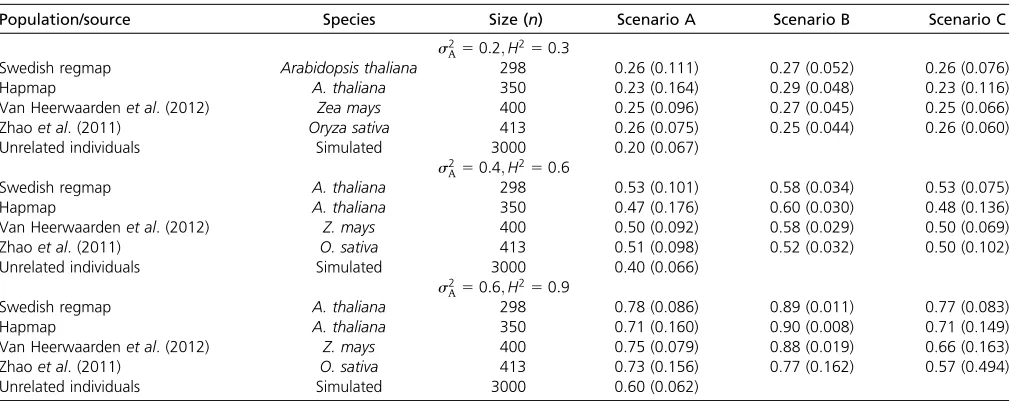
e s2

A ranges between 0.47 and 0.53, given a true value of 0.4 (Table 1). Similar bias occurs when s2

A50:2 and

s2

A 50:6: Hence, the presence of epistatic interactions leads to inﬂated estimates of additive genetic variance. For a panel of simulated unrelated individuals,se2Aequals the true value ofs2_A;_{which is due to the much smaller off-diagonal} elements ofK, makingKKalmost indistinguishable fromIn:

In scenario B, a plant trait is phenotyped onrgenetically identical replicates. Following Kruijeret al.(2015), the ob-servations Y5ðY11;. . .;YnrÞ9 are modeled by the normal

distribution

P_s2 A;s2E5N

0;s2_AZKZ9 1s2_EInr

; (2)

Zbeing an incidence matrix assigning plants to genotypes. The true distributionQis multivariate normal with covariance 0:4ZKZ9 10:2ZZ9 10:4Inr;i.e., there are nonadditive (not

necessarily epistatic) effects with independent Nð0;0:2Þ distributions. Such effects could be due to, for example, genotype–environment interaction. As in scenario A, we also consider a genetic architecture with h2₅₀_:_{2 and} H2₅₀_:_{3 (}_i.e._{, covariance 0}_:₂_ZKZ_{9 1}₀_:₁_ZZ_{9 1}₀_:₇_I

nr) and a

genetic architecture with h2₅₀_:_{6 and} _H2₅₀_:₉_:_In con-trast to model (1) (whereZ5Inandr51),ZZ9is different

fromInr;andQis not contained in model (2). Again, the

valuese2A minimizing KL divergence is substantially larger than the true value (Table 1), and additive genetic variance will tend to be overestimated. Intuitively, this is because the block structureZZ9is better captured byZKZ9than by the diagonal residual.

Scenario C is a combination of scenarios A and B. To avoid the misspeciﬁcation occurring in scenario B, the model

P_s2

A;s2G;s2E5N

0;s2AZKZ9 1s2GZZ9 1s2EIN

(3)

is considered, extending (2) with independent nonadditive effects. This model has been used in the analysis ofﬁeld trials (Oakey et al. 2006, 2007), as well as genomic prediction (Gianola and van Kaam 2008; Howard et al.2014; Jarquin et al.2014). If in fact the nonadditive effects have covariance KK(as in scenario A) ands2

A 50:4;the data have covari-ance 0:4ZKZ9 10:2ZðKKÞZ9 10:4Inr:As in scenarios A and

B, these2A minimizing KL divergence is larger than the true value (Table 1), except for the rice population of Zhaoet al. (2011) withH2₅₀_:₉_:_{In the latter case,}_e_s2

Ewas on average 0.14, while its bias was at most 0.01 for all other populations and heritability levels.

In addition to the minimization of KL divergence we analyzed ML estimates for simulated traits, in which case

Table 1 Values of the additive genetic varianceðse2

AÞminimizing the Kullback–Leibler divergence KL(Q, P) with respect to the true distribution (Q) of scenarios A–C, withPcontained in models (1)–(3)

Population/source Species Size (n) Scenario A Scenario B Scenario C

s2

A50:2;H250:3

Swedish regmap Arabidopsis thaliana 298 0.26 (0.111) 0.27 (0.052) 0.26 (0.076)

Hapmap A. thaliana 350 0.23 (0.164) 0.29 (0.048) 0.23 (0.116)

Van Heerwaardenet al. (2012) Zea mays 400 0.25 (0.096) 0.27 (0.045) 0.25 (0.066)

Zhaoet al. (2011) Oryza sativa 413 0.26 (0.075) 0.25 (0.044) 0.26 (0.060)

Unrelated individuals Simulated 3000 0.20 (0.067)

s2

A50:4;H250:6

Swedish regmap A. thaliana 298 0.53 (0.101) 0.58 (0.034) 0.53 (0.075)

Van Heerwaardenet al. (2012) Z. mays 400 0.50 (0.092) 0.58 (0.029) 0.50 (0.069)

Zhaoet al. (2011) O. sativa 413 0.51 (0.098) 0.52 (0.032) 0.50 (0.102)

s2

A50:6;H250:9

Swedish regmap A. thaliana 298 0.78 (0.086) 0.89 (0.011) 0.77 (0.083)

Van Heerwaardenet al. (2012) Z. mays 400 0.75 (0.079) 0.88 (0.019) 0.66 (0.163)

Zhaoet al. (2011) O. sativa 413 0.73 (0.156) 0.77 (0.162) 0.57 (0.494)

Minimization was performed by evaluating KL divergence on the grid 0, 0.01,. . ., 1 for all variance components, under the constraint they sum to one. Standard errors (in parentheses) were calculated as the square root of the asymptotic variance (White 1982, theorem 3.2). Five populations were considered: theArabidopsisHapmap and Swedish regmap (Hortonet al. 2012; Kruijeret al. 2015), the rice population from Zhaoet al. (2011), the maize population of van Heerwaardenet al. (2012), and a simulated population (File S1). In scenarios B and C there arer¼2 replicates of each genotype.

(3)

the phenotypic variance is unknown (File S2). For most populations and heritability levels, the bias of additive genetic variance estimates ðse2AÞ is similar to what was found by minimizing KL divergence in models (1)–(3). Differences are largest for the population of Zhao et al. (2011), where the total phenotypic variance is consis-tently overestimated.

The bias we identified here by statistical arguments and simulations has important implications, in particular for immortal populations, for which genetically identical rep-licates are available (e.g.,Arabidopsis thaliana, agronomic crops, bacteria, and fungi). Typically there is strong popu-lation structure and often only several hundreds of differ-ent genotypes are phenotyped. One can analyze such data at the individual level [model (2)] or at the level of geno-typic means [model (1), withs2_E’_{s divided by the number of} replicates]. Kruijeret al.(2015) showed that in the latter type of analysis, standard errors of heritability estimates can be huge, and recommended model (2) for both herita-bility estimation and genomic prediction. Here we have shown that in the presence of nonadditive effects, this model is likely to overestimate additive genetic variance. If, however, the nonadditive effects are due to epistatic interactions, analysis at the genotypic means level [model (1)] will, apart from the large sampling variance, also give inflated estimates of additive genetic variance. This is a rather realistic scenario, since epistasis may be an impor-tant part of the genetic architecture (Mackay 2014), and several other types of nonadditive effects can be ruled out or minimized for immortal populations: e.g., genotype– environment interactions are unlikely in homogeneous controlled environments with adequate randomization, and dominance effects are absent when using inbred lines. Inflated heritability estimates may also affect the perfor-mance of G-BLUP, although the loss in accuracy is consid-erably smaller than in the case where heritability is underestimated (Kruijeret al.2015).

Interestingly, the inflation of additive genetic variance is not due to any nonlinearity or absence of main effects (as in, e.g., Culverhouse et al.2002; Song et al. 2010; Zuket al. 2012), but rather to the population structure present in the epistatic GSM, which to some extent resembles the structure of the GSM for the additive effects. At the same time, it is this structure that makes the epistatic GSM distinguishable from the diagonal error. This suggests that epistatic interactions are easier to model in structured populations;i.e., sampling variance of epistatic variance components may not be as large as in unstructured human populations (Yang et al. 2011). Expressions for the asymptotic variance in a model with both additive and epistatic effects (File S3) indicate that this is indeed the case. More generally, the inflation of heritability estimates due to misspecification illustrates the difficulty of modeling and estimating genetic effects. As recently pointed out by Speed and Balding (2015) this is already challenging for the additive genetic effects, in the sense that depending on the genetic architecture, different GSMs may be appropriate.

Indeed, the potential bias resulting from an inappropriate GSM could be assessed by evaluating KL divergence with respect to the true model, as is the case for alternatives for the epistatic GSM considered here.

Acknowledgments

I thank two anonymous reviewers for their constructive comments that helped to improve the manuscript. Martin Boer and Fred van Eeuwijk are acknowledged for useful discussions. The research leading to these results has been conducted as part of the project DROught-tolerant yielding PlantS (DROPS), which received funding from the Euro-pean Community’s Seventh Framework Programme (FP7/ 2007-2013) under grant agreement 244374. This research was also funded by the Learning from Nature project of the Dutch Technology Foundation, which is part of the Nether-lands Organisation for Scientiﬁc Research.

Literature Cited

Culverhouse, R., B. K. Suarez, J. Lin, and T. Reich, 2002 A per-spective on epistasis: limits of models displaying no main effect. Am. J. Hum. Genet. 70: 461_–471.

Gianola, D., and J. B. C. H. M. van Kaam, 2008 Reproducing kernel Hilbert spaces regression methods for genomic assisted prediction of quantitative traits. Genetics 178: 2289_–2303. Horton, M. W., A. M. Hancock, Y. S. Huang, C. Toomajian, S. Atwell

et al., 2012 Genomewide patterns of genetic variation in worldwide Arabidopsis thaliana accessions from the RegMap panel. Nat. Genet. 44: 212–216.

Howard, R., A. L. Carriquiry, and W. D. Beavis, 2014 Parametric and nonparametric statistical methods for genomic selection of traits with additive and epistatic genetic architectures. G3 4: 1027–1046.

Huber, P. J., 1967 The behavior of maximum likelihood estimates under nonstandard conditions, pp. 221–233 inProceedings of the Fifth Berkeley Symposium on Mathematical Statistics and Proba-bility, Vol. 1. University of California Press, Berkeley, CA. Jarquin, D., J. Crossa, X. Lacaze, P. Du Cheyron, J. Daucourtet al.,

2014 A reaction norm model for genomic selection using high-dimensional genomic and environmental data. Theor. Appl. Genet. 127: 595_–607.

Jiang, Y., and J. C. Reif, 2015 Modelling epistasis in genomic selection. Genetics 201: 759_–768.

Kruijer, W., M. P. Boer, M. Malosetti, P. J. Flood, B. Engel et al., 2015 Marker-based estimation of heritability in immortal pop-ulations. Genetics 199: 379–398.

Lee, J. J., and C. C. Chow, 2014 Conditions for the validity of SNP-based heritability estimation. Hum. Genet. 133: 1011–1022. Mackay, T. F., 2014 Epistasis and quantitative traits: using model

organisms to study gene-gene interactions. Nat. Rev. Genet. 15: 22–33.

Oakey, H., A. Verbyla, W. Pitchford, B. Cullis, and H. Kuchel, 2006 Joint modeling of additive and non-additive genetic line effects in singleﬁeld trials. Theor. Appl. Genet. 113: 809–819. Oakey, H., A. Verbyla, B. Cullis, X. Wei, and W. Pitchford,

2007 Joint modeling of additive and non-additive (genetic line) effects in multi-environment trials. Theor. Appl. Genet. 114: 1319_–1332.

Song, Y. S., F. Wang, and M. Slatkin, 2010 General epistatic mod-els of the risk of complex diseases. Genetics 186: 1467_–1473.

(4)

Speed, D., and D. J. Balding, 2015 Relatedness in the post-genomic era: Is it still useful? Nat. Rev. Genet. 16: 33–44.

Speed, D., G. Hemani, M. R. Johnson, and D. J. Balding, 2012 Improved heritability estimation from genome-wide SNPs. Am. J. Hum. Genet. 91: 1011–1021.

van Heerwaarden, J., M. B. Hufford, and J. Ross-Ibarra, 2012 Historical genomics of North American maize. Proc. Natl. Acad. Sci. USA 109: 12420–12425.

Visscher, P. M., and M. E. Goddard, 2014 A general uniﬁed frame-work to assess the sampling variance of heritability estimates using pedigree or marker-based relationships. Genetics 199: 223_–232.

White, H., 1982 Maximum likelihood estimation of misspeci_ﬁed models. Econometrica 50: 1_–25.

Yang, J., B. Benyamin, B. P. McEvoy, S. Gordon, A. K. Henderset al., 2010 Common SNPs explain a large proportion of the herita-bility for human height. Nat. Genet. 42: 565–569.

Yang, J., S. H. Lee, M. E. Goddard, and P. M. Visscher, 2011 Gcta: a tool for genome-wide complex trait analysis. Am. J. Hum. Genet. 88: 76–82.

Zhao, K., C.-W. W. Tung, G. C. Eizenga, M. H. Wright, M. L. Aliet al., 2011 Genomewide association mapping reveals a rich genetic ar-chitecture of complex traits in Oryza sativa. Nat. Commun. 2: 467. Zuk, O., E. Hechter, S. R. Sunyaev, and E. S. Lander, 2012 The mystery of missing heritability: genetic interactions create phan-tom heritability. Proc. Natl. Acad. Sci. USA 109: 1193_–1198.

Communicating editor: A. H. Paterson

(5)

GENETICS

Supporting Information

www.genetics.org/lookup/suppl/doi:10.1534/genetics.115.177212/-/DC1

Misspeci

ﬁ

cation in Mixed-Model-Based Association Analysis

Willem Kruijer

(6)

File S1: simulation of unrelated individuals

Epistatic similarity matrices

Letzk = (zk,1, . . . , zk,n) (k= 1. . . , p) denote the vectors of standardized marker-scores for markersk= 1. . . , p. If we have corresponding marker effectssk ∼N(0, σA2/p), the resulting genetic similarity matrix has elements

Ki,j =p−1P p

k=1zk,izk,j =σA−2Cov( Pp

k=1skzk,i,P p

k=1skzk,j), for individualsi, j = 1, . . . , n. We extend this to an epistatic kernel as in [1] and [2], assuming independent epistatic effectsekl ∼N(0, σ2I/p

2_{) associated with}

the (entry-wise) productzkzl= (zk,1zl,1, . . . , zk,nzl,n). Assuming that the total genetic effect is

Ai+Ii= p X

k=1

skzk,i+ p X

k=1 p X

l=1

ekl(zk,izl,i), (1)

and independence of the additive and epistatic effects, it follows that Cov(Ai+Ii, Aj+Ij) =σ2AK+σI2(K·K), where K·K is the element-wise square (i.e. Hadamard product) ofK. In the model for the epistatic part we did not standardize (zkzl), which amounts to the assumption that bigger epistatic effects are expected for markers that are in LD. Finally, we note that equation (1) also contains termsekk (i.e. k =l), which, since there are already additive effects sk, could be interpreted as dominance effects. However, when the number of markerspis large, the contribution of these effects to the matrixK·Kis very small, as was shown in [3].

Simulation of unrelated individuals

We simulated 20000 bi-allelic SNPs in Hardy-Weinberg equilibrium. Minor allele frequencies were randomly drawn from the uniform distribution on [0.05,0.5]. No LD was simulated; although biologically unrealistic this is sufficient for our purpose, under the assumption that every causal variant is tagged by a SNP [4].

(7)

LITERATURE CITED LITERATURE CITED

Literature Cited

[1] Henderson C (1985) Best linear unbiased prediction of nonadditive genetic merits in noninbred populations. Journal of Animal Science : 111-117.

[2] Gianola D, de los Campos G (2008) Inferring genetic values for quantitative traits non-parametrically. Genetics Research 90: 525–540.

[3] Jiang Y, Reif JC (2015) Modelling epistasis in genomic selection. Genetics .

[4] Speed D, Hemani G, Johnson MR, Balding DJ (2012) Improved Heritability Estimation from Genome-wide SNPs. The American Journal of Human Genetics 91: 1011–1021.

(8)

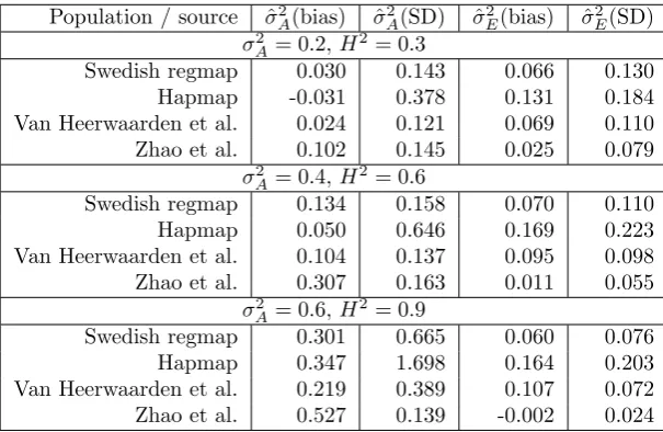
File S2: Simulations

We simulated phenotypic data given genotypic data, for the populations ofA. thaliana,Z. mays andO. sativa considered in the main text. For each population and scenario 5000 traits were simulated, following the dis-tributionsQof the scenarios A-C. Using the R packageasreml ([1]) we fitted respectively models 1-3 (see the main text). Bias and standard errors of the estimated variance components are given in Tables 1-3. In contrast to Table 1 in the main text, the total phenotypic variance is estimated from the data; hence the estimated bias of e.g. ˆσ2

A, ˆσG2 and ˆσ2E in Table 3 does not necessarily sum to 1.

Population / source σˆ2

A(bias) σˆ2A(SD) σˆE2(bias) σˆ2E(SD)

σ_A2 = 0.2,H2= 0.3

Swedish regmap 0.030 0.143 0.066 0.130

Hapmap -0.031 0.378 0.131 0.184

Van Heerwaarden et al. 0.024 0.121 0.069 0.110 Zhao et al. 0.102 0.145 0.025 0.079

σ_A2 = 0.4,H2= 0.6

Swedish regmap 0.134 0.158 0.070 0.110

Hapmap 0.050 0.646 0.169 0.223

σ2

A= 0.6,H 2_{= 0}_.₉

Swedish regmap 0.301 0.665 0.060 0.076

Hapmap 0.347 1.698 0.164 0.203

Van Heerwaarden et al. 0.219 0.389 0.107 0.072 Zhao et al. 0.527 0.139 -0.002 0.024

Table 1: Bias and standard deviation of estimates of additive genetic variance (σ2

A) and residual

variance (σ2

E) in scenario A, estimated from5000simulated traits. Phenotypic values were drawn from

the zero-mean normal distributions with covariance 0.2K+ 0.1(K·K) + 0.7In (top), 0.4K+ 0.2(K·K) + 0.4In

(middle), and 0.6K+ 0.3(K·K) + 0.1In (bottom). Estimates ˆσA2 and ˆσE2 were obtained by fitting model 1.

(9)

Population / source σˆ2

A(bias) σˆ2A(SD) σˆE2(bias) σˆ2E(SD)

σ_A2 = 0.2,H2= 0.3

Swedish regmap 0.094 0.069 0.012 0.055

Hapmap 0.095 0.060 0.007 0.053

σ_A2 = 0.4,H2= 0.6

Swedish regmap 0.228 0.083 0.006 0.032

Hapmap 0.216 0.068 0.002 0.030

σ2

A= 0.6,H 2_{= 0}_.₉

Swedish regmap 0.384 0.090 0.001 0.008

Hapmap 0.338 0.077 0.000 0.008

Van Heerwaarden et al. 0.413 0.082 0.001 0.007 Zhao et al. 0.521 0.100 -0.000 0.007

A) and residual

variance (σ2

E) in scenario B, estimated from5000 simulated traits withr= 2 replicates. Phenotypic

values were drawn from the zero-mean normal distributions with covariance 0.2ZKZ0+ 0.1ZZ0+ 0.7Inr (top),

0.4ZKZ0 + 0.2ZZ0+ 0.4Inr (middle) and 0.6ZKZ0+ 0.3ZZ0+ 0.1Inr (bottom). Estimates ˆσA2 and ˆσE2 were

obtained by fitting model 2.

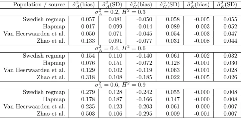
Population / source ˆσ2

A(bias) σˆ 2

A(SD) σˆ 2

G(bias) ˆσ 2

G(SD) σˆ 2

E(bias) ˆσ 2 E(SD)

σ2

A= 0.2,H2= 0.3

Swedish regmap 0.057 0.081 -0.050 0.058 -0.005 0.055

Hapmap 0.017 0.099 -0.014 0.089 -0.003 0.052

Van Heerwaarden et al. 0.050 0.071 -0.045 0.054 -0.003 0.047 Zhao et al. 0.133 0.091 -0.077 0.031 -0.008 0.044

σ_A2 = 0.4,H2= 0.6

Swedish regmap 0.154 0.110 -0.140 0.061 -0.002 0.032

Hapmap 0.076 0.151 -0.072 0.128 -0.001 0.030

σ_A2 = 0.6,H2= 0.9

Swedish regmap 0.279 0.128 -0.242 0.055 -0.000 0.008

Hapmap 0.178 0.187 -0.166 0.147 -0.000 0.008

A), non-additive

genetic variance (σ2

G) and residual variance (σ

2

E) in scenario C, estimated from 5000 simulated

traits with r= 2 replicates. Phenotypic values were drawn from the zero-mean normal distributions with

covariance 0.2ZKZ0+ 0.1Z(K·K)Z0+ 0.7Inr(top), 0.4ZKZ0+ 0.2Z(K·K)Z0+ 0.4Inr(middle) and 0.6ZKZ0+

0.3Z(K·K)Z0+ 0.1Inr (bottom). Estimates ˆσ2A, ˆσG2 and ˆσ2E were obtained by fitting model 3.

(10)

Literature Cited

[1] Butler DG, Cullis BR, Gilmour AR, Gogel BJ (2009) ASReml-R reference manual.

(11)

File S3: Asymptotic variance

Modeling non-additive genetic effects explicitly is known to be difficult, mainly because of the large sampling variance of the corresponding variance components [1]. This has motivated the use of non- and semi-parametric models, especially for genomic prediction [2]. In this supplement however we show that for the epistatic inter-actions, the sampling variance is considerably smaller for structured populations, compared to populations of unrelated individuals.

Suppose a single observation per genotype is available:

Yi=µ+Ai+Ii+Ei, (1)

where the vectors of additive (A) and epistatic effects (I) follow zero-mean multivariate normal distributions with covariance respectivelyσ_A2K and σ_I2(K·K). The matrix (K·K) is the Hadamard (entry-wise) product (see also File S1). The residual errorsEi have independent normal distributions with varianceσE2.

It follows from standard mixed model theory [3] that the REML estimators ˆσ_A2, ˆσ2_I and ˆσ_E2 based on this model are asymptotically unbiased, and Gaussian with covariance

Σˆσ2

A,σˆ

2

I,σˆ

2

E '2 



tr(P KP K) tr(P KP(K·K)) tr(P KP)

tr(P KP(K·K)) tr(P(K·K)P(K·K)) tr(P(K·K)P) tr(P KP) tr(P(K·K)P) tr(P P)



 −1

, (2)

whereP =V−1₋_V−1_X₍_Xt_V−1_X₎−1_Xt_V−1_,_X_{= 1}

nandV =σA2K+σ 2

I(K·K) +σ 2

EInis the covariance of the data. The asymptotic variance of ˆh2_{= ˆ}_σ2

A/(ˆσ2A+ ˆσI2+ ˆσ2E) can be obtained by application of the delta-method ([4]) to the function (σ2

A, σI2, σ2E)→σA2/(σ2A+σI2+σE2), which has gradient

bh2(σ_A2, σ_I2, σ2_E) =

_σ2

I +σE2 (σ2

A+σ 2 I +σ

2 E)2

, −σ

2 A (σ2

A+σ 2 I +σ

2 E)2

, −σ

2 A (σ2

A+σ 2 I+σ

2 E)2

.

Given the trueσ2

A,σ2I andσE2, it follows that

Var(ˆh2)'bh2(σ_A2, σ_I2, σ2_E) Σ_σ_ˆ2

A,σˆ2I,ˆσE2 b t

h2(σ2_A, σ2_I, σ_E2). (3)

Similar expressions can be derived for the proportions ˆσ_I2/(ˆσ_A2 + ˆσ2_I + ˆσ_E2) and ˆσ_E2/(ˆσ_A2 + ˆσ_I2+ ˆσ_E2). Because the matricesKand (K·K) have different singular value decompositions, it seems impossible to simplify these expressions in the same way as can be done for models with only additive effects [5]. We therefore evaluate the standard deviations numerically, for the 5 populations considered in the main text, and additionally the complete Arabidopsis regmap with 1307 accessions, and a subset of the simulated unrelated individuals of the same size (Table 1).

Population / source species size (n) SD(σ2

A/σ2) SD(σI2/σ2) SD(σE2/σ2)

Swedish regmap A. thaliana 298 0.227 0.269 0.130

Hapmap A. thaliana 350 0.220 0.298 0.242

Van Heerwaarden et al. Z. mays 400 0.147 0.175 0.119

Zhao et al. O. sativa 413 0.178 0.140 0.080

RegMap A. thaliana 1307 0.096 0.121 0.065

Unrelated individuals (subset) simulated 1307 0.153 1.897 1.898 Unrelated individuals simulated 3000 0.067 1.234 1.235

Table 1: Standard errors of the proportionsσˆ2_A/(ˆσ_A2+ ˆσ_I2+ ˆσ_E2),σˆ_I2/(ˆσ_A2+ ˆσ2_I+ ˆσ2_E)andσˆ2_E/(ˆσ2_A+ ˆσ_I2+ ˆσ_E2), based on the REML-estimators ˆσ_A2, σˆ_I2 and σˆ_E2 for model (1) defined above, and assuming that

σ2

A=σ 2

E = 0.4 and σ 2

I = 0.2. Seven populations were considered: the Arabidopsis Hapmap, Swedish regmap and complete regmap ([6], [7]), the rice population from [8], the maize population of [9] and two simulated populations.

Clearly, genetic relatedness leads to lower sampling variance of additive variance estimates, as was recently pointed out in [10]. For example, the standard error of narrow-sense heritability estimates is 0.153 for the simulated population with n = 1307, and 0.147 for the maize population of [9], with only 400 genotypes. Much larger differences occur for the proportion of phenotypic variance explained by epistatic interactions: for

(12)

unrelated individuals the epistatic similarity matrix (K·K) almost equals the identity, giving huge standard errors of both ˆσ_I2/(ˆσ_A2 + ˆσ_I2+ ˆσ2_E) and ˆσ_E2/(ˆσ_A2 + ˆσ_I2+ ˆσ2_E). These are much smaller for structured populations, although still considerable. Standard deviations may be further decreased when observations on genetically identical replicates are incorporated in the model, as in [7]; this is however beyond the scope of this work. Another possibility in that case is to extend the model with independent non-additive genetic effects, to model higher order interactions and/or other sources of non-additive genetic variance.

(13)

Literature Cited

[1] Yang J, Lee SH, Goddard ME, Visscher PM (2011) Gcta: A tool for genome-wide complex trait analysis. The American Journal of Human Genetics 88: 76 - 82.

[2] Gianola D, van Kaam JBCHM (2008) Reproducing kernel hilbert spaces regression methods for genomic assisted prediction of quantitative traits. Genetics 178: 2289-2303.

[3] Casella SRSG, McCulloch CE (2006) Variance components. Hoboken, NJ: John Wiley & Sons, xxiii + 501 pp.

[4] van der Vaart AW (2000) Asymptotic Statistics (Cambridge Series in Statistical and Probabilistic Mathe-matics). Cambridge University Press.

[5] Visscher PM, Goddard ME (2014) A general unified framework to assess the sampling variance of heri-tability estimates using pedigree or marker-based relationships. Genetics .

[6] Horton MW, Hancock AM, Huang YS, Toomajian C, Atwell S, et al. (2012) Genome-wide patterns of genetic variation in worldwide Arabidopsis thaliana accessions from the RegMap panel. Nat Genet 44: 212–216.

[7] Kruijer W, Boer MP, Malosetti M, Flood PJ, Engel B, et al. (2015) Marker-based estimation of heritability in immortal populations. Genetics 199: 379-398.

[8] Zhao K, Tung CWW, Eizenga GC, Wright MH, Ali ML, et al. (2011) Genome-wide association mapping reveals a rich genetic architecture of complex traits in Oryza sativa. Nature communications 2: 467+.

[9] van Heerwaarden J, Hufford MB, Ross-Ibarra J (2012) Historical genomics of north american maize. Pro-ceedings of the National Academy of Sciences .

[10] Speed D, Balding DJ (2015) Relatedness in the post-genomic era: is it still useful? Nature Reviews Genetics 16: 33–44.