Estimating Mutation Rate: How to Count Mutations?



Estimating Mutation Rate: How to Count Mutations?

Yun-Xin Fu

1

_{and Haying Huai}

Human Genetics Center, University of Texas, Houston, Texas 77030

Manuscript received August 28, 2002 Accepted for publication March 11, 2003

ABSTRACT

Mutation rate is an essential parameter in genetic research. Counting the number of mutant individuals provides information for a direct estimate of mutation rate. However, mutant individuals in the same family can share the same mutations due to premeiotic mutation events, so that the number of mutant individuals can be significantly larger than the number of mutation events observed. Since mutation rate is more closely related to the number of mutation events, whether one should count only independent mutation events or the number of mutants remains controversial. We show in this article that counting mutant individuals is a correct approach for estimating mutation rate, while counting only mutation events will result in underestimation. We also derived the variance of the mutation-rate estimate, which allows us to examine a number of important issues about the design of such experiments. The general strategy of such an experiment should be to sample as many families as possible and not to sample much more offspring per family than the reciprocal of the pairwise correlation coefficient within each family. To obtain a reasonably accurate estimate of mutation rate, the number of sampled families needs to be in the same or higher order of magnitude as the reciprocal of the mutation rate.

A

significant fraction of the genetic research of the direct estimate of the rate of mutation. These

experi-ments may be time consuming, but the statistical method last century has been to illuminate various aspects

of mutation (De Vries1901/1903;LuriaandDelbru¨ ck used for estimating mutation rate is straightforward and

should not be controversial. It appeared indeed to be

1943;McClintock1950;KeightleyandEyre-Walker

1999). This is natural because mutations are the ultimate the case for early geneticists (Bridges 1919; Wright

and Eaton 1926; Fisher 1930; Dobzhansky and source of genetic variation upon which natural selection

and other evolutionary forces can act (Kimura 1983; Wright1941). However, the increasing number of

ob-servations that some mutant offspring share the same

Lynch and Hill 1986; Johnson 1999). Early

experi-mutation has prompted many contemporary geneticists

ments on mutation rate include those byCastle(1905,

to reconsider how mutation rate should be estimated

1929),Muller(1920, 1928), andMorgan(1950). To

(Engels1979;RussellandRussell1996;Neel1998; date, extensive mutation data, from either mutation

Thompsonet al. 1998). experiments or surveys, are available for many species,

A clustered mutation means that two or more progeny

particularly fruit flies (Schalet1960;Crow and

Sim-of a family inherit the same mutation (Purdom et al.

mons1983), mice (FavorandNeuhauser-Klaus1994;

1968;HartlandGreen1970;FavorandNeuhauser

-Russelland Russell1996), and humans (Neel and

Klaus 1994). Mutation clusters have been widely

ob-Rothman 1978; Cooper and Krawczak 1993; Crow

served and are now considered as general rather than 1993, 1999). Due to the importance of mutation rate,

as the exception (Hall 1988; Drost and Lee 1995;

such experiments will be likely to continue in the future,

MohrenweiserandZingg1995;HuaiandWoodruff

with more and more details being revealed by the advent

1997; Paashuis-Lew and Heddle 1998; Lewis 1999;

of new molecular techniques (KondrashovandCrow

for reference, see Woodruff et al. 1996). The most

1993;Fu1994).

important issue created by mutation cluster is how to In a typical mutation experiment, some aspects of the

count the mutations for the purpose of estimating muta-progeny of well-characterized parents are examined. A

tion rate. Several ways of counting have been proposed. mutant is identified if an offspring differs from its

par-One is to count each mutant offspring as one mutation, ents in a way that can be explained only by invoking a

disregarding whether or not the mutation is shared

mutation (Auerbach1959;Drake1991, 1993). When

(Haldane1935;SpencerandStern1948;Auerbach

a large number of offspring of mating pairs have been

1962; Muller et al. 1963; Combes et al. 1989; Huai

examined, the proportion of mutant progeny yields a

1997). The second is to count each cluster as only one

mutation (Russell 1977;Shukla et al. 1979; Heddle

et al. 1996; Nishinoet al. 1996). The third is to count

1_{Corresponding author:Human Genetics Center, SPH, University of}

only those mutations that are not clustered (

Abra-Texas, 1200 Herman Pressler, Houston, TX 77030.

E-mail: [email protected] hamsonandWolff1976;RussellandRussell1992),

but in many cases this third choice is made because only the induced mutations in limited stages of the life

cycle are measured (Masonet al. 1987;Arraultet al.

2002). Various arguments have been put forward to

support one method or the other (RussellandRussell

1992, 1996; Huai and Woodruff 1998a,b; Heddle

1999), but no resolution has been obtained to date (Thompsonet al. 1998;StuartandGlickman 2000). In this article, we show for the first time that counting each mutant as one mutation regardless of cluster is the correct way to obtain an unbiased estimate of the mutation rate. Of equal significance is the formula for the sampling variance of the estimator, which does not require knowing all family sizes. We also discuss two important issues in designing a mutagenesis experi-ment, the sampling strategy and sample size

require-Figure1.—An example of mutations and their relationships

ment. Furthermore, we reanalyze several large data sets

withhiandmj. and show that some of the results in mutation rate

estimates have an undesirably large variance.

The equivalence of this counting to that of Equation

THEORY

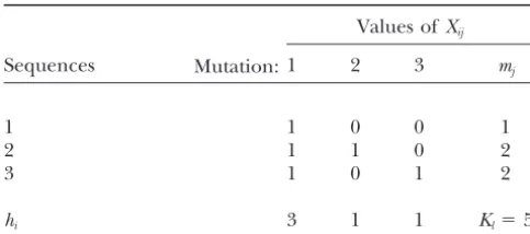
1 can be proved as follows. LetXijbe the index variable

Counting mutations: Suppose a total of m haploid _{that takes value 1 if theith mutation is inherited by the}

families are studied in an experiment. Let ni be the _{jth sequence and value 0 otherwise. Figure 1 (see Table}

number of offspring examined in theith family andn⫽ _{1 also) gives an example, from which we can easily see}

n1⫹. . .⫹nmbe total sample size. Considering thelth _{the relationship betweenX}

ijandhi andmjas family, an individual is a mutant if it differs from its

parent(s) by at least one mutation. It is important to _{hi ⫽Xi1⫹. . . ⫹Xin}

l (5)

realize that mutations in different mutant individuals

mj⫽X1j⫹. . . ⫹XIj. (6)

are not necessarily distinct. LetKlbe the total number

of mutations counted as follows: each mutation that is

It follows that

inherited bykindividuals (more preciselyksequences)

is countedktimes. That is, suppose that there are in total _K

l⫽h1 ⫹. . .⫹ hI

I independent mutation events, and the ith mutation

is inherited byhisequences. Then _⫽

兺

I

i⫽1

兺

n_l

j⫽1

xij

Kl⫽h1⫹. . . ⫹hI. (1)

⫽

_兺

nl

j⫽1

兺

I

i⫽1

xij Note that if there is only one mutant for each mutation

event,Kis simply the number of mutant individuals.

The total number of mutations in the experiment is ⫽m1⫹m2⫹. . . ⫹mn_l.

defined as (7)

One special case deserves mentioning. When only

K⫽K1⫹. . . ⫹Km. (2)

one sequence is examined per family, each mutation

event will be counted exactly once. Therefore, K in

A mutation is said to be size iif there arei mutants

in the sample sharing that mutation. Letclbe the num- this situation is equal to the number of independent

ber of clusters of mutations of sizel. Then it is easy to mutations in the experiment.

see that RepresentingKby Equation 4 provides a convenient

basis for studying its statistical properties, and we discuss

K⫽c1⫹2c2⫹ . . .⫹ LcL, (3)

the mean and variance below.

whereLis the maximum cluster size. The mean and variance of K: Let R represent the

Consider thelth family again. Although Equation 1 number of DNA replications between two successive

indicates thatKis counted by considering each muta- _{generations and␯ibe the mutation rate for theith cell}

tion at a time, it can also be counted by considering _{replication. Let}

one sequence at a time. Letmjbe the number of

muta-␮i⫽ ␯1⫹. . . ⫹ ␯i. (8)

tions that occurred in individual (sequence)j. Then

TABLE 1

An example of mutations and their relationships with

hiandmjas shown in Figure 1

Values ofXij

Sequences Mutation:1 2 3 mj

1 1 0 0 1

2 1 1 0 2

3 1 0 1 2

hi 3 1 1 Kl⫽5

sequence (Figure 2). We assume thatRis a fixed number, _{Figure2.—Relationship between two sequences in a family.}

which is appropriate for experiments in which individuals sampled are of the same sex and about the same age.

We assume that the number of mutations at

replica-tionifollows the Poisson distribution with both mean _{fore, whether a single gene is considered or multiple}

and variance of␯i. Thus for anyjsequence overRinde- genes are pooled,␮ˆ is an unbiased estimator of␮.

pendent cell divisions, _{We now consider the variance of␮ˆ . Consider first the}

case in whichnl⫽1 for alli. As we mentioned earlier,

E(mj)⫽ Var(mj)⫽ ␮, (9)

Kis equivalent to the number of mutation events. Since

the mutations in different families are independent, we

whereE( ) and Var( ) stand for expectation and

vari-have ance, respectively. We also assume that mutations in

different families are independent.

Var(K)⫽

兺

l

Var(Kl)⫽n␮. (13)

Since

E(Kl)⫽

兺

E(mj) (10) Therefore

⫽nl␮, Var(␮_{ˆ )}⫽ Var(_k)/_n2 ⫽ ␮/_n. (14)

it follows that _{In general, we have}

E(K)⫽

兺

l

E(Kl) _Var(K

i)⫽

兺

Var(mi)⫹

兺

i⬍j

Cov(mi,mj)

⫽ ␮

_兺

l

nl ⫽_n␮ ⫹ φ

兺

l

nl(nl ⫺1) , (15)

⫽n␮. (11)

where

This equation suggests that an unbiased estimator of␮is _φ⫽

Cov(mi,mj) .

␮ˆ ⫽ K/n, (12)

So φis the covariance between mi and mj, that is, the

covariance of the numbers of mutations in any pair of which is exactly the way the mutation rate has been

sequences from the same family. Therefore

estimated in some empirical studies (e.g., Haldane

1935; Spencer and Stern 1948; Auerbach 1962;

Var(K)⫽n␮ ⫹ ␳␮

兺

l

nl(nl⫺ 1) .

Muller et al. 1963; Woodruff and Thompson 1992;

Huai1997; Drakeet al. 1998;Thompsonet al. 1998).

And then Counting each cluster as one mutation or counting only

independent mutations will result in underestimation

Var(␮ˆ )⫽ ␮

n ⫹ ␳␮

兺

lnl(nl⫺ 1)

n2 , (16)

of the true mutation rate; in some cases the

underesti-mation may well be a few fold (Paashuis-Lewand

Hed-dle1998;Selby1998a,b;Thompsonet al. 1998;Heddle where ␳ ⫽φ/␮ is the correlation coefficient between

the numbers of mutations in two different sequences

1999). Since the mutation rate␮in this article is defined

as the sum of mutation rates over cell replications that from the same family.

Two special cases are illuminating. The first is that

are not necessarily equal, it does not matter if␮

exam-ined,i.e.,nl⫽c,l⫽1,. . .,m. It follows from Equation it is thus the proportion of mutations that are shared by two sequences from the same family.

16 that

Let rl,ij be the number of shared mutations for

se-Kl⫽K/(mc)

quencesiandjin thelth family. It thus follows that

and

E[rl,ij]⫽ ␮ E(t)

␮ . (27)

Var(␮ˆ )⫽ 1

m

冢

1

c ⫹ ␳ c ⫺1

c

冣

␮. (17)

The above equation suggests that an unbiased

estima-The second case is that all the offspring of each family tor of␮E(t)is

are examined. Since offspring number of a family is

typically not a predetermined quantity, we have _␮ˆE(t)⫽

2

兺

lnl(nl⫺1)

兺

l

兺

i⬍j

rl,ij, (28)

E(K)⫽ ␮

兺

E(nl) (18)

wherenl(nl⫺1)/2 is the number of pairs of sequences

Var(K)⫽ ␮

兺

E(nl)⫹φ

兺

E[nl(nl⫺ 1)]. (19)

for all the sample from the lth family. Suppose that

The most common practice is to assume that offspring _{there are in totalLobserved clusters and c}

i is the size

number of a family follows a Poisson distribution with _{of clusteri. The above estimator can then be written as}

meanf. Then

␮ˆE(t)⫽

兺

L

i⫽1ci(ci⫺ 1)

兺

lnl(nl⫺1)

. (29)

E(K)⫽mE(Kl)⫽ mf␮ (20)

Var(K)⫽mVar(Kl)⫽mf␮ ⫹mφf2. (21)

Substituting this into Equation 16 yields an unbiased

estimate of the standard error of␮ˆ as

So we have

␴ˆ ⫽ 1

n

冪

K⫹

兺

L

i⫽1

ci(ci⫺1) . (30)

Var(␮ˆ )⫽ 1

m

冢

1

f ⫹ ␳

冣

␮. (22)

Estimating the sampling variance:Since␮ˆ is an unbi- Since many experiments on mutation rate were done

ased estimator, the precision of estimation is thus deter- over the many decades, detailed cluster sizes may not

mined by its variance. To compute the variance of␮ˆ , be available. So the above formula is difficult to apply

we need to know the value of the covariance between in many situations. However, boundaries of the standard

two mutations (see Figure 2). error of␮ˆ can be obtained on the basis of partial

infor-Suppose that sequence i and sequence j shared a mation as follows.

common ancestortcell replications ago. Then we can If only the numberSof singletonsLandKis known,

expressmiandmjas then the minimum value attainable by兺c_i(c_i⫺1) is (K⫺

S)(K ⫺ S ⫺ L)/L, corresponding to the situation in

mi⫽ rij⫹ri (23)

which all clusters are of equal size (K⫺S)/L. A

lower-mj⫽ rij⫹rj, (24) bound of the standard error is thus given by

where rij represents the number of mutations in the

␴min⫽

1

n

冪

K⫹

(K⫺S)(K⫺S⫺L)

L . (31)

common ancestor (shared mutations), andriandrjare

the numbers of mutations in sequencesiandj,

respec-Letcminandcmaxbe the minimum and maximum

clus-tively, since the separation from their common ancestor

ter sizes, respectively. Then we have 2ⱕ cmin ⱕ cmax ⱕ

(Figure 2). Conditional on thetvalue,rij,ri, andrjare

K⫺S⫺cmin(L⫺1). The maximum value of兺ci(ci⫺ 1)

independent Poisson variable with means equal to ␮t,

corresponds to the situation in which there are as many

␮ ⫺ ␮t, and␮ ⫺ ␮t, respectively. Therefore

clusters ofcminsize as possible. An upper bound of the

E(mimj)⫽ Et[E(r2ij ⫹rij(ri⫹ rj)⫹ rirj)]

standard error is therefore given by

⫽ Et[␮t⫹ ␮2t ⫹2␮t(␮ ⫺ ␮t)⫹(␮ ⫺ ␮t)2]

␴max⫽

1

n

√

K⫹cmin(L⫺b)⫹ bcmax(cmax ⫺1) , (32)

⫽ Et[␮t⫹ ␮2]

⫽ ␮E(t)⫹ ␮2. (25) whereb ⫽(K⫺ S⫺c_minL)/(c_max⫺c_min).

We can also construct a confidence interval for

esti-It follows thatφ⫽E(mimj)⫺E(mi)E(mj)⫽ ␮E(t). Soφis

mating␮ˆ . Note that␮ˆ is the average of many variables

the expected number of shared mutations between two

with the same mean and variance and 0 or small covari-sequences from the same family. Since the correlation

ance; therefore, by the central limit theorem of

proba-coefficient␳is defined as

bility,␮ˆ can be approximated by a normal distribution

with mean␮and variance␴2_{. The 95% confidence}

inter-␳ ⫽ ␮E(t)

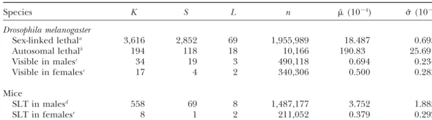
TABLE 2

Examples of estimates of mutation rate and standard error

Species K S L n ␮ˆ (10⫺4₎ ␴_{ˆ (10}⫺4₎

Drosophila melanogaster

Sex-linked lethala _{3,616 2,852 69 1,955,989 18.487 0.695}

Autosomal lethalb _{194 118 18 10,166 190.83 25.69}

Visible in malesc _{34 19 3 490,118 0.694 0.234}

Visible in femalesc _{17 4 2 340,306 0.500 0.283}

Mice

SLT in malesd _{558 69 8 1,487,177 3.752 1.885}

SLT in femalese _{8 1 2 211,052 0.379 0.292}

a_{Details in tables ofMasonet al. (1985) andWoodruffandThompson(1992).}

b_{Details inSchalet(1960),Shuklaet al. (1979),Woodruffet al. (1996), and also in Table 3 ofThompson} et al. (1998).

c_{Schalet(1960) andShuklaet al. (1979); see also Table 3 ofThompsonet al. (1998).}

d_{FavorandNeuhauser-Klaus (1994),Russelland Russell (1996),Drostand Lee (1995, 1998), and}

Selby (1998a,b).

e_{Russell(1964),RussellandRussell (1992), andSelby (1998a,b).}

Even though the mutation rate estimates of male and assumption of Bernoulli (Poisson) distribution due to

premeiotic mutation events. Even though his formulas female mice have a not so small variance, we note that

the mean ratio of the mutation rate estimates of mouse appear to be more influential than Muller’s, especially

in Drosophila mutagenesis involving transposable ele-males over mouse feele-males is 10 in Table 2, compared

to the value of 2 in Changet al. (1994). The sample ments (Margulieset al. 1986;EhlingandNeuhauser

-Klaus1988;Brownet al. 1989;BadgeandBrookfield

size for female mice in the specific locus test (SLT) is

far below that for male mice. Thus cluster mutations in 1998), most of his conclusions and parameter

estima-tions are not relevant to the premeiotic cluster muta-female mice may well be underestimated or not

recov-ered. More experiments are needed for a specific locus tions.

Sampling strategy: Since ␮ˆ is an unbiased estimator test of female mice.

of␮, sampling strategy should aim at reducing the

vari-ance of the estimate. When to sample and how to sample both play important roles in determining the variance.

DISCUSSION

Before we examine these two issues in turn, we note

Relation to others’ work:Muller(1952, 1962)

pre-that the best possible strategy is to examine as many

sented an estimator of the standard error of␮ˆ as␴ˆ ⫽ _{families as possible but only one sequence per family.}

q(1/n)

√

兺L

i⫽1ci(ci⫺1) (q ⫽ 1 ⫺ ␮ˆ , and singletons are _{This sampling strategy will minimize the sampling}

vari-considered as special cases of cluster mutations), which _{ance for a fixed total number of individuals examined}

is close to but tends to underestimate␴ˆ compared with _{(compare Equation 13 with Equation 16). Apparently}

Equation 30 of this article. The derivation of this for- _{this strategy is neither practical in most situations for}

mula was never given, but Muller appeared to have _{multicellular organisms nor possible in somatic or}

bacte-obtained this formula with the assumption that the pre- _{ria mutagenesis (LuriaandDelbru¨ ck1943; Heddle}

meiotic mutations are not common; his brief explana- _{1999; H.Huaiand Y.-X.Fu, unpublished results). There}

tion of the formulas suggested that it may be the result _{are good reasons for choosing large family sizes in}

cer-of a compound or generalized Poisson process, which _{tain situations. For example, it is important to know}

is the sum of independent Poisson variables. _{the value of ␳ for the purpose of understanding the}

Engels(1979) also gave formulas for both mean and _{clustering phenomenon of mutations, and ␳ can be}

variance of mutation rates when cluster mutations are estimated better with larger family sizes. Another reason

present. He focused mainly on a clustering model vio- favoring larger family size is that there may be a nearly

lating homogeneity of mutation probabilities among fixed amount of effort or expense for each family

different parents. Engels visualized a conceptual two- screened regardless of its size.

step experiment. The first step consists of choosing from It is clear from the variance equation (16) that the

a pool of possible mutation rates for all different par- best sampling time is the one that minimizes the

correla-ents. The second step is the independent Bernoulli sam- tion coefficient␳between any pair of progeny within a

pling within each family. So Engels did not address family. Apparently, this indicates that the best time to

TABLE 3

The variation coefficient␣(␣⫽␴ˆ /␮ˆ ) when all themfamilies are of the same sizefand when␳⫽0.10

Family size (f)

m⫻u 1 5 10 50 100 1,000 10,000

0.01 10.000 5.292 4.359 3.435 3.302 3.176 3.164

0.1 3.162 1.673 1.378 1.086 1.044 1.004 1.000

1 1.000 0.529 0.436 0.344 0.330 0.318 0.316

3 0.577 0.306 0.252 0.198 0.191 0.183 0.183

10 0.316 0.167 0.138 0.109 0.104 0.100 0.100

tion in multicellular species when germ cell number is f (orcmax)Ⰷ ␳⫺1, the further increase of mean family

size does not help to reduce the variance much (see small. Also note that males, especially older males in

many species, usually have much more germ cell divi- Table 3 and Figure 3). Therefore a reasonable strategy

is to examine as many progeny per family as possible sions than females have; hence it may be possible that

the correlation coefficients␳are much lower in males, but not much more than␳⫺1_.

Because of the important role of␳in the estimate of

especially in older males.

Given that the sampling time is determined, that is, mutation rate and genetic counseling (Hartl 1971;

Wijsman 1991; Young1991), it is useful to obtain an

␳ is fixed, how many individuals to sample from each

family depends on the value of␳. To demonstrate, con- estimate of ␳ from experimental data (Van Essen et

al. 1992; CooperandKrawczak 1993;Bridges1994;

sider the case wherenl⫽cmax⫽f,l⫽1, . . . ,mor that

family size follows Poisson distribution. We note from Zlotogora1998). From Equation 29, we can estimate

␮ˆE(t)by

both Equations 17 and 22 that the variance of the esti-mate of mutation rate is approaching

␮ˆE(t)⫽

兺

L

i⫽1ci(ci⫺ 1)

(m⫺1)␴2

f ⫹n(f⫺1)

, (34)

1

m␮ˆE(t) (33)

where fis the mean family size and␴2

f is the sampling

variance of the family size,i.e.,

with an increasing and large enough family size. Once

a useful experiment for estimating mutation rate should

␴2

f ⫽ 1

m⫺ 1

兺

i

(ni⫺ f)2 (35)

examine at least as many families as the reciprocal of the mutation rate (Table 3, Figures 3 and 4). This con-clusion will reintroduce the problem of how to avoid

⬇ 1

m

兺

i

n2

i ⫺f2. (36)

preexisting mutations if the sampled family number is at least as large as the reciprocal of the mutation rate.

So ␳can be estimated by

Can we find a way that de novocluster mutations can

be discriminated confidently from preexisting

muta-␳ ⫽ ␮E(t)

␮ tions? It is relatively easy to eliminate the preexisting

mutations that are from grandparents’ heterozygosity (Yang et al. 2001), but if one of the grandparents is

⫽ n

兺

L

i⫽1ci(ci⫺1)

K[(m⫺1)␴2

f ⫹n(f⫺ 1)]

(37)

genetic mosaic for a new mutation, then we need careful

analysis of its timing and effects (H.Huaiand Y.-X.Fu,

unpublished results).

⬇

兺

Li⫽1ci(ci⫺1)

K(␴2

f/f⫹f)

. (38)

Estimating ␮ from the number of mutation events:

Let Ibe the number of mutation events in an

experi-Kis the total number of mutants recovered in the

ex-ment that examinedsoffspring. As we have shown, when

periment, counting all members of any clusters.

one sequence is examined per family,Iis the same as

Sample size requirement: Besides sampling strategy

Kso usingI/syields an unbiased estimate of␮. When

to reduce variance in the estimate, it is important to

multiple offspring from a family are examined, I can

determine the sample size required in achieving a given

be ⬍K; the magnitude of difference depends on the

precision in estimation. It is obvious that the standard

number of offspring examined as well as on␮ˆE(t).

error of an estimate should not be larger than the

esti-SinceK/nis an unbiased estimate of␮, it follows that

mate itself. For a good estimate, the standard error

I/nis an underestimate of mutation rate. It is tempting

should probably be an order of magnitude smaller than

to suggest an estimate as the estimate.

Kl ⫽I/n⬘, (41) For simplicity, consider the case that an equal number

of progeny is examined for each family. Suppose we

wheren⬘is a constant satisfyingmⱕn⬘ ⬍n. However,

want to ensure that the standard error is as small as␣␮. _{it is not obvious what valuen⬘should be. Hence}

count-Then family numbermand family size f(cmax) need to _{ing each mutant as one mutation regardless of the}

clus-satisfy _{ter’s origin is the more straightforward way to obtain}

an unbiased estimate of the mutation rate. Nevertheless, 1

m

冢

1

f ⫹ ␳ f⫺ 1

f

冣

␮ ⫽ ␣

2␮2 ₍₃₉₎

it should be worth exploring efficient ways to use the frequencies of various mutation events.

Alternative ways to combine information: We note or

thatKl/nlis an unbiased estimate of␮. So

m⫽ ␣⫺2␮⫺1

冢

1

f ⫹ ␳ f⫺ 1

f

冣

. (40) ␮ˆ⬘ ⫽

兺

_i␤iKl/nl (42)

is an unbiased estimator, where ␤i ⱖ 0 and 兺i␤i ⫽ 1.

We can see from Table 3 and Figure 3 that it is obvious

Because

that once the uniformly sampled family sizefis above

the reciprocal of␳, further increases offwill not help _{Var(␮ˆ⬘)⫽}

_兺

i (␤2

i/nl)(␮ ⫹ ␮E(t)(nl⫺1)) , (43) reduce the standard error of mutation rate estimation

very much. In these cases there is an optimum family

to obtain a best linear estimate of␮,␤needs to satisfy

size (a little bit ⬎␳⫺1_{) at which the experiment is most}

efficient. So it is not always true that the larger the _2␤

i

ni(␮ ⫹ ␮E(t)(ni⫺1))

⫽ 2␤m

nm(␮ ⫹ ␮E(t)(nm⫺1))

, (44)

sample size, the more precise the experiment.

On the other hand, given that the total sample size

wherei⫽1, . . . ,m⫺1. That is,

is fixed (shown in Figure 4), the best sampling strategy

is to examine as many families as possible where the _␤

i

␤m

⫽ ni(␮ ⫹ ␮E(t)(ni⫺ 1))

nm(␮ ⫹ ␮E(t)(nm⫺1))

. (45)

family sizefis fixed at one, where each sample is

inde-pendent from others. If this is not feasible, try to fix

So the family size as low as possible when there is no need

for estimation of␳.

␤i⫽

冢

兺

i

ni

1⫹ ␳(ni⫺1)

冣

⫺1

ni

1⫹ ␳(ni⫺1)

. (46)

Also family size f can affect the number of families

that need to be studied, but the most important factor

Figure4.—The total sample size fixed at

m⫻f⫽100/␮, and all themfamilies are of the same sizef. The designed family sizes vary from 1.0 to 1000 to visualize their ef-fects on the variation coefficient of muta-tion rate estimamuta-tion.

Combes, R. D., J. Bootman, M. G. Ford, J. HepworthandD. W. combine data from different families is to give each

Salt, 1989 Statistical method for the design and analysis of

individual equal weight regardless of family affiliation, _{mutation experiments with the fruit flyDrosophila melanogaster, pp.}

251–283 inStatistical Evaluation of Mutagenicity Test Data, edited by because each provides the same amount of independent

D. J.Kirkland. Cambridge University Press, Cambridge, UK.

information; when␳is close to one, the best way is to

Cooper, D. N., andM. Krawczak, 1993 Human Gene Mutation. BIOS

give equal weight to each family, because each family _{Scientific Publishers, Oxford.}

Crow, J. F., 1993 How much do we know about spontaneous human provides the same amount of information regardless of

mutation rates? Environ. Mol. Mutagen.21:122–129. size.

Crow, J. F., 1999 Spontaneous mutation in man. Mutat. Res.437: 5–9.

This work was supported in part by National Institutes of Health

Crow, J. F., andM. J. Simmons, 1983 The mutation load in Drosoph-grants R29 GM50428 (Y.X.F.) and R01 HGO1708 (Y.X.F.).

ila, pp. 1–35 inThe Genetics and Biology of Drosophila, Vol. 3c, edited by M.Ashburner, H. L.Carsonand J. N.Thompson. Academic Press, London.

De Vries, H., 1901/1903 Die Mutations Theorie, Vols. 1 and 2, Veit,

LITERATURE CITED

Leipzig, Germany (English translation, 1909/1910. Open Court, Abrahamson, S., and S. Wolff, 1976 Re-analysis of radiation- _Chicago).

induced specific locus mutations in mouse. Nature264:715–719. _{Dobzhansky,T. H., and S.Wright, 1941 Genetics of natural} popu-Arrault, X., V. Michel, P. Quillardet, M. HofnungandE. Touati, _{lations. V. Relations between mutation, rate and accumulation} 2002 Comparison of kinetics of induction of DNA adducts and _{of lethals in populations ofDrosophila pseudoobscura. Genetics26:} gene mutations by a nitrofuran compound, 7-methoxy-2-nitro- _23–51.

naphtho[2,1-b]furan (R7000), in the caecum and small intestine _{Drake, J. W., 1991 Spontaneous mutation. Annu. Rev. Genet.25:}

of Big BlueTM mice. Mutagenesis17:353–359. _125–146.

Auerbach, C., 1959 Spontaneous mutations in dry spores of Neuro- Drake, J. W., 1993 Rates of spontaneous mutation among RNA

spora crassa. Z. Vererbungsl.90:335–346. _{viruses. Proc. Natl. Acad. Sci. USA90:4171–4175.}

Auerbach, C., 1962 Mutation: An Introduction to Research in Mutagene- Drake, J. W., B. Charlesworth, D. CharlesworthandJ. F. Crow,

sis. Part I. Methods.Oliver & Boyd, Edinburgh. 1998 Rates of spontaneous mutation. Genetics148:1667–1686. Badge, R. M., andJ. F. Y. Brookfield, 1998 A novel repressor of _{Drost, J. B}., andW. R. Lee, 1995 Biological basis of germline muta-P-element transposition inDrosophila melanogaster.Genet. Res.71: tion: comparisons of spontaneous germline mutation rates

21–30. among Drosophila, mouse, and human. Environ. Mol. Mutagen.

Bridges, C. B., 1919 The stages at which mutations occur in the 25(Suppl. 26): 48–64.

germ tract. Proc. Soc. Exp. Biol. Mod.17:1–2. Drost, J. B., and W. R. Lee, 1998 The developmental basis for

Bridges, P. J., 1994 The Calculation of Genetic Risks. Johns Hopkins the germline mosaicism in mouse andDrosophila melanogaster.

University Press, Baltimore. Genetica102/103:421–443.

Brown, A. J. L., L. S. Alphey, A. J. Flavell, T. I. Gerasimovaand Ehling, U. H., andA. Neuhauser-Klaus, 1988 Induction of spe-S. J. Ross, 1989 Instability in the Ctmr2 strain of Drosophila cific-locus and dominant-lethal mutations by cyclophosphamide

melanogaster: role of P-element functions and structure of re- and combined cyclophosphamide-radiation treatment in

male-vertants. Mol. Gen. Genet.218:208–213. mice. Mutat. Res.199:21–30.

Castle, W. E., 1905 The mutation theory of organic evolution: from Engels, W. R., 1979 The estimation of mutation rates when premei-the standpoint of animal breeding. Science21:521–525. otic events are involved. Environ. Mutagen.1:37–43.

Castle, W. E., 1929 A mosaic(intense-dilute) coat pattern in the Favor, J., and A. Neuhauser-Klaus, 1994 Genetic mosaicism in the house mouse. Annu. Rev. Genet.28:27–47.

Fisher, R. A., 1930 Note on a tricolour (mosaic) mouse. J. Genet. Radiosensitivity in Germ Cells, edited byF. Sobels. Pergamon Press,

23:77–81. Oxford.

Fu, Y. X., 1994 A phylogenetic estimator of population size or muta- Neel, J. V., 1998 A reappraisal of studies concerning the genetic

tion rate. Genetics136:685–692. effects of the radiation of humans, mice, and Drosophila. Environ.

Haldane, J. B. S., 1935 The rate of spontaneous mutation in a Mol. Mutagen.31:4–10.

human gene. J. Genet.31:317–326. Neel, J. V., andE. D. Rothman, 1978 Indirect estimates of mutation

Hall, J. G., 1988 Somatic mosaicism: observations related to clinical rates in tribal Amerindians. Proc. Natl. Acad. Sci. USA75:5585–

genetics. Am. J. Hum. Genet.46:1187–1193. 5588.

Heddle, J. A., 1999 On clonal expansion and its effects on mutant Nishino, H., D. J. Schaid, V. L. Buettner, J. HaavikandS. Sommer, frequencies, mutation spectra and statistics for somatic mutations 1996 Mutation frequencies but not mutant frequencies in big

in vivo. Mutagenesis14:257–260. blue mice fit a Poisson distribution. Environ. Mol. Mutagen.28:

Heddle, J. A., L. Cosentino, G. Dawood, R. R. SwigerandY. Paas- 414–417.

huis-Lew, 1996 Why do stem cells exist? Environ. Mol. Muta- Paashuis-Lew, Y. R. M., andJ. A. Heddle, 1998 Rates of mutation

gen.28:334–341. during embryogenesis and growth. Mutagenesis13:613–617.

Hartl, D. L., 1971 Recurrence risks for germinal mosaics. Am. J. Purdom, C. C., K. F. DyerandD. G. Papworth, 1968 Allelic clusters

Hum. Genet.23:124–134. among spontaneous mutations in Drosophila. Mutat. Res.5:305–

Hartl, D. L., andM. M. Green, 1970 Genetic studies of germinal 307. mosaicism inDrosophila melanogasterusing the mutablewc_gene.

Russell, L. B.,1964 Genetic and functional mosaicism in the mouse,

Genetics65:449–456. _{pp. 153–181 inThe Role of Chromosomes in Development, edited by}

Huai, H., 1997 The evolutionary implication of premeiotic clusters _{M. Locke. Academic Press, New York.}

of mutation. Ph.D. Thesis, Bowling Green State University, Bowl- _{Russell, L. B., andW. L. Russell, 1992 Frequency and nature of}

ing Green, OH. _{specific-locus mutations induced in female mice by radiation and}

Huai, H., andR. C. Woodruff, 1997 Clusters of identical new muta- _{chemical: a review. Mutat. Res.296:107–127.}

tions can account for the “overdispersed” molecular clock. Genet- _{Russell, L. B., andW. L. Russell, 1996 Spontaneous mutations}

ics147:339–348. _{recovered as mosaics in the mouse specific-locus test. Proc. Natl.}

Huai, H., andR. C. Woodruff, 1998a Clusters of new identical _{Acad. Sci. USA93:13072–13077.}

mutants and the fate of underdominant mutations. Genetica _{Russell, W. L., 1977 Mutation frequencies in female mice and the}

102/103:489–505. _{estimation of genetic hazards of radiation in women. Proc. Natl.}

Huai, H., andR. C. Woodruff, 1998b With the correct concept of _{Acad. Sci. USA74:3523–3527.}

mutation rate, cluster mutations can explain the overdispersed _{Schalet, A., 1960 A study of spontaneous visible mutations in}

Dro-molecular clock. Genetics149:467–469. _{sophila melanogaster. Ph.D. Thesis, Indiana University,}

Blooming-Johnson, T., 1999 Beneficial mutations, hitchhiking and the evolu- _{ton, IN.}

tion of mutation rates in sexual populations. Genetics151:1621– _{Selby, P. B., 1998a Major impacts of gonadal mosaicism on}

heredi-1631. _{tary risk estimation, origin of hereditary diseases, and evolution.}

Keightley, P. D., andA. Eyre-Walker, 1999 Terumi Mukai and _{Genetica102/103:445–462.}

the riddle of deleterious mutation rates. Genetics153:515–523. _{Selby, P. B., 1998b Discovery of numerous clusters of spontaneous} Kimura, M., 1983 The Neutral Theory of Molecular Evolution. Cam- _{mutations in the specific-locus test in mice necessitate major}

bridge University Press, Cambridge, UK. _{increases in estimates of doubling doses. Genetica102/103:463–}

Kondrashov, A. S., andJ. F. Crow, 1993 A molecular approach to _487.

estimating the human deleterious mutation rate. Hum. Mutat. _{Shukla, P. T., K.Sankaranarayanan and F. H.Sobels, 1979 Is}

2:229–234. _{there a proportionality between the spontaneous and the}

x-ray-Lewis, S. E., 1999 Life cycle of the mammalian germ cell: implication _{induced rates of mutation? Mutat. Res.61:229–248.}

for spontaneous mutation frequencies. Teratology59:205–209. _{Spencer, W. P., andC. Stern, 1948 Experiments to test the validity} Luria, S. E., andM. Delbru¨ ck, 1943 Mutations of bacteria from

of the linear r-dose/ mutation frequency relation in Drosophila virus sensitivity to virus resistance. Genetics28:491–511. _{at low dosage. Genetics33:43–74.}

Lynch, M., andW. G. Hill, 1986 Phenotypic evolution by neutral

Stuart, G. R., andB. W. Glickman, 2000 Through a glass, darkly:

mutation. Evolution40:915–935. _{reflections of mutation from}

lacItransgenic mice. Genetics155:

Margulies, L., D. I.Briscoeand S. S.Wallace, 1986 The

relation-1359–1367. ship between radiation-induced and transposon-induced

genetic-Thompson, J. N., R. C. Woodruffand H. Huai, 1998 Mutation damage during Drosophila oogenesis. Mutat. Res.162:55–68.

rate: a simple concept has become complex. Environ. Mol. Muta-Mason, J. M., R. Valencia, R. C. WoodruffandS. Zimmering, 1985

gen.32:292–300. Genetic drift and seasonal variation in spontaneous mutation

Van Essen, A. J., S. Abbs, M. Baiget, E. Bakker, C. Boileauet al., frequencies in Drosophila. Environ. Mutagen.7:663–676.

1992 Parental origin and germline mosaicism of deletions and Mason, J. M., R. Valencia, R. C. Woodruffand S. Zimmering,

duplications of the dystrophin gene: a European study. Hum. 1987 A guide for performing germ cell mutagenesis assays using

Genet.88:249–257. Drosophila melanogaster. Mutat. Res.189:93–102.

Wijsman, E. M., 1991 Recurrence risk of a new dominant mutation McClintock, B., 1950 The origin and behavior of mutable loci in

in children of unaffected parents. Am. J. Hum. Genet.48:654– maize. Proc. Natl. Acad. Sci. USA36:344–355.

661. Morgan, W. C., 1950 A new tail-short mutation in the mouse. J.

Woodruff, R.C., andJ. N. Thompson, 1992 Have premeiotic clus-Hered.41:208–215.

ters of mutation been overlooked in evolutionary theory? J. Evol. Mohrenweiser, H., andB. Zingg, 1995 Mosaicism: the embryo as

Biol.5:457–464. a target for induction of mutations leading to cancer and genetic

Woodruff, R. C., H. HuaiandJ. N. Thompson, 1996 Clusters of new disease. Environ. Mol. Mutagen.25(Suppl. 26): 21–29.

mutation in the evolutionary landscape. Genetica98:149–160. Muller, H. J., 1920 Further changes in the white-eye series of

Dro-Wright, S., andO. N. Eaton, 1926 Mutational mosaic coat patterns sophila and their bearing on the manner of occurrence of

muta-of the guinea pig. Genetics11:333–351. tion. J. Exp. Zool.31:443–472.

Yang, H. P., A. Y. Tanikawa, W. A. Van Voorhies, J. C. Silvaand Muller, H. J., 1928 The measurement of gene mutation rate in

A. S. Kondrashov, 2001 Whole-genome effects of ethyl meth-Drosophila, its high variability, and its dependence on

tempera-anesulfonate-induced mutation on nine quantitative traits in out-ture. Genetics13:279–357.

bredDrosophila melanogaster.Genetics157:1257–1265. Muller, H. J., 1952 The standard error of the frequency of mutants

Young, I. D., 1991 Introduction to Risk Calculations in Genetic

Con-some of which are of common origin. Genetics37:608.

sulting. Oxford University Press, Oxford. Muller, H. J., 1962 Studies in Genetics, p. 301. University of Indiana

Zlotogora, J., 1998 Germ line mosaicism. Hum. Genet.102:381– Press, Bloomington, IN.

386. Muller, H. J., I.Osterand S.Zimmering, 1963 Are chronic and

acute gamma irradiation equally mutagenic in Drosophila?, pp.