Fixed lag smoothing target tracking in clutter for a high pulse repetition frequency radar

(1)

R E S E A R C H

Open Access

Fixed lag smoothing target tracking in

clutter for a high pulse repetition frequency radar

Uzair Khan, Yi Fang Shi and Taek Lyul Song

*

Abstract

A new method to smooth the target hybrid state with Gaussian mixture measurement likelihood-integrated track splitting (GMM-ITS) in the presence of clutter for a high pulse repetition frequency (HPRF) radar is proposed. This method smooths the target state at fixed lagNand considers all feasible multi-scan target existence sequences in the temporal window of scans in order to smooth the target hybrid state. The smoothing window can be of any lengthN. The proposed method to smooth the target hybrid state at fixed lag is also applied to the enhanced multiple model (EMM) tracking algorithm. Simulation results indicate that the performance of fixed lag smoothing GMM-ITS significantly improves false track discrimination and root mean square errors (RMSEs).

Keywords: Fixed lag smoothing; GMM-ITS; HPRF; Target existence; Multi-scan, False track discrimination

1 Introduction

It is well known that, when a Pulse-Doppler radar oper-ates in high pulse repetition frequency (HPRF) mode, the target range information is ambiguous due to the aliasing range [1]. In the absence of measurement noise, multi-ple possible target ranges project onto the same range measurement.

Nagel and Hommel [2] propose the range-gated HPRF method to resolve range ambiguity; however, because of the limited number of bursts, the number of range gates is often not sufficient, especially in a cluttered envi-ronment with uncertain target detection. The authors in [3] present a multiple model algorithm to eliminate the range ambiguity problem in an HPRF radar. These references estimate the trajectory state without provid-ing a track quality measure for false track discrimination (FTD). The Gaussian mixture measurement likelihood-integrated track splitting algorithm (GMM-ITS) [4] and the enhanced multiple model algorithm (EMM) (it incor-porates the track quality measure in a multiple model algorithm (MM) [3]) are investigated in [5] for single-target tracking in clutter using an HPRF radar; both algo-rithms are capable of trajectory estimation and false track discrimination.

*Correspondence: [email protected]

Department of Electronic Systems Engineering, Hanyang University, ERICA Campus, Ansan, Republic of Korea

The application of smoothing is quite effective in the sit-uation awareness and threat assessment applications. The past state of the target is updated using all measurement information received till the current scan. Smoothing pro-duces a reduction in estimation error and improves the FTD. The fundamental techniques of smoothing in esti-mation are provided in [6].

The idea of fixed lag smoothing is proposed in [7]. Later, its application in target tracking is considered in differ-ent ways. [8] consider the multi-scan data association for tracking a target and applies fixed lag smoothing; however, it does not consider the track quality measure. [9] applies the RTS to the MHT algorithm, but it also ignores the track quality measure. Chakravorty and Challa [10] pro-pose augmented state integrated probabilistic data asso-ciation (ASIPDA). In ASIPDA, however, the smoothing probability of target existence uses the smoothing innova-tion obtained only in the current scan. In sIPDA [11], the authors use the Fraser-Potter [12] approach for smooth-ing with IPDA. Another extension of smoothsmooth-ing considers track splitting for single-target smoothing [13].

This paper presents a new method to smooth the target hybrid state at fixed lagN. It applies the proposed smooth-ing algorithm on both GMM-ITS and EMM algorithms to obtain the smoothing benefits for an HPRF radar. In this technique, a relatively small window of scans is defined in each smoothing interval. The target trajectory state and target existence state are smoothed at fixed lagN in

(2)

the smoothing interval. This technique considers all feasi-ble multi-scan target existence events and smoothed state estimates (using the augmented state GMM-ITS update) calculated at all intermediate scans in the smoothing inter-val in order to smooth the target hybrid state at fixed lag N.

The fixed lag smoothing-based tracking algorithms pro-posed in this work also provide a significant improvement over existing online algorithms in terms of false track discrimination and root mean square errors (RMSEs).

This paper is organized as follows. The basic models used are discussed in Section 2, while in Section 3 an overview of GMM-ITS and EMM algorithms is provided. The GMM-ITS algorithm for the augmented target state is extended in Section 4. The fixed lag smoothing GMM-ITS (FLs GMM-ITS) algorithm is proposed next in Section 5. The simulation results are presented in Section 7, followed by concluding remarks in Section 8.

2 Mathematical model

This section introduces the models used for target motion and sensor. The fundamental nomenclature used in this paper is provided in Table 1.

2.1 Target model

The existence of the target in any scankis a random event and is denoted byχk. The target propagates following the Markov Chain One model [14]. The probability that the target exists between scank−1 and scankis given by

p11≡P{χk|χk−1} ≈1−T_Tk−1,k ave

(1)

where Tk−1,k denotes the time interval between scan k − 1 and scan k and Tave Tk−1,k is the average duration of target existence [15]. The target existenceχk and the target non-existence χ¯k are mutually exclusive and exhaustive events. If the target does not exist in any

scan, then the probability that it will continue its state of non-existence in the subsequent scans is

P{χk|χk−1} =0 (2)

The trajectory of the target is modeled as

xk =Fk−1xk−1+vk−1, (3)

wherevk−1is the plant noise with zero mean and known covariance Q_k₋₁. Fk−1 denotes the state propagation matrix and is assumed to be known. These matrices are as follows:

Fk−1=

I2 TI2 02,2 I2

, (4)

and

Q_k₋₁=q ⎡ ⎢ ⎢ ⎢ ⎣

T4 4 I2

T3 2 I2

T3 2 I2 T

2_I 2

⎤ ⎥ ⎥ ⎥

⎦, (5)

where the scalarq denotes the root mean square of the acceleration plant noise andTis the sampling time.

2.2 Measurement model

At each scank, the sensor returns a set of measurements Zk. LetZk,i denote thei-th measurement inZk. The ori-gin of each measurement is unknown (target detection or clutter). Each measurementZk,i at time kconsists of azimuth θk,i, range rk,i, and Doppler velocity dk,i. After decorrelation between the range and Doppler of each measurement [16], every measurement becomesZk,i

Zk,i=

θk,i rk,i wk,i T

. (6)

2.2.1 Target measurement

Due to the ambiguous range, GMM-ITS regenerates a set of Gaussian measurement components to update the track. Measurement componentsG_k_,_iwith respect to each

Table 1Fundamental nomenclature used in the proposed work

Zk Cumulative set of measurements from the sensor from the initial scan to scank

Zk Measurement set at scankfrom the sensor

Zk,i i-th measurement ofZk

zk,i i-th validated measurement fromZk

yg_k_,_i g-th measurement component ofZk,i

yg_k_,,_ip Position component ofyg_k_,_i

yg_k_,,_iw Decorrelated Doppler component ofyg_k_,_i

yg,ckτ−1

k,i g-th measurement component ofZk,iselected by the track componentckτ−1

¯

ck Newly formed track component at scank

c_k−1 Track component at previous scank−1

ξ¯ck

k Probability of track componentc¯k

ξck−1

(3)

measurementZk,i are created, and each Gaussian com-ponent is defined by its mean yg_k_,_i, covariance Rg_k_,_i, and relative weightγ_kg_,_i[5].

The measurement is the function of trajectory state and sensor noise and is equal to

yg_k_,_i= mean white Gaussian measurement noise with respect to azimuth, range, and decorrelated Doppler measurement. hθ_k,hr_k, andhw_k are the target azimuth, range, and decorre-lated Doppler measurement functions, respectively, along with the range and decorrelated Doppler JacobiansHr(xk) andHw(xk)[16] tion vector relative to sensor.

Hw(xk)= ∂

where xv_k denotes the velocity vector relative to the sensor,

At each scank, the number of clutter measurements fol-lows the Poisson distribution. The intensity of the Poisson process at each surveillance space pointZk,iis termed as clutter measurement density and is denoted asρ(Zk,i)

ρZk,i

whereρpdenotes the clutter measurement position den-sity andρd _{is the Doppler component density of clutter} measurement [5].

The polar measurement is transformed into Cartesian position measurement as [17]

yg_k_,_i=

yg_k,_,p_i wg_k_,_i T

, (15)

where yg_k,_,p_i is the position component of measurement yg_k_,_i and wg_k_,_i is the decorrelated Doppler component of measurementyg_k_,_i.

3 An overview on GMM-ITS algorithm and EMM

algorithm

This section presents a brief description about the GMM-ITS algorithm and the EMM tracking algorithm.

3.1 Gaussian mixture measurement ITS

The GMM-ITS algorithm is first introduced in [4], later it is applied to the problem of single-target tracking in clut-ter using an HPRF radar [5, 18]. In GMM-ITS algorithm, the non-linear (non-Gaussian) measurement likelihood is approximated by a Gaussian mixture of measurement components, which corresponds to the ambiguous mea-surement components due to the aliasing target range in the application of an HPRF radar.

3.1.1 GMM model for an HPRF radar

As presented in Section 2.2.1, each measurement Zk,i received from the HPRF radar regeneratesGk,i Gaussian measurement components defined by meanyg_k_,_i, covari-anceRg_k_,_i, and relative weightγ_kg_,_i. Thus, the conditional likelihood of the measurementZk,iis approximated by a Gaussian mixture ofGk,imeasurement components.

p(Zk,i|xk)≈

3.1.2 GMM model integration with ITS algorithm

(4)

3.2 Extended multiple model (EMM)

The multiple model (MM) tracking algorithm for an HPRF radar is proposed in [3], where each model pro-ceeds in the probabilistic data association (PDA) [19] sense independently. The MM tracking algorithm is mod-ified by incorporating the probability of target existence update to develop enhanced multiple model (EMM) track-ing algorithm [5].

4 Augmented state GMM-ITS

This section presents one complete recursion cycle for augmented state GMM-ITS (AS GMM-ITS). At each scan, the augmented state is smoothed, and the results are later used in Section 5.1 to determine the smoothed target state at a fixed lag ofNusing the proposed method.

The GMM-ITS algorithm [4] details are omitted, and only its application to the augmented state is discussed in order to minimize the complexity at this stage. Let k_τ = k−N+r,(0 ≤r ≤ N)be the variable to address each scan in the smoothing interval. Each measurement in each scan not selected by the already established track initializes a new track [5].

At scank−N, the track state is initialized as

p

xk−N|χk−N,Zk−N

=Nxk−N;xˆk−N|k−N,Pk−N|k−N

.

(18)

wherexˆk−N|k−N,Pk−N|k−N

is the filtered target trajec-tory state and its error covariance matrix updated at scan k−N. The track trajectory state is approximated by a sin-gle Gaussian componentck−N at initialization. Here, the probability of the componentck−Nisξ_kck₋−_NN =1.

4.1 State augmentation

At scankτ =k−N(r=0)in the smoothing interval, the track trajectory state and its associated error covariance matrixXˆAS_k₋_N_|_k₋_N andPAS_k₋_N_|_k₋_N are augmented, respec-tively, as

ˆ

XAS_k₋_N_|_k₋_N =xˆk−N|k−Nxˆk−N−1|k−N. . .xˆk−2N|k−N T

(19)

and

PAS_k₋_N_|_k₋_N = ⎡ ⎢ ⎢ ⎢ ⎣

Pk−N|k−N − − − − Pk−N−1|k−N − −

− − . .. −

− − − Pk−2N|k−N

⎤ ⎥ ⎥ ⎥ ⎦.

(20)

The superscript AS stands for augmented state, where the

(−) sign on the right hand side of (20) corresponds to cross covariance terms of state elements of the augmented state, not detailed here for reasons of clarity. The aug-mented state propagation matrix is

FAS= ⎡ ⎢ ⎢ ⎢ ⎣

Fk−1 0n,n · · · 0n,n

In 0n,n · · · 0n,n . .. ... _{· · ·} . .. 0n,n · · · In 0n,n

⎤ ⎥ ⎥ ⎥

⎦. (21)

The augmented plant noise covariance matrix is

QAS= ⎡ ⎢ ⎢ ⎢ ⎣

Q_k₋₁ 0n,n · · · 0n,n

0n,n 0n,n · · · 0n,n . .. ... _{· · ·} . .. 0n,n · · · 0n,n 0n,n

⎤ ⎥ ⎥ ⎥

⎦. (22)

The augmented measurement matrix with respect to the position component of measurement becomes

HAS,p=Hp_k 0m,n×(N), (23)

where

Hp_k =

1 0 0 0 0 1 0 0

. (24)

The linearized augmented measurement coefficient matrix with respect to the Doppler component of measu-rement becomes

HAS,w=Hw(xk) 01,n×(N)s, (25)

where In is an n-dimensional identity matrix, and 0n,n and 0m,n are matrices of zeros, where nis the order of the target state vector, and m is the order of the posi-tion measurement vector. Termswk−1,vk,Fk−1, andQk−1 are defined in Section 2.1. The order of matricesFASand QASis((N+1).n×(N+1).n), whileHAS,phas dimen-sions of (m×(N +1).n), andHAS,whas dimensions of

(1×(N+1).n).

4.2 State prediction

At any scan k_τ = k−N +r, (1 ≤ r ≤ N) inside the smoothing interval, the predicted augmented state condi-tioned on the componentckτ−1is obtained by standard Kalman filter

ˆ

XAS,_k_τ_|_kc_τkτ₋−₁1,PAS,_k_τ_|_kc_τkτ−₋₁1

=KFP

ˆ

XAS,_k_τ₋c₁k_|τ_k−_τ1₋₁,P_kAS,_τ₋c₁kτ−_|_k_τ1₋₁,FAS,QAS

,

(26)

where KFP represents the standard Kalman filter pre-diction. The probability density function (PDF) for the predicted augmented state and error covariance at scank_τ is

pXAS_k_τ |ckτ−1,χkτ,Zkτ−1

=NXAS_k_τ;Xˆ_kAS,_τ_|_kc_τk₋τ−₁1,P_kAS,_τ_|_kc_τk₋τ−₁1

.

(5)

4.3 Measurement selection and likelihood calculation To reduce the computational requirements, a subset of validated measurements from all the measurements received by the sensor is selected at each scank_τ in the smoothing interval. A gating procedure[20] is used to select the validated measurements for each measurement component g corresponding to each track component ckτ−1. A gating test (28) is applied to the position compo-nent (yg_k,_τp_,_i) of each measurement received at each scan in the smoothing interval.

To simplify the notations in the rest of the paper, denote sp=AS,g,ckτ−1,p

where κ is the selection threshold. In simulated two-dimensional surveillance, κ is selected as 13.3, which corresponds to the gating probability Pg = 0.99. Each i-th validated measurement is represented by zkτ,i and hasGs_k_τ_,_ivalidated components. Hereafter, the parameters

are attributed to the selected mea-surementzkτ,i. At any scankτ in the smoothing interval, the measurement likelihood of the selected measurement zkτ,ibecomes

wherepg_k_τ_,_i is the likelihood of measurement component yg_k_τ_,_i

lihood of the position component of measurementyg_k_τ_,_i, andpg,ckτ−1,w

kτ,i is the likelihood of the Doppler component conditioned on the position component of measurement

pg_k,_τc_,k_iτ−1,p= 1

The augmented track component is updated by the measurement position component using standard Kalman filter update represented byKFU

The likelihood of the decorrelated Doppler component conditioned on the position component of measurement yg_k_τ_,_i is calculated in (36). A transformation is applied

to augmented stateXˆs

p

kτ|kτ,i using transformation matrix Tι to provide only the filtered state xˆ_kg,_τc_|k_kτ_τ−_,_i1,p (the pre-dicted Doppler mean at current scankrequires only the filtered state in (8–13)) for the calculation of Doppler likelihood of thei-th measurement at current scank. To simplify the notation in the rest of the paper, denotesw=

The decorrelated Doppler measurement componentwg_k_τ_,_i is used to update the track using standard extended Kalman filterEKFU

(6)

trajectory state PDF at scankτ is a mixture of augmented track trajectory state estimates with respect to each new component. The Gaussian PDF of each augmented trajec-tory state with respect to each new track component¯c_k_τis

p

The fixed lag smoothed trajectory state in Section 5

requires the Gaussian sum of all the track components to obtain the augmented track state at scan kτ in the smoothing window using (44) and (45).

ˆ

The component probabilityc¯kτ is updated as

ξc¯kτ

The likelihood ratio at scankτis defined as

kτ =1−PdPg+PdPg

The track augmented trajectory state XˆAS_k_τ and its aug-mented error covariance matrixPAS_k_τ provide filtered and smoothed trajectory states ˆxkτ|kτ,ˆxkτ−1|kτ,. . .,ˆxkτ−

N|kτ}and their corresponding error covariance matrices

Pkτ|kτ,Pkτ−1|kτ,. . .,Pkτ−N|kτ

at scankτ in the smooth-ing interval.

The target existence state at scankτ updates as [15]

P

5 Fixed lag smoothing GMM-ITS

The fixed lag smoothing GMM-ITS (FLs GMM-ITS) algorithm for any size of smoothing lag N is proposed.

The fixed lag smoothing IPDA (FLs-IPDA) [21] uses a single-scan data association in the smoothing interval. It considers only two scans in the smoothing interval and does not provide any generalization to smooth the target state at any size of fixed lag.

In the FLs GMM-ITS algorithm, the concept of fixed lag smoothing is extended for a more general case of smoothing for any size of lagN, and it utilizes the benefits of multi-scan data association. The results of the aug-mented state GMM-ITS algorithm derived in Section 4 are used in the smoothing interval. The smoothed state with respect to scan k −N, obtained in (44) and (45), at each scan is weighted by the probabilistic weights calculated using multi-scan target existence events. In Sections 5.1 and 5.2, the FLs GMM-ITS algorithm updates the target trajectory state

pxk−N|χk−N,Zk

In the next smoothing interval, the target state with respect to scank−Nis ignored (as it was updated in the last smoothing interval), and a future scank+1 is added in the smoothing interval to smooth the track state at scank−N+1.

In the smoothing interval, there areN+1 feasible multi-scan target existence events.

The conditions for feasible multi-scan target existence events are:

(1) Target exists at all scanskτ in the smoothing interval, where1≤r≤N.

(2) Non-existence of target at any scankτimplies target non-existence at all following scans.

(3) Target does not exist at any scankτ in the smoothing interval.

These conditions considersN +1 feasible multi-scan target existence events in the smoothing interval. The number of fea-sible multi-scan target existence events increases in a linear manner with the increase in smoothing lag. The next sections present the formulas for smoothed hybrid target state for any fixed lagN.

5.1 Smoothed target trajectory state at fixed lagN

The target trajectory state is composed of position and veloc-ity components. The information ofN future scans are used to smooth the target trajectory state at scank−N. The fea-sible multi-scan target existence events are used to weight the smoothed target state estimates received at each scan in the interval. The smoothed state estimates are obtained by augmented trajectory state update (44) and augmented state error covariance matrix update (45) at each scan kτ in the interval.

(7)

pxk−N|χk−N,Zk

In general, (49) becomes

pxk−N|χk−N,Zk The first term in the summation on the right-hand side is the smoothed trajectory state estimateˆxk−N|kτat each scan in the

smoothing intervalkτ =[k−N,k−N+1,. . .,k] in Section 4 using (44) and (45). ϒ(s) are the probabilistic weights cal-culated using the multi-scan target existence events in the smoothing interval.

To maintain the clarity, the index variablesis used to address each scan in the interval, 1≤s≤N+1. The factorϒ(s)is

The weighting factorϒ(s)satisfies

N+1

The term in the numerator becomes

pZk,. . .Zk−N+1| ¯χk−s+2,χk−s+1,χk−N,Zk−N

The first joint likelihood term on the right hand side implies that all measurements belong to the clutter; thus, it does not correct the track estimate. The second joint likelihood term contributes in the track update and becomes

pZk−s+1. . .Zk−N+1| ¯χk−s+2,χk−s+1,χk−N,Zk−N

Each likelihood term in (54), (57), and (58) is calculated as

pZk−s+1|χk−s+1,Zk−s

for the clutter measurements.k−s+1is calculated using (47)

by replacingkτ withk−s+1.

The denominator termpZk,Zk−1. . .Zk−N+1|χk−N,Zk−N

is the normalizing factor. The weighting factorϒ(s)in (50) for anysin the smoothing interval is defined as

ϒ(s)=Num()(s)

Den() 1≤s≤N (60)

ϒ(s)= 1−p11

Den() s=N+1.

The factors Num()and Den()are defined as

Num()=

andp11is the state transition probability.

5.2 Smoothed target existence state at fixed lagN

(8)

smoothed target existence state at fixed lagN. The target exis-tence at fixed lagN is the result of total probability theorem and assumes all above events in the multi-scan event space

P

χk−N|Zk

=P

χk|Zk

+P

¯

χk,χk−1|Zk

+. . . . . .+Pχ¯k−N+2,χk−N+1|Zk

+Pχ¯k−N+1,χk−N|Zk

.

(64) Compared to (64), in (51), the multi-scan target existence prob-abilities are conditioned on the target existence eventχk−N, as

target trajectory state for non-existence event does not mean anything.

At the start of recursion at scank−N, the known target exis-tence probability isP{χk−N|Zk−N}. Equation (64) is expanded

following the similar procedure that is used to obtain theϒ(s)

in (51), to propose a procedure to obtain the smoothed target existence state at any scankτ =k−N+rin the smoothing interval for 0≤r≤N:

1) ifr=0 (fixed lag ofN−→k−N),

P{χkτ|Zk}=

(1−p11)Pχ_k−N|Zk−N

+N−r" s=1

N−_#1

n=s−1 k−n

!

kτ(s) !

Denkτ

(65)

2) if 1≤r≤N(intermediate scans),

P{χkτ|Zk} =

N−"r+1

s=1

Num(s)k_τ(s)

Denk_τ

, (66)

where

Num(s)=

N−1

n=s−1

k−n (67)

Denkτ

=1₋p11.PXk−N|Zk−N

+ "N s=1

N_#−1

n=s−1 k−n

! kτ(s)

!

(68) and

k_τ(s)=

⎧ ⎪ ⎪ ⎨ ⎪ ⎪ ⎩

Pχk|Zk−N

; s=1

Pχk−s+1|Zk−N

−Pχk−s+2|Zk−N

;s>1 ,

(69) wherek−nis calculated using (47) by replacingkτ withk−

n. In the next smoothing interval, the recursion starts at scan

k−N+1 with target existence probabilityP{χk−N+1|k−N+1}

calculated by (48) by replacingkτ withk−N+1. The target existence state is then smoothed using (65) and (66).

The smoothed trajectory state and error covariance matrix [ˆxk−N|k−s+1,Pk−N|k−s+1] for 1≤ s≤ N+1 in the

smooth-ing interval are obtained in Section 4 ussmooth-ing augmented state smoothing algorithm. At the final scan k in the smooth-ing interval, all these smoothed trajectory state estimates are weighted by the smoothing weights ϒ(s) to obtain the smoothed target trajectory state at fixed lagNusing (50). The smoothed target existence state at fixed lagNis also calculated (64), which is an outcome of total probability theorem.

6 Fixed lag smoothing enhanced MM HPRF

tracker

The fixed lag smoothing approach presented above is also applied to extended multiple models (EMM) HPRF tracker. The EMM tracker incorporated the track quality measure in multiple model HPRF tracker [3]. The augmented state is also calculated for the EMM algorithm, and then fixed lag smooth-ing is used to obtain the smoothed target hybrid state at any scan. The fixed lag smoothed enhanced multiple model HPRF tracker (FLs EMM) is also simulated in the proposed work to compare its performance.

7 Simulation study

This simulation sections compares the tracking performance of smoothing algorithms (FLs GMM-ITS and FLs EMM) with online tracking algorithms (GMM-ITS and EMM). The results provide the information on the relative benefits of the proposed fixed lag smoothing algorithm.

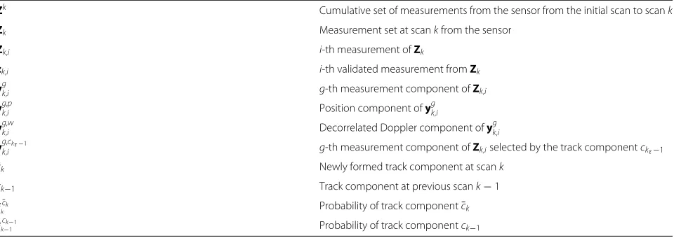
A two-dimensional single-target tracking scenario is pre-sented in Fig. 1. The target can only be detected in the area bounded by the minimum and maximum range and an azimuth between 0 andπ/2. The target is moving with a uniform veloc-ity ofvT =40m/sand with a heading angle of 0◦. The initial

position of the target is described by the polar coordinates

(15, 000 , 1.0472 rad); the maximum possible velocity for the target is assumed to bevmax =400m/s, which is used for the

one-point track initialization. The HPRF radar is stationery in the origin, which returns a set of measurements (which consists of azimuth, range, and Doppler) at each scan; the minimum and maximum of the detection target range areRmax=20km

andRmin=0km, respectively. The radar measurement is

cor-rupted by white Gaussian noise with zero mean and standard deviationσθ =0.1◦,σr=20m, andσd =1m/s, respectively.

(9)

The range measurement is correlated with Doppler measure-ment by coefficientη = −0.8. The radar provides the target position measurement with detection probabilityPd = 0.8.

The uniform clutter position measurement density isρp = 10−7_m−2_{(31 clutter measurements per scan on average). The}

clutter Doppler measurement density is assumed to have a Gaussian probability density function with zero mean and stan-dard deviation of σ_dc = 10m/s. The staggered PRI [22] is applied in the simulations, and the maximum unambiguous range of the HPRF radar isRu(k) =4005m, which results in

five measurement components for each radar returned mea-surement on average. Each simulation experiment consists of 1000 runs, and each run simulates 40 scans with sampling time

T=2m/s.

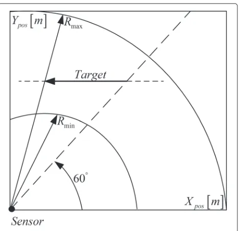
In Fig. 2, a second target is added in the surveillance area crossing the first target, which depicts the multi-target tracking scenario. The second target is moving with a uniform velocity ofvT =46m/sand with a heading angle of 330◦. The initial

position of the second target is(15, 800 , 1.0764 rad). The over-lapping region of both the targets is between scans 17 and 28, where both targets share the measurements dominantly in this region.

The Markov Chain One model [14] of target existence is assumed with transition probabilities

p11=0.98 p12=0.02

p21=0 p22=1 , (70)

where pij denotes the transition probability from event ito

eventj. Event 1 and event 2 representsχkandχ¯k, respectively.

The confirmation thresholds for the algorithms are tuned to deliver the same number of confirmed false tracks (CFT) (≈7) for all 1000 Monte Carlo simulation runs. In both simulation scenarios, the CFT are set to be same for a fair comparison. Both smoothing algorithms consider the lag size of 2.

Fig. 2Simulation scenario for multi-target

The confirmed true track rate for a single target in Fig. 3 presents a comparison between FLs GMM-ITS and other algorithms simulated in this work for single-target tracking. FLs GMM-ITS performs better than both online (GMM-ITS, EMM) algorithms and offline (FLs EMM) tracking algo-rithm under the given surveillance environment.

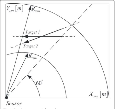
The RMSEs of confirmed true tracks for single-target track-ing scenario are presented in Fig. 4. The smoothtrack-ing algorithms perform better than online algorithms. At the last scank=40, no future information exists, so all algorithms have an identical response in terms of RMSEs.

FLs GMM-ITS and FLs EMM algorithms looks to have sim-ilar RMSEs, although one expects better performance for the FLs GMM-ITS algorithm. The reason is that the true tracks which are confirmed earlier in the FLs GMM-ITS compared to FLs EMM generate less favorable performance in terms of estimation errors.

In Fig. 5, the cumulative confirmed true track rate for the multi-target simulation scenario is presented. From scan 1 to scan 20, the confirmed true track rate reaches to almost 100 %, and the FLs GMM-ITS algorithm shows the fastest response. From scan 20, the online algorithms loose almost 50 % of the targets; in this period, the FLs GMM-ITS algorithm performs better compared to the other algorithms and maintains a high confirmed true track rate. The drop in confirmed true track is expected; when the targets share measurements, the single-target tracking algorithms are expected to loose tracks at a higher rate. The FLs GMM-ITS algorithm recover much faster as compared to other algorithms from scan 28 till the last scan, which indicates the high efficiency of the proposed FLs GMM-ITS algorithm.

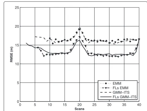
Figures 6 and 7 present the RMSEs for target 1 and tar-get 2, respectively, for the multi-tartar-get simulation scenario depicted in Fig. 2. It is evident that the smoothing algorithms perform significantly better as compared to the online track-ing algorithms. Between scan 17 and scan 28, where the true targets share measurements more prominently, the estimation errors are increased because of association of confirmed true

0 5 10 15 20 25 30 35 40

0 0.1 0.2 0.3 0.4 0.5 0.6 0.7 0.8 0.9 1

Scans

Confirm True Track Rate (%)

EMM FLs EMM GMM−ITS FLs GMM−ITS

(10)

0 5 10 15 20 25 30 35 40 0

5 10 15 20 25

Scans

RMSE (m)

Fig. 4Root mean square error comparison (single target)

track with measurements from other targets. The smoothing algorithms perform much better as compared to the online algorithms and have reduced RMSEs in this interval. The smoothing and filtering algorithms have identical results at the final scan as no future information is available to smooth the target state.

The computational time for the EMM algorithm is set as a reference to determine the percentage of extra computational time needed by other algorithms. The total sampling time is 80, 000 s, which is greater than the computation time of the aforementioned tracking algorithms; therefore, all algorithms are capable of working in real time.

It is evident from the simulation results that use of the smoothing algorithm improves the performance of the tracker in terms of both RMSEs and false track discrimination, at the cost of some delay in both single-target and

multi-0 5 10 15 20 25 30 35 40

0 0.1 0.2 0.3 0.4 0.5 0.6 0.7 0.8 0.9 1

Scans

Confirm True Track Rate (%)

Fig. 5Cumulative confirmed true track rate comparison (multi-target)

0 5 10 15 20 25 30 35 40

0 5 10 15 20 25

Scans

RMSE (m)

Fig. 6Root mean square error comparison (target 1)

target tracking simulation environments. Table 2 provides the comparison of computational time for different tracking algorithms.

8 Conclusions

This paper provides a new procedure to calculate the smoothed target hybrid state at fixed lagN. The benefits of the smooth-ing algorithm are compared for target tracksmooth-ing algorithms in the clutter using the HPRF radar. The smoothed aug-mented states (obtained at each scan in the smoothing inter-val) and their respective weights (calculated using multi-scan target existence events) are used to obtain the fixed lag smoothed trajectory state estimate for the target. The tar-get existence state is also smoothed at fixed lag N using all feasible multi-scan target existence events in the smoothing interval.

0 5 10 15 20 25 30 35 40

0 5 10 15 20 25

Scans

RMSE (m)

(11)

Table 2Computation time [sec]

Algorithm Execution time Percentage

EMM 49,874 Reference

GMM-ITS 50,994 2.3 %

FLs EMM 55,156 10.5 %

FLs GMM-ITS 59,256 12 %

The FLs GMM-ITS performs much better than FLs EMM, GMM-ITS, and EMM algorithms to track the target using an HPRF radar in terms of RMSEs and false track discrimination. The smoothed target hybrid state provides small estimation errors and produces excellent false track discrimination in the simulation conditions used in the proposed work.

Competing interests

The authors declare that they have no competing interests.

Acknowledgments

This work was conducted at High-Speed Vehicle Research Center of KAIST with support of Defense Acquisition Program Administration (DAPA) and Agency for Defense Development (ADD).

Received: 16 February 2015 Accepted: 27 May 2015

References

1. G Morris, L Harkness,Airborne Pulsed Doppler Radar. (Artech House, Norwood, 1996)

2. D Nagel, H Hommel, inProceedings of CIE International Conference on

Radar. A new HPRF mode with highly accurate ranging capability for

future airborne radar (IEEE Beijing, 2001)

3. YZ Guo, ZL Liu, YC Guo, ZL Xu, Multiple models track algorithm for radar with high pulse-repetition frequency in frequency-modulated ranging mode. IET Radar Sonar Navigation.1(1), 1–7 (2007)

4. D Mušicki, TL Song, WC Kim, D Nešiˇc, Non-linear automatic target tracking in clutter using dynamic gaussian mixture. IET Radar Sonar Navig.6(9), 94–100 (2013)

5. YF Shi, TL Song, D Mušicki, Target tracking in clutter using a high pulse repetition frequency radar. IET Radar Sonar Navig.9(3), 1–9 (2014) 6. Y Bar-Shalom, XR Li, T Kirubarajan, Estimation with Applications to Tracking and Navigation: Theory Algorithms and Software (2004) 7. JB Moore, Discrete-time fixed-lag smoothing algorithms. Automatica.

9(2), 163–173 (1973)

8. C Bing, KT Jitendra, Tracking of multiple maneuvering targets in clutter using IMM/JPDA filtering and fixed-lag smoothing. Automatica.37(2), 239–249 (2001)

9. W Koch, Fixed-interval retrodiction approach to Bayesian IMM-MHT for maneuvering multiple targets. IEEE Trans. Aerospace Electronic Sys.36(1), 2–14 (2000)

10. R Chakravorty, S Challa, Augmented state integrated probabilistic data association smoothing for automatic track initiation in clutter. J. Adv. Inf. Fusion.1(1), 63–74 (2006)

11. TL Song, D Mušicki, Smoothing innovations and data association with IPDA. Automatica.48(7), 1324–1329 (2012)

12. D Fraser, J Potter, The optimum linear smoother as a combination of two optimum linear filters. IEEE Trans. Autom. Control.14(4), 387–390 (1969) 13. D Mušicki, TL Song, TH Kim, Smoothing multi scan target tracking in

clutter. IEEE Trans. Signal Process.61(19), 4740–4752 (2013)

14. D Mušicki, R Evans, S Stankovic, Integrated probabilistic data association. IEEE Trans. Autom. Control.39(6), 1237–1241 (1994)

15. D Mušicki, BFL Scala, RJ Evans, Integrated track splitting filter-efficient multi-scan single-target tracking in clutter. IEEE Trans. Aerosp. Electron. Syst.43(4), 1409–1425 (2007)

16. D Mušicki, TL Song, HH Lee, D Nešiˇc, Correlated Doppler-assisted target tracking in clutter. IET Radar Sonar and Navigation.7(1), 937–944 (2012)

17. L Mo, XQ Song, YY Zhou, ZK Sun, Bar-Shalom Y, Unbiased converted measurements for tracking. IEEE Trans. Areosp. Electron. Syst.34(3), 1023–1027 (1998)

18. YF Shi, TL Song, D Mušicki, inInternational Conference on Electronics,

Information and Communications (ICEIC), 2014. Gaussian mixture

measurement model for high pulse-repetition frequency radar tracking in clutter (IEEE Kota Kinabalu, 2014), pp. 1–2

19. Y Bar-Shalom, E Tse, Tracking in a cluttered environment with probabilistic data association. Automatica.11(5), 451–460 (1975) 20. D Mušicki,Automatic tracking of maneuvering targets in clutter using IPDA.

(PhD thesis, University of Newcastle, Australia, 1994)

21. U Khan, D Mušicki, TL Song, inProceedings of 17th International Conference

on Information Fusion (FUSION 2014). A fixed lag smoothing IPDA tracking

in clutter (IEEE Salamanca, 2014)

22. M Skolnic, Introduction to Radar Systems (2003)