State estimation in multi agent decision and control systems

(1)

STATE ESTIMATION IN MULTI-AGENT DECISION

AND CONTROL SYSTEMS

Thesis by

Domitilla Del Vecchio

In Partial Fulfillment of the Requirements for the Degree of

Doctor of Philosophy

California Institute of Technology Pasadena, California

2005

(2)

c

2005 Domitilla Del Vecchio

(3)

(4)

Acknowledgements

(5)

Abstract

This thesis addresses the problem of estimating the state in multi-agent decision and control systems. In particular, a novel approach to state estimation is developed that uses partial order theory in order to overcome some of the severe computational complexity issues arising in multi-agent systems. Within this approach, state estimation algorithms are developed that enjoy provable convergence properties and are scalable with the number of agents.

(6)

List of Figures

2.1 Examples of partial orders . . . 6

2.2 Power lattice . . . 7

2.3 Examples of maps on partial orders . . . 8

2.4 Approximations on a partial order . . . 10

2.5 Weakly equivalent executions . . . 11

2.6 Enumeration approach to state estimation . . . 13

3.1 RoboFlag drill . . . 16

3.2 The RoboFlag Drill . . . 17

3.3 Lower and upper bound description for the RoboFlag drill . . . 18

3.4 Lattice approach to state estimation . . . 20

3.5 Example of estimator convergence plots . . . 21

3.6 RoboFlag drill example . . . 30

3.7 Convergence plots . . . 38

4.1 Transition classes . . . 43

4.2 Automaton example. . . 46

4.3 Automaton example: lattice (χ,≤). . . 46

5.1 Extension ˜f on latticeχ. . . 55

5.2 Estimator convergence plots . . . 59

6.1 Estimator update laws . . . 68

6.2 Hasse diagram representing elements in the lattice (L,≤). . . 72

(10)

6.4 Finite State Machine Example . . . 80

6.6 Monotone system example . . . 83

7.1 Petri net example . . . 93

7.2 Uncertainty on the model (branchings) . . . 110

7.3 Uncertainty on the model (unknown dynamics) . . . 111

(11)

Chapter 1 Introduction

Logic and decision making are playing increasingly large roles in modern control sys-tems, and virtually all modern control systems are implemented using digital computers. Examples include aerospace systems, transportation systems (air, automotive, and rail), communication networks (wired, wireless, and cellular), and supply networks (electrical power and manufacturing). The evolution of these systems is determined by the interplay of continuous dynamics and logic. The continuous variables can represent quantities such as position, velocity, acceleration, voltage, current, etc., while the discrete variables can represent the state of the decision and communication protocol that is used for coordina-tion and control. Most of these systems are also multi-agent, in which an agent can be, for example, a wireless device, a micro-controller, a robot, a piece of machinery, a piece of hardware or software, or even a human. The need for understanding and analyzing the behavior of these systems is compelling. However, the coupling of continuous dynamics and decision protocols renders the system under study interesting and complicated enough that new tools are needed for the sake of analysis and control. Also, multi-agent systems are usually affected by the combinatorial explosion of the state space that renders most of the existing state estimation algorithms inapplicable.

(12)

locationobserver with a Luenberger observer to design hybrid observers that identify the location in a finite number of steps and converge exponentially to the continuous state. However, if the number of locations is large, as in the systems that we consider, such an ap-proach is impracticable. In Balluchi et al., sufficient conditions for a linear hybrid system to be final state determinable are given [5]. In Alessandri et al., Luenberger-like observers are proposed for hybrid systems where the system location is known [2, 3]. Vidal et al. [43] derive sufficient and necessary conditions for observability of discrete time jump-linear systems, based on a simple rank test on the parameters of the model. In later work [44], these notions are generalized to the case of continuous time jump linear systems. For jump Markov linear systems, Costa and do Val derive a test for observability [18], and Cassan-dra et al. propose an approach to optimal control for partially observable Markov decision processes [15]. For continuous time hybrid systems, De Santis et al. propose a definition of observability based on the possibility of reconstructing the system state, and testable conditions for observability are provided [28].

In the discrete event literature, observability has been defined by Ramadge [38], for example, who derives a test for current state observability. Oishi et al. [37] derive a test for immediate observability in which the state of the system can be unambiguously recon-structed from the output associated with the current state and last and next events. ¨Ozveren et al. [22] and Caines [13, 14] propose discrete event observers based on the construction of the current-location observation tree that is impracticable when the number of locations is large, which is our case. Observability is also considered in the context of distributed monitoring and control in industrial automation, where agents are cooperating to perform system-level tasks such as failure detection and identification on the basis of local informa-tion [39]. Diaz et al. consider observers for formal on-line validainforma-tion of distributed systems, in which the on-line behavior is checked against a formal model [29]. In the context of sen-sor networks, state estimation covers a fundamental role when solving surveillance and monitoring tasks in which the state usually has several components, such as the position of an agent, its identity, and its intent (see for example [17] or [11]).

(13)

These complexity issues render prohibitive the estimation problem for systems with a large discrete state space, which is often the case in multi-agent systems. Our point of view is that some of the complexity issues, such as those encountered in [13] or [4], can be avoided by finding a good way of representing the sets of interest and by finding a good way of computing maps on them. As a naive example, consider the set S of all natural numbers between one and one thousand. This set is usually represented as an interval in

N, that is_S = [1,1000], so that the listing of all the elements it contains is not necessary

for representing it. Suppose we want to know what the setSis mapped to by a mapφthat

associates each elementnwith the elementn+2. Clearly, to computeφ(S) we do not need to computeφon each element ofSand collect all the results. In fact, it is easy to see that

φ(S) = [3,1002], that is, we just compute φon the least and maximum elements of Sto obtain the least and maximum elements ofφ(S), which are then used to represent the latter set. This simplification is possible thanks to the order structure naturally associated withN

and thanks to the structure of the mapφ.

These ideas are extended by using partial order theory to an arbitrary set, which might be more complicated than a set in N and might contain continuous components. Partial

order theory has been used historically in theoretical computer science to prove properties about convergence of algorithms [19]. It has also been used for studying controllability properties of finite state machines [12] and for approaching the state explosion problem in the verification of concurrent systems [31]. In this work, we exploit partial order theory to estimate the state in systems with a large discrete space. In particular, given a systemΣ defined on its space of variables, we extend it to a larger space of variables that has lattice structure so as to obtain an extended system ˜Σ. Under certain properties verified by the extension ˜Σ, an observer for systemΣcan be constructed, which updates at each step only two variables. It updates the least and greatest element of the set of all values of variables compatible with the output sequence and with the dynamics of Σ. The structure of the obtained observer resembles the structure of the Luenberger observer or a Kalman filter as it is obtained by “copying” the dynamics of the systemΣand by correcting it according to the measured output values.

(14)

state is measured, and with the estimation of the whole system state in case a cascade structure of the estimator is possible. Within this context, the proposed estimation approach is also general as it applies to any observable system. In fact, we show that a system is observable if and only if there is a lattice in which the extended system satisfies the requirements for the construction of the proposed estimator. Within the state estimation framework that we develop, the estimation of the discrete and continuous part of the state space is handled in a unified way. In fact, there is no need to implement both a continuous state estimator that relies on classical control theory and a discrete state estimator based on automata theory, as done in most previous work. This is achieved by using a partial order to establish relationships between elements of a discrete space in analogy to how a metric establishes relationships between elements in a continuous space.

(15)

Chapter 2 Basic Concepts

In this chapter, we review some basic notions that will be used throughout this work. First, we give some background on partial order and lattice theory in Section 2.1 (for more details the reader is referred to [21, 1]). The theory of partial orders, while standard in computer science, may be less well known to the intended audience of this thesis. Then, the class of systems under study is introduced in Section 2.2, i.e., deterministic transition systems, and the state estimation problem is defined. Finally, we show a solution to the problem in Section 2.3, an enumeration method that has been most often used in previous work.

2.1 Partial Order Theory

A partial order is a setχwith a partial order relation “≤”, and we denote it by the pair (χ,≤). For any x,w ∈ χ, sup{x,w}is the smallest element that is larger than both xand

w. In a similar way, inf{x,w}is the largest element that is smaller than both xandw. We define thejoin“g” and themeet“f” of two elementsxandwinχas

1. xgw:=sup{x,w}andxfw:= inf{x,w};

2. ifS ⊆χ,WS :

=sup S, andVS :

=inf S.

Let (χ,≤) be a partial order. If x_fw ∈ χand xgw ∈ χfor any x,w ∈ χ, then (χ,≤)

(16)

From the diagrams, it is easy to tell when one element is less than another: x < wif and

only if there is a sequence of connected line segments moving upward from xtow.

xgw

x w

xfw

w xfw

xfw

xgw

x

a) b)

d) c)

[image:16.612.251.403.124.298.2]

w x

Figure 2.1: In diagram a) and b), xandware not related, but they have a join and a meet, respectively. In diagram c), we show a complete lattice. In diagram d), we show a partially ordered set that is not a lattice, since the elements xandwhave a meet, but not a join.

Let (χ,≤) be a partial order. Then (χ,≤) is a chainif for all x,w ∈ χ, either x ≤ w or w ≤ x, that is, any two elements are comparable. If instead any two elements are not comparable, i.e., x≤ yif and only ifx = y, (χ,≤) is said to be ananti-chain. If x < wand

there is no other element in betweenxandw, we writex w.

Let (χ,≤) be a lattice and let S ⊆ χ be a non-empty subset of χ. Then, (S,≤) is a

sublattice ofχ if a,b ∈ S implies that a_g b ∈ S and a_f b ∈ S. If any sublattice of χ

contains its least and greatest elements, then (χ,≤) is calledcomplete. Any finite lattice is complete, but infinite lattices may not be complete, and hence the significance of the notion of a complete partial order [1]. Given a complete lattice (χ,≤), we will be concerned with a special kind of a sublattice called aninterval sublatticedefined as follows. Any interval sublattice of (χ,≤) is given by [L,U] = {w ∈ χ : L ≤ w ≤ U} for L,U ∈ χ. That is,

this special sublattice can be represented by two elements only. For example, the interval sublattices of (R_,_≤) are just the familiar closed intervals on the real line. A particular

instance of a partial order is thef-semilattice, which is a partially ordered set in which all

(17)

Let (χ,≤) be a lattice with least element⊥(the bottom). Then,a∈χis called anatom

of (χ,≤) ifa>⊥and there is no elementbsuch that⊥<b <a. The set of atoms of (χ,≤) is denotedA(χ,≤).

Thepower latticeof a setU, denoted (P(U),⊆), is given by the power set ofU,P(U) (the set of all subsets ofU), ordered according to the set inclusion⊆. The meet and join of the power lattice is given by intersection and union. The bottom element is the empty set, that is,⊥= ∅, and the top element isU itself, that is,>=U. Note thatA(P(U),⊆)=U. An example is illustrated in Figure 2.2. Given a setP, we denote by|P|its cardinality.

α₁ _α₂

α₃

U={α₁, α₂, α₃} >=α₁_gα₂_gα₃=U

α₁_gα₂={α₁, α₂}

α₁_gα₃={α₁, α₃}

α₂_gα₃={α₂, α₃}

(χ,≤)=(P(U),⊆)

[image:17.612.253.432.253.419.2]

⊥=∅

Figure 2.2: Power lattice (χ,≤) of a setUcomposed of three elements.

Definition 2.1.1. Let (P,≤) and (Q,≤) be partially ordered sets. A map f :P→Qis (i) anorder preserving mapifx≤w =⇒ f(x)≤ f(w);

(ii) anorder embeddingifx≤ w⇐⇒ f(x)≤ f(w);

(iii) anorder isomorphismif it is order embedding and it mapsP onto Q.

Definition 2.1.2. If (P,≤) and (Q,≤) are lattices, then a map f : P → Q is said to be a

homomorphismif f isjoin-preservingandmeet-preserving, that is, for allx,w∈Pwe have that f(xgw)= f(x)g f(w) and f(xfw)= f(x)f f(w).

Proposition 2.1.1. (See [21]) If f : P → Q is a bijective homomorphism, then it is an

(18)

z

x w

y

z

x w

y

f

e)

f(z)= f(w)

f(x)= f(y)

f(z)

f(x)

f(y)

[image:18.612.226.447.52.274.2]

f(w) f)

Figure 2.3: In diagram e), we show a map that is, order preserving but not order embedding. In diagram f), we show an order embedding that is, not an order isomorphism: any two elements maintain the same order relation, but in between zandwthere is nothing, while in between f(z) and f(w) some other elements appear (it is not onto).

Every order isomorphic map faithfully mirrors the structure ofPontoQ. In Figure 2.3 we show some examples.

The notion of an order preserving map can be generalized to the case in which the map is nondeterministic, that is, it maps an element to a set of possible elements. With a slight abuse of the term “order preserving” we also make the following non-standard definition. Definition 2.1.3. Let x,w∈χ, with (χ,≤) a lattice,x≤ w, and f : χ→ P(χ). We say that

f isorder preservingifWf(x)_≤ Wf(w) andVf(x)_≤ Vf(w).

A partial order induces a notion of distance between elements in the space. Define the distance function on a partial order in the following way.

Definition 2.1.4. (Distance on a partial order) Let (P,≤) be a partial order. A distancedon (P,≤) is a functiond:P×P→Rsuch that the following properties are verified:

(i) d(x,y)≥0 for any x, y∈Pandd(x,y)= 0 if and only ifx=y; (ii) d(x,y)=d(y,x);

(19)

Since Chapter 6 deals with a partial order on the space of the discrete variables and with a partial order on the space of the continuous variables, it is useful to introduce the Cartesian product of two partial orders as it can be found in [1].

Definition 2.1.5. (Cartesian product of partial orders) Let (P1,≤) and (P2,≤) be two partial

orders. Their Cartesian product is given by (P1 × P2,≤), where P1 × P2 = {(x,y) | x ∈

P1 and y ∈ P2}, and (x,y) ≤ (x0,y0) if and only if x ≤ x0 and y ≤ y0. For any (p1,p2) ∈

P1 ×P2 the standard projectionsπ1 : P1× P2 → P1 andπ2 : P1×P2 → P2 are such that

π1(p1,p2)= p1 andπ2(p1,p2)= p2.

One can easily verify that the projection operators preserve the orders.

In this work we will also deal with approximations of sets and elements of a partial order. We thus give the following definition.

Definition 2.1.6. (Upper and lower approximation) LetP1andP2be two sets withP1⊆ P2

and (P2,≤) a partial order. For any x∈P2, we define thelower and upper approximations

ofxinP1as

aL(x) :=max

(P2,≤){w∈P1 |w≤ x}

aU(x) := min

(P2,≤){w∈P1 |w≥ x}.

If such lower and upper approximations exist for any x ∈P2, then the partial order (P2,≤)

is said to beclosed with respect to P1.

One can verify that the lower and upper approximation functions are order preserving. This means that for anyx1,x2 ∈P2withx1 ≤ x2, thenaL(x1)≤aL(x2) andaU(x1)≤ aU(x2).

Example of lower and upper approximations are depicted in Figure 2.4.

(20)

aL(x)

x

inP1

inP2 and not inP1

[image:20.612.218.399.64.208.2]

aU(x)

Figure 2.4: LetP1 ⊆ P2, the open circles represent elements inP2that are not inP1while

the filled circles represent elements that are also inP1.

2.2 Deterministic Transition Systems

The class of systems we are concerned with are deterministic, infinite state systems with output. The following definition introduces such a class.

Definition 2.2.1.(Deterministic transition systems) Adeterministic transition system(DTS) is the tupleΣ =(S,Y,F,g), where

(i) S is a set of states withs∈S; (ii) Yis a set of outputs withy∈ Y;

(iii) F :S →S is the state transition function; (iv) g:S → Yis the output function.

An execution of Σ is any sequence σ = {s(k)}_k∈N such that s(0) ∈ S and s(k+ 1) =

F(s(k)) for all k ∈ N. The set of all executions ofΣis denotedE(Σ). An output sequence ofΣis denotedy={y(k)}_k∈N, withy(k)=g(σ(k)), forσ∈ E(Σ).

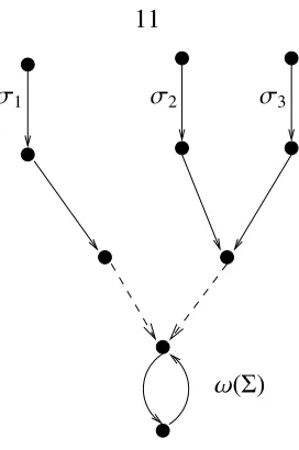
Definition 2.2.2. LetΣ = (S,Y,F,g) be a deterministic transition system. The setΩ ⊂ S is the ω+_{-limit set} _of _Σ_{, denoted} _ω₍_Σ_{), if it is the smallest subset of} _S _{such that for all}

σ={s(k)}k∈N

(21)

σ1 σ2 σ3

[image:21.612.257.393.50.255.2]

ω(Σ)

Figure 2.5: Executionsσ2andσ3are weakly equivalent according to Definition 2.2.5 while

σ1is not weakly equivalent to eitherσ2orσ3.

(ii) for eachσ ∈ E(Σ), there existsk_σ such thatσ(kσ)∈Ω.

Definition 2.2.3. Given a deterministic transition systemΣ = (S,Y,F,g), two executions σ1, σ2∈ E(Σ) aredistinguishableif there exists aksuch thatg(σ1(k)),g(σ2(k)).

Definition 2.2.4. (Observability) The deterministic transition system Σ = (S,Y,F,g) is

said to beobservableif any two different executionsσ1, σ2∈ E(Σ) are distinguishable.

From this definition, we deduce that if a systemΣis observable, any two different initial states will give rise to two executionsσ1andσ2with different output sequences. Thus, the

initial states can be distinguished by looking at the output sequence. However, there are systems for which two different initial states cannot be distinguished, but the states at some later step can. We introduce a weaker notion of observability analogous to detectability

[41] that accounts for this distinction.

Definition 2.2.5. Given a deterministic transition systemΣ = (S,Y,F,g), two executions σ1, σ2∈ E(Σ) areweakly equivalent, denotedσ1 ∼σ2, if there existsk∗such thatσ1(k∗)<

ω(Σ) andσ1(k)=σ2(k) for allk≥k∗.

In Figure 2.5, we show examples of equivalent and not equivalent system executions. Definition 2.2.6. (Weak observability) A deterministic transition systemΣ =(S,Y,F,g) is

(22)

For any systemΣ, the state estimation problem is defined as follows.

Problem 2.2.1. (State estimation problem) GivenΣand any output sequencey= {y(k)}_k∈N,

determine{s(k)}k≥k0 for somek0 > 0.

In the next section, a solution to this problem, first introduced by Caines ([13, 14]), is presented.

2.3 Enumeration Approach to the Discrete State

Estima-tion Problem

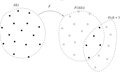
Let Σ = (S,Y,F,g), withS a finite set and Y = {Y1, ...,Ym} with m ≤ |S|. We use a variable ˆsto represent an estimate of swith ˆs ∈ P(S). Since S is composed by a finite number of elements, the estimation problem is called the discrete state estimation problem. The intention is that ˆs(k) denotes the set of all possible values of s(k) compatible with the output sequence until step k and with the system dynamics. For k ≥ 0, ˆs(k) is updated according to

ˆ

s(k+1)= F(ˆs(k))∩Oy(k+1), sˆ(0)=S, (2.1)

where for any ˆs∈ P(S), we define

F(ˆs)= {s0 ∈S : ∃ s∈sˆwithF(s)= s0},

and Oy is the output set and it is defined by Oy := g−1(y), with g−1 : Y → P(S) is the inverse ofgdefined as

g−1₍_y₎₌_{_s_∈_S _: _g₍_s₎₌_y_}_.

Equation (2.1) gives at each step k a set that contains all and only the states compat-ible with the system dynamics and with the output sequence up to stepk+ 1. A picture representing this update law is in Figure 2.6.

(23)

F

ˆ

s(k)

F(ˆs(k))

[image:23.612.112.521.62.312.2]

Oy(k+1)

Figure 2.6: Enumeration approach to state estimation: the set of possible consistent states ˆ

s(k) is mapped forward through the system dynamics F, and then F(ˆs(k)) is intersected with the set of all states compatible with the new output (Oy(k+1)). This procedure gives

ˆ

s(k+1), which is represented by the filled circles in the right diagram.

Theorem 2.3.1. Given the systemΣ =(S,Y,F,g), the update law in equation (2.1) is such

that

(i) s(k)∈sˆ(k)for any k ≥0(correctness);

(ii) |sˆ(k+1)| ≤ |sˆ(k)|(non-increasing error);

(iii) ifΣis (weakly) observable, then there is k₀ > 0such thatsˆ(k) = s(k)for any k ≥ k₀

(convergence).

Proof. Proof of (i). This can be proved by induction argument on the step k. Briefly,

s(0) ∈ sˆ(0). Assume s(k) ∈ sˆ(k), we prove that s(k+1) ∈ sˆ(k+ 1). This follows from two facts. Fact 1): s(k+1) ∈g−1₍_y₍_k₊_{1)) because}_g₍_s₍_k₊₁₎₎ ₌ _y₍_k₊_{1). Fact 2): Since}

s(k)∈ sˆ(k), alsos(k+1)= F(s(k))∈F(ˆs(k)).

(24)

Proof of (iii). This can be proved by contradiction. Assume that there is no k0 such

that ˆs(k)= s(k), then one can construct two executions ofΣ,σ1 ,σ2 such thatg(σ1(k)) =

g(σ2(k)) for anyk. This contradicts (weak) observability.

This proof is just a sketch. For a complete proof, the reader is deferred to [13]. This enumeration approach to state estimation will also be referred to as current location obser-vation tree method, due to the tree implementation provided in [13].

(25)

Chapter 3 Construction of Discrete State

Estimators on a Lattice

In the previous chapter, we have shown an enumeration approach to the discrete state estimation problem (first introduced by Caines [13]). Such an approach is however imprac-ticable when the dimension of the state space is large as is often the case in multi-agent or distributed systems. In this chapter, we propose an alternative to the enumeration of the compatible states. In particular, a set is represented by a lower and an upper bound once it has been immersed in a lattice structure. We then keep track of the set by updating its lower and upper bounds as opposed to the list of elements it contains. As a motivating example, we introduce in Section 3.1 a multi-robot system. In Section 3.2, the state estima-tion problem is formulated on a lattice, and a soluestima-tion is proposed in Secestima-tion 3.3. Finally, the example presented in Section 3.1 is revisited, and the estimator constructed in Section 3.4. The results of this chapter appeared in [23].

3.1 Motivating Example

As a motivating example, we consider a task that represents a defensive maneuver for a robotic “capture the flag” game [20]. We do not propose to devise a strategy that addresses the full complexity of the game. Instead, we examine the following very simple drillor exercise that we call “RoboFlag Drill.” Some number of blue robots with positions (zi,0)∈

R2 (denoted by open circles) must defend their zone _{(x_,y) _∈ R2 _| y _≤ 0_} from an equal

(26)

are (xi,yi)∈R2. An example for 5 robots is illustrated in Figure 3.1.

z2

z1 z3 z4 z5

(x1,y1)

(x2,y2)

(x3,y3)

(x5,y5)

[image:26.612.251.389.100.314.2]

(x4,y4)

Figure 3.1: An example state of the RoboFlag Drill for 5 robots. The dashed lines represent the assignment of each blue robot to red robot. Here, the assignment isα = {3,1,5,4,2}. The variableszi denotes the position along the horizontal axis of blue roboti, and (xi,yi) denotes the position in the plane of red roboti.

The red robots move straight toward the blue robots’ defensive zone. The blue robots are each assigned to a red robot, and they coordinate to intercept the red robots. Let N

represent the number of robots in each team. The robots start with an arbitrary (bijective) assignmentα:{1, ...,N} → {1, ...,N}, whereαiis the red robot that blue robotiis required to intercept. At each step, each blue robot communicates with its neighbors and decides to either switch assignments with its left or right neighbor or keep its assignment. It is possible to show that theαassignment reaches the equilibrium value (1, ...,N) (see [35] or

[34] for details). We consider the problem of estimating the current assignmentαgiven the

(27)

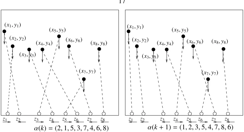
(x3,y3) (x4,y4)

(x5,y5) (x6,y6)

(x7,y7) (x8,y8)

α(k)= (2,1,5,3,7,4,6,8)

z1 z2 z3 z4 z5 z6 z7 z8 (x1,y1)

(x2,y2)

(x3,y3) (x4,y4)

(x5,y5) (x6,y6)

(x7,y7) (x8,y8)

(x1,y1)

(x2,y2)

α(k+1)= (1,2,3,5,4,7,8,6)

[image:27.612.118.530.57.281.2]

z1 z2 z3 z4 z5 z6 z7 z8

Figure 3.2: Example of the RoboFlag Drill with 8 robots per team. The dashed lines represent the assignment of each blue robot to red robot. The arrows denote the direction of motion of each robot.

The RoboFlag Drill system can be specified by the following rules:

yi(k+1)= yi(k)−δ if yi(k)≥δ (3.1)

zi(k+1)= zi(k)+δ if zi(k)< xαi(k) (3.2)

zi(k+1)= zi(k)−δ if zi(k)> xαi(k) (3.3)

(αi(k+1), αi+1(k+1))= (αi+1(k), αi(k)) if xαi(k) ≥zi+1(k)∧xαi+1(k)≤ zi+1(k), (3.4)

where we assumezi ≤ zi+1and xi < zi < xi+1 for allk. Also, if none of the “if” statements

(28)

Equation (3.4) establishes that two robots trade their assignments if the current assign-ments cause them to go toward each other. The question we are interested in is the follow-ing: given the evolution of the measurable quantitiesz, x,y, can we build an estimator that tracks on-line the value of the assignmentα(k)? The value ofα∈perm(N) determines the discrete state, i.e.,S = perm(N). The discrete stateαdetermines also what has been called

in previous work the location of the system (see [4]). The number of possible locations is N!, that is, |S| = N!. This for N ≥ 8 renders prohibitive the application of location observers based on the current location observation tree as described in [13] (revised in Chapter 2) and used in [4], [22]. At each step, the set of possibleαvalues compatible with

the current output and with the previously seen outputs can be so large as to render imprac-tical its computation. As an example, we consider the situation depicted in Figure 3.2 (left)

stepk zmotion at observation of [                                    2 1 4 1 6 1 1 1                                    ,                                    8 2 8 4 8 6 7 8                                    ]

Oy(k)

˜ f [                                    1 2 1 4 1 6 1 1                                    ,                                    2 8 4 8 6 8 7 8                                    ] ˜

f(Oy(k))

[                                    1 1 1 5 1 7 1 1                                    ,                                    1 2 3 8 5 8 7 8                                    ]

Oy(k+1)

[image:28.612.119.515.333.475.2]

∩ =[                                    1 2 1 5 1 7 1 1                                    ,                                    1 2 3 8 5 8 7 8                                    ]

Figure 3.3: The observation of thezmotion at stepkgives the set of possibleα,Oy(k). At

each step, the set is described by the lower and upper bounds of aninterval sublatticein an appropriately defined lattice. Such set is then mapped through the system dynamics ( ˜f) to obtain at stepk+1 the set ofαthat are compatible also with the observation at stepk. Such

a set is then intersected withOy(k+1), which is the set ofαcompatible with thezmotion

observed at stepk+1.

where N = 8. We see the blue robots 1,3,5 going right and the others going left. From

equations (3.2)–(3.3) withxi < zi < xi+1we deduce that the set of all possibleα∈perm(N)

compatible with this observation is such that αi ≥ i+ 1 for i ∈ {1,2,3} and αi ≤ i for

(29)

Such a set is then intersected with the set ofαvalues compatible with the new observation.

To overcome the complexity issue that comes from the need of listing 40320 elements for performing such operations, we propose to represent a set by a lower L and an upper U

elements according to some partial order. Then, we can perform the previously described operations only onLandU, two elements instead of 40320. This idea is developed in the following paragraph.

For this example, we can viewα∈NN. The set of possible assignments compatible with

the observation of thezmotion deduced from the equations (3.2)–(3.3), denotedOy(k), can be represented as an interval with the order established component-wise, see the diagram in Figure 3.3. The function ˜f that maps such a set forward, specified by the equations (3.4) with the assumption that xi <zi < xi+1, simply swaps two adjacent robot assignments

if these cause the two robots to move toward each other. Thus, it maps the set Oy(k) to the set ˜f(Oy(k)) shown in Figure 3.3, which can still be represented as an interval. When the new output measurement becomes available (Figure 3.2, right) we obtain the new set

Oy(k+ 1) reported in Figure 3.3. The sets ˜f(Oy(k)) and Oy(k+ 1) can be intersected by simply computing the supremum of their lower bounds and the infimum of their upper bounds. This idea is also explained in Figure 3.4. This way, we obtain the system that updates Land U, beingL and U the lower and upper bounds of the set of all possibleα

compatible with the output sequence:

L(k+1) = f˜(sup(L(k),infOy(k)))

U(k+1) = f˜(inf(U(k),supOy(k))). (3.5)

The variables L(k) and U(k) represent the lower and upper bound, respectively, of the set ˆ

scomputed in equation (2.1). The computational burden of this implementation is of the order of N if N is the number of robots. This computational burden is to be compared to

N!, which is the computation requirement that we have with the enumeration approach as noticed earlier in this section.

(30)

U(k)

L(k)

˜

f(U(k)) ˜

f

supOy(k+1)

infOy(k+1) ˜

f(L(k))

inf( ˜f(U(k)),supOy(k+1))

[image:30.612.145.536.51.337.2]

sup( ˜f(L(k)),infOy(k+1))

Figure 3.4: Lattice approach to state estimation. The set of possible consistent states ˆs(k) is represented by a lower and an upper bound L(k) and U(k), once the set has been im-mersed into a lattice. Then, the function ˜f is computed on L(k) and U(k), only. The intersection with the output set at stepk,Oy(k+1) =[infOy(k+1),supOy(k+1)], is com-puted by computing the supremum and infimum of the set intersection. Its supremum is inf( ˜f(U(k)),supOy(k+1)) and its infimum is sup( ˜f(L(k)),infOy(k+1)).

|[L(k),U(k)]∩perm(N)|, Figure 3.5 shows convergence plotsV(k) for the estimator com-pared to the convergence plotsE(k) =1/NPN

i=1|αi(k)−i|of the assignment protocol to its

equilibrium (1, ...,N).

This example gives an idea of how complexity issues can be overcome with the aid of some partial order structure. In particular, the function ˜f has the property of preserving the interval structure of the sets of interest: this is a key property that allows to use of upper lower bounds only for computation purposes. In a more general setting, one would like to know what are the system properties that allow such simplifications. By using partial order theory, we address this question.

(31)

esti-1 2 3 4 5 6 7 8 9 10 0

10 20

1 2 3 4 5 6 7 8 9 10

0 5 10 15

1 2 3 4 5 6 7 8 9 10

0 10 20

time

[image:31.612.211.436.70.270.2]

dashed line = E(k) solid line = log of V(k) N=8: results for different initial conditions

Figure 3.5: Convergence plots for the estimator (V(k)) compared to the convergence plot of the assignment protocol to its equilibrium (E(k)).

mation problem is then stated as the problem of finding suitable update laws for the upper and lower bounds of the set of all possible discrete variable values compatible with the output sequence. A solution to this problem is proposed in Theorem 3.3.1.

3.2 Problem Formulation

The deterministic transition systems Σ we defined in the previous chapter are quite general. In this section, we restrict our attention to systems with a specific structure. In particular, for a systemΣ =(S,Y,F,g) we suppose that

(i) S =U × ZwithU a finite set andZa finite dimensional space; (ii) F = (f,h), where f :U × Z → Uandh:U × Z → Z;

(iii) y=g(α,z) := z, whereα∈ U, z∈ Z,y∈ Y, andY= Z.

The set U is a set of logic states and Z is a set of measured states or physical states, as one might find in a robot system. In the case of the example given in Section 3.1, U = perm(N) and Z = RN, the function f is represented by equations (3.4) and the

(32)

of deterministic transition systems by Σ = S(U,Z, f,h) where we associate to the tuple

(U,Z, f,h), the equations:

α(k+1) = f(α(k),z(k))

z(k+1) = h(α(k),z(k)) (3.6)

y(k) = z(k),

whereα ∈ U andz ∈ Z. An execution of the systemΣ in equations (3.6) is a sequence

σ = {α(k),z(k)}_k∈N. The output sequence is {y(k)}k∈N = {z(k)}k∈N. Given an execution σ

of the system Σ, we denote the αandzsequences corresponding to such an execution by

{σ(k)(α)}k∈Nand{σ(k)(z)}k_∈N, respectively.

From the measurement of the output sequence, which in our case coincides with the evolution of the continuous variables, we want to construct a discrete state estimator: a system ˆΣ that takes as input the values of the measurable variables and asymptotically tracks the value of the variableα. We thus define in the following definition a deterministic

transition system with input.

Definition 3.2.1. (Deterministic transition system with input) A deterministic transition system with input is a tuple (S,I,Y,F,g) in which

(i) S is a set of states; (ii) Iis a set of inputs; (iii) Yis a set of outputs;

(iv) F :S × I →S is a transition function; (v) g:S → Yis an output function.

In Problem 3.2.1 below, we specify what the elements of this tuple are when the DTS with input is a discrete state estimator of a DTSΣ = S(U,Z, f,h). First, note that the set

(33)

the observation and with the system dynamics given in (3.6). This enumeration approach has been shown in Section 2.3, in which the estimate is a list of possible values that the estimator has to update when a new measurement becomes available. This method leads to computational issues when the set to be listed is large.

In this chapter, an alternative to simply maintaining a list of all possible values forαis

proposed. We find a representation of the set so that the estimator updates the representation of the set rather than the whole set itself. In particular, if the set U can be immersed in a larger setχ whose elements can be related by an order relation≤, we could represent a subset of (χ,≤) as an interval sublattice [L,U]. Let “id” denote the identity operator. We

formulate the discrete state estimation problem on a lattice as follows.

Problem 3.2.1. (Discrete state estimator on a lattice) Given the deterministic transition systemΣ =S(U,Z, f,h), find a deterministic transition system with input ˆΣ =(χ×χ,Z × Z, χ×χ,(f1, f2),id), with f1 :χ× Z × Z →χ, f2:χ× Z × Z →χ,U ⊆χ, with (χ,≤) a

lattice, represented by the equations

L(k+1) = f₁(L(k),y(k),y(k+1))

U(k+1) = f₂(U(k),y(k),y(k+1)),

withL(k)∈χ,U(k)∈χ, L(0) :=V

χ,U(0) := W

χ, such that

(i) L(k) ≤α(k)≤U(k) (correctness);

(ii) |[L(k+1),U(k+1)]| ≤ |[L(k),U(k)]|(non-increasing error);

(iii) There exists k0 > 0 such that for any k ≥ k0 we have [L(k),U(k)] ∩ U = α(k)

(convergence).

3.3 Problem Solution

For finding a solution to Problem 3.2.1, we need to find the functions f1and f2defined

(34)

definitions a way of extending a system Σ defined onU to a system ˜Σ defined on χwith

U ⊆ χ. Moreover, as we have seen in the motivating example, we want to represent the

set of possibleα values compatible with an output measurement as an interval sublattice

in (χ,≤). We thus define the ˜Σ transition classes, with each transition class corresponding to a set of values inχcompatible with an output measurement. We define the partial order

(χ,≤) and the system ˜Σ to be interval compatible if such equivalence classes are interval sublattices and ˜Σ preserves their structure. On the basis of such notions, Theorem 3.3.1 below gives a possible solution to Problem 3.2.1.

Definition 3.3.1.(Extended system) Given the deterministic transition systemΣ =S(U,Z,

f,h), an extension of Σ on χ, with U ⊆ χ and (χ,≤) a finite lattice, is any system ˜Σ = S(χ,Z, f˜,h˜), such that

(i) ˜f :χ× Z →χand ˜f|U×Z = f;

(ii) ˜h:χ× Z → Zand ˜h|U×Z =h.

Definition 3.3.2. (Transition sets) Let ˜Σ = S(χ,Z, f˜,h˜) be a deterministic transition

sys-tem. The non empty setsT(z1_,_z2₎( ˜Σ) = {w∈ χ| z2 = h˜(w,z1)}, forz1,z2 ∈ Z, are named the ˜

Σ-transition sets.

Each ˜Σ-transition set contains all ofw∈χvalues that allow the transition fromz1 toz2

through ˜h. It will be also useful to define the transition classTi( ˜Σ), which corresponds to multiple transition sets, as transition sets obtained by different pairs (z1,z2) can define the

same set inχ.

Definition 3.3.3. (Transition classes) The setT( ˜Σ) = {T₁( ˜Σ), ...,TM( ˜Σ)}, withTi( ˜Σ) such that

(35)

Note that T(z1_,_z2₎ and T₍_z3_,_z4₎ might be the same set even if (z1,z2) , (z3,z4): in the

RoboFlag Drill example introduced in Section 3.1, if robot j is moving right, the set of possible values ofαj is [j+1,N] independently of the values ofzj(k). Thus, T(z1_,_z2₎ and

T(z3_,_z4₎can define the same set that we callTi( ˜Σ) for somei. Also, the transition classesTi( ˜Σ) are not necessarily equivalence classes as they might not be pairwise disjoint. However, for the RoboFlag Drill it is the case that the transition classes are pairwise disjoint, and thus they partition the lattice (χ,≤) in equivalence classes.

Definition 3.3.4. (Output set) Given the extension ˜Σ = S(χ,Z, f˜,h˜) of the deterministic

transition system Σ = S(U,Z, f,h) on the lattice (χ,≤), and given an output sequence {y(k)}_k∈NofΣ, the set

Oy(k) :={w∈χ|h˜(w,y(k)) =y(k+1)}

is theoutput setat stepk.

Note that by definition, for anyk, Oy(k) = T₍_y₍_k₎_,_y₍_k₊₁₎₎( ˜Σ), and thus it is equal toTi( ˜Σ) for somei ∈ {1, ...,M}. The output set at step kis the set of all possiblewvalues that are compatible with the pair (y(k),y(k+1)). By definition of the extended functions (˜h|U×Z =

h), this output set contains also all of the values ofαcompatible with the same output pair.

Definition 3.3.5. (Interval compatibility) Given the extension ˜Σ = S(χ,Z, f˜,h˜) of the

system Σ = S(U,Z, f,h) on the lattice (χ,≤), the pair ( ˜Σ,(χ,≤)) is said to be interval

compatibleif

(i) each ˜Σ-transition class,Ti( ˜Σ)∈ T( ˜Σ), is an interval sublattice of (χ,≤):

Ti( ˜Σ)=[^

Ti( ˜Σ),_

Ti( ˜Σ)];

(ii) ˜f : (Ti( ˜Σ),z) → [ ˜f(V_Ti( ˜_Σ)

,z), f˜(W_Ti( ˜_Σ)

,z)] is an order isomorphism for any i ∈ {1, ...,M}and for anyz∈ Z.

(36)

Theorem 3.3.1. Assume that the deterministic transition systemΣ = S(U,Z, f,h)is

ob-servable. If there is a lattice(χ,≤), such that the pair( ˜Σ,(χ,≤))is interval compatible, then

the deterministic transition system with inputΣ =ˆ (χ×χ,Z × Z, χ×χ,(f1, f2),id)with

f1(L(k),y(k),y(k+1)) = f˜

L(k)g^Oy(k),y(k)

f2(U(k),y(k),y(k+1)) = f˜

U(k)f_Oy(k),y(k)

solves Problem 3.2.1.

Proof. In order to prove the statement of the theorem, we need to prove that the system

L(k+1) = f˜(L(k)_g^

Oy(k),y(k))

U(k+1) = f˜(U(k)_f_

Oy(k),y(k)) (3.7)

withL(0)=V

χ,U(0)= W

χis such that properties (i)–(iii) of Problem 3.2.1 are satisfied.

For simplicity of notation, we omit the dependence of ˜f on its second argument.

Proof of (i): This is proved by induction on k. Base case: for k = 0 we have that

L(0) = V

χand thatU(0) = W

χ, so thatL(0) ≤ α(0) ≤ U(0). Induction step: we assume that L(k) ≤ α(k) ≤ U(k) and we show that L(k+ 1) ≤ α(k +1) ≤ U(k +1). Note that

α(k)∈Oy(k). This, along with the assumption of the induction step, implies that

L(k)g^Oy(k)≤ α(k)≤ U(k)f_Oy(k).

This last relation also implies that there isxsuch thatx≥ L(k)_gVOy(k) andx_≤ W Oy(k).

This in turn implies that

L(k)g^Oy(k)≤_Oy(k).

This in turn implies that L(k)gVOy(k) ∈ Oy(k). Because of this, because (by analogous

reasonings)U(k)fWOy(k)∈Oy(k), and because the pair ( ˜Σ,(χ,≤)) is interval compatible,

we can use the isomorphic property of ˜f (property (ii) of Definition 3.3.5), which leads to

˜

(37)

This relationship combined with equation (3.7) proves (i).

Proof of (ii): This can be shown by proving that for anyw∈[L(k+1),U(k+1)] there isz ∈[L(k),U(k)] such thatw = f˜(z). By equation (3.7),w∈ [L(k+1),U(k+1)] implies that

˜

f(L(k)g^Oy(k))≤w≤ f˜(U(k)f_Oy(k)). (3.8)

In addition, we have that

^

Oy(k)≤ L(k)_g^

Oy(k) and

U(k)f_Oy(k)≤_Oy(k).

Because the pair ( ˜Σ,(χ,≤)) is interval compatible, by virtue of the isomorphic property of ˜

f (property (ii) of Definition 3.3.5), we have that

˜

f(^

Oy(k))≤ f˜(L(k)_g^

Oy(k))

and

˜

f(U(k)f_Oy(k))≤ f˜(_Oy(k)).

This, along with relation (3.8), implies that

w∈[ ˜f(^

Oy(k)), f˜(_Oy(k))].

From this, using again the order isomorphic property of ˜f, we deduce that there isz∈Oy(k) such thatw= f˜(z). This with relation (3.8) implies that

L(k)g^Oy(k)≤z≤ U(k)f_Oy(k),

which in turn implies thatz∈[L(k),U(k)].

Proof of (iii): We proceed by contradiction. Thus, assume that for anyk0there exists a

(38)

We want to show that in factβk−1 ∈[L(k−1),U(k−1)]∩U. If this is not the case, we can

construct an infinite sequence{k_i}_i∈N+ such thatβ_k_i ∈ [L(ki),U(ki)]∩ U withβ_k_i = f˜(β_k_i₋₁)

andβki−1 ∈[L(ki−1),U(ki−1)]∩(χ− U). Notice that|[L(k1−1),U(k1−1)]∩(χ− U)|=

M <∞. Also, we have

|[L(k1),U(k1)]∩(χ− U)|<|[L(k1−1),U(k1−1)]∩(χ− U)|.

This is due to the fact that ˜f(βk1−1) < [L(k1),U(k1)]∩(χ− U), and to the fact that each

element in [L(k1),U(k1)]∩(χ−U) comes from one element in [L(k1−1),U(k1−1)]∩(χ−U)

(proof of (ii) and because U is invariant under ˜f). Thus we have a strictly decreasing sequence of natural numbers{|[L(ki−1),U(ki−1)]∩(χ− U)|}with initial valueM. Since

Mis finite, we reach the contradiction that|[L(k_i−1),U(ki−1)]∩(χ− U)|< 0 for somei. Therefore,βk−1 ∈[L(k−1),U(k−1)]∩ U.

Thus for anyk0there isk≥ k0such that{α(k), βk} ⊆[L(k),U(k)]∩ U, withβk = f(βk−1)

for some βk−1 ∈ [L(k−1),U(k− 1)]∩ U. Also, from the proof of part (ii) we have that

βk−1 ∈ Oy(k−1). As a consequence, there exists ¯k > 0 such that{βk−1,z(k−1)}k≥k¯ = σ1

and {α(k − 1),z(k −1)}_k≥k¯ = σ2 are two executions of Σ sharing the same output. This

contradicts the observability assumption.

The following corollary is a consequence of Theorem 3.3.1 in the case in which the extended system ˜Σis observable.

Corollary 3.3.1. If the extended system Σ˜ of an observable system Σ is observable, then

the estimatorΣˆ given in Theorem 3.3.1 solves Problem 3.2.1 with L(k) = U(k) = α(k) for

k≥ k₀.

Proof. The proof proceeds by contradiction. Assume that for any k0 ≥ 0 there isk ≥ k0

such that{α(k), βk} ⊆ [L(k),U(k)] for someβk. By the proof of (ii) of Theorem 3.3.1, we have thatβk = f˜(βk−1) for βk−1 ∈ [L(k−1),U(k−1)] and βk−1 ∈ Oy(k−1). Thus, σ1 =

{βk−1,z(k−1)}k∈N andσ2 = {α(k−1),z(k−1)}k∈Nare two executions of ˜Σ = S(χ,Z, f˜,h˜)

(39)

An example in which the Theorem 3.3.1 holds but the Corollary 3.3.1 does not is pro-vided by the RoboFlag Drill introduced in Section 3.1. In fact, if we allow the assignments to be in NN instead of being in the set of permutation of N elements, there are different executions compatible with the same output sequence.

3.4 Example: The RoboFlag Drill

The RoboFlag Drill has been described in Section 3.1. In this section, we revisit the example by showing first that it is observable with measurable variables z, and then by finding a lattice and a system extension that can be used for constructing the estimator proposed in Theorem 3.3.1.

3.4.1 System Specification

For completeness, we report here the system specification. The red robot dynamics are described by theN rules

yi(k+1)= yi(k)−δ if yi(k)≥δ (3.9)

for i ∈ {1, ...,N}. These state simply that the red robots move a distance δ toward the

defensive zone at each step. The blue robot dynamics are described by the 2N rules

zi(k+1)= zi(k)+δ if zi(k)< xαi(k)

zi(k+1)= zi(k)−δ if zi(k)> xαi(k) (3.10)

fori ∈ {1, ...,N}. For the blue robots we assume that initiallyz_i ∈[z_min,zmax] andzi < zi+1

and that xi <zi < xi+1for all time. The assignment protocol dynamics is defined by

(40)

which is a modification of the protocol presented in [34], since two adjacent robots switch assignments only if they are moving one toward the other. We define x = (x₁, ...,xN),

z= (z₁, ...,zN), andα= (α1, ..., αN). The complete RoboFlag specification is then given by

the program given in rules (3.9)–(3.11). An example with 5 robots is illustrated in Figure 3.6. In particular the rules in (3.10) model the function h : U × Z → Z that updates

z1

(x1,y1)

z2 z3 z4 z5

(x2,y2)

(x3,y3)

(x4,y4)

[image:40.612.240.407.195.402.2]

(x5,y5)

Figure 3.6: An example state of the RoboFloag Drill for 5 robots. Here,α={3,1,5,4,2}.

the continuous variables, and the rules in (3.11) model the function f : U × Z → U that updates the discrete variables. In this example, we have U = perm(N) the set of permutations of N elements, and Z = RN. Thus, the RoboFlag system is given by _{Σ =}

S(perm(N),RN_, f_,h), and the variablesz_∈RN are measured.

Problem 3.4.1. RoboFlag Drill Observation Problem. Given initial values for x andy

and the values ofzcorresponding to an execution ofΣ = S(perm(N),RN_, f_,h), determine

the value ofαduring that execution.

Before constructing the estimator for the systemΣ =S(perm(N),RN_, f_,h), we show in

the following proposition that such a system is observable.

Proposition 3.4.1. The system Σ = S(perm(N),RN_, f_,h)represented by the rules (3.10)

(41)

Proof. Given any two executions σ1 andσ2 of Σ, for proving observability, it is enough

to show that if {σ1(k)(α)}k∈N , {σ2(k)(α)}k∈N, then {σ1(k)(z)}k∈N , {σ2(k)(z)}k∈N. Since

the measurable variables are thezi’s, their direction of motion is also measurable. Thus, we consider the vector of directions of motion of the zi as output. Let g(σ(k)) denote such a vector at step k for the execution σ. It is enough to show that there is a k such

that g(σ1(k)) , g(σ2(k)). Note that, in any execution of Σ, the α trajectory reaches the

equilibrium value [1, ...,N], and therefore there is a step ¯kat which f(σ1(¯k))= f(σ2(¯k)) and

σ1(¯k)(α) , σ2(¯k)(α). As a consequence the system is observable if g(σ1(¯k)) , g(σ2(¯k)).

Therefore it is enough to prove that for any α , β, for α, β ∈ U, we have g(α,z) =

g(β,v) =⇒ f(α,z), f(β,v), wherez,v∈RN. Thus,g(_α)₌g(_β) by (3.10) implies that (1)

zi < xαi ⇐⇒ vi < xβi and (2)zi ≥ xαi ⇐⇒ vi ≥ xβi. This implies that xαi ≥ zi+1∧xαi+1 ≤

zi+1 ⇔ xβi ≥ vi+1 ∧xβi+1 ≤ vi+1. By denotingα

0 ₌ _f₍_α,_z_{) and}_β0 ₌ _f₍_β,_v_{) , we have that}

(α0_i, α0_i₊₁) = (αi+1, αi) ⇔ (β_i0, β0_i₊₁) = (βi+1, βi). Hence if there exists anisuch thatαi , βi,

then there exists a jsuch thatα0_j ,β0_j, and therefore f(α,z), f(β,v).

In the following subsection, the formal estimator construction is presented.

3.4.2 RoboFlag Drill Estimator

We have shown that the RoboFlag system Σ = S(perm(N),RN_, f_,h) represented by

the rules (3.10) and (3.11) with measurable variablesz is observable. In this section, we construct the estimator proposed in Theorem 3.3.1 in order to estimate and track the value of the assignmentαin any execution. To accomplish this, we need to find a lattice (χ,≤) in which to immerse the set U and an extension ˜Σ of the system Σ toχ, so that the pair

( ˜Σ,(χ,≤)) is interval compatible.

We first construct a lattice (χ,≤) and the extended system ˜Σ = S(χ,Z, f˜,h˜) such that

( ˜Σ,(χ,≤)) is interval compatible. We choose asχthe set of vectors inNN with coordinates

xi ∈[1,N], that is,

χ={x∈NN : x_i _∈[1_,N]_}_. (3.12)

(42)

that we choose on such a set is given by

∀x,w∈χ, x≤wif x_i ≤ w_i ∀i. (3.13)

As a consequence, the join and the meet between any two elements inχare given by

∀ x,w ∈χ, v= x_gwifvi =max{xi,wi}, ∀ x,w ∈χ, v= x_fwifv_i =min{x_i,wi}.

With this choice,we have W

χ = (N, ...,N) and V

χ = (1, ...,1). The pair (χ,≤) with the order defined by (3.13) is clearly a lattice. The set U is the set of all permutations of N elements and it is a subset ofχ. All of the elements inUform an anti-chain of the lattice, that is, any two elements of U are not related by the order in (χ,≤). In the reminder of this section, we will denote bywthe variables inχnot specifying if it is inU, and we will denote byαthe variables inU.

The functionh: perm(N)×RN _→ RN can be naturally extended to_χas

zi(k+1)=zi(k)+δ if zi(k)< xwi(k)

zi(k+1)=zi(k)−δ if zi(k)> xwi(k) (3.14)

forw∈χ. The rules (3.14) specify ˜h:χ×RN _→ RN, and one can check that ˜h_|_U×Z ₌h. In

an analogous way f : perm(N)×RN _→ perm(N) is extended to_χas

(wi(k+1),wi+1(k+1))=(wi+1(k),wi(k)) if xwi(k) ≥zi+1(k)∧xwi+1(k) ≤zi+1(k),(3.15)