New algebraic relationships between tight binding models

(1)

New algebraic relationships between

tight binding models

Jake Mathew Arkinstall

MPhys (Hons)

A thesis submitted for the degree of

Doctor of Philosophy

to the Department of Physics,

Lancaster University

(2)

Abstract

In this thesis, we present a new perspective on tight binding models. Utilising the rich

algebraic toolkit provided by a combination of graph and matrix theory allows us to

explore tight binding systems related through polynomial relationships.

By utilising ring operations of weighted digraphs through intermediate K¨onig digraph

representations, we establish a polynomial algebra over finite and infinite periodic graphs,

analogous to polynomial operations on adjacency matrices.

Exploring the microscopic and macroscopic behaviour of polynomials in a

graph-theoretic setting, we reveal elegant relationships between the symmetrical, topological,

and spectral properties of a parent graph G and its family of child graphsp(G).

Drawing a correspondence between graphs and tight binding models, we investigate

deep-rooted connections between different quantum systems, providing a fresh angle from

which to view established tight binding models.

Finally, we visit topological chains, demonstrate how their properties relate to more

trivial underlying chains through effective “square root” operations, and provide new

(3)

Declaration

This thesis describes work carried out between April 2014 and September 2018 in the

Condensed Matter Theory group at the Department of Physics, Lancaster University,

under the supervision of Professor Henning Schomerus. The following section of this

thesis is included in work that has been published:

• Chapter 4 Arkinstall, J., Teimourpour, M. H., Feng, L., El-Ganainy, R., and

Schome-rus, H.. “Topological tight-binding models from nontrivial square roots”. Physical Review B, vol. 95, no. 16, p. 165109, 2017

This thesis is my own work and contains nothing which is the outcome of work done

in collaboration with others, except as specified in the text. This thesis has not been

submitted in substantially the same form for the award of a higher degree elsewhere.

This thesis does not exceed 80,000 words.

Jake Mathew Arkinstall, MPhys (Hons) Physics Department, Lancaster University

(4)

Chapter 1 Graph-Matrix Duality

Introduction

Graph theory is a mathematical framework which provides an abstract setting in which

one can describe plethora of problems, with applications in data science, game theory,

computer science and the natural sciences. Although they are an intuitive language in

their own right, graphs have a duality with matrices, allowing a wide array of operations

to be performed on graphs and matrices which extend beyond their native capabilities.

This thesis has a strong focus on some such operations which are pertinent to

con-densed matter theory. As such, we begin with a light introduction into the relevant areas

(14)

1.1 Basic Definitions

1.1.1 Graphs

A graph G(V, E) comprises a set of vertices V and a set of edges E that connect pairs of vertices. A vertex is said to be of degree k if there are k edges that connect to it. As an abstract object, a graph’s vertices and edges have a contextual underlying meaning,

though it is common for vertices to represent a set of distinct entities and for edges to

represent a relationship between them, such as a shared property or the existence of a

process for some stateful object to transfer from one such entity to the other.

Alabelling of a graph assigns a unique index to each vertexv _∈V, typically 0. . ._|V_|. In a labelled graph, one can refer to a vertex of labela with the notation va∈V, and one

can refer to an edge e_∈E fromva∈V to vb ∈V with the notation e={a, b}.

A weighted graph equips its edges with a numerical weight. The meaning of this weight is context-dependent: as an example, edges may represent roads between a

col-lection of cities (represented by vertices) and their weight may represent the average fuel

cost or travel time along these roads, such as in the famous “travelling salesman” problem.

A digraph (or directed graph) is a generalisation of a graph, in which edges are given a direction. Rather than stating that an edge e exists between two vertices i and j, we state for clarity that e existsfrom ito j, or name iand j the head and tail, respectively, of e. The existence of such an edge is free of any implication that an edge e∗ existsfrom

(15)

the digraph is weighted, the weights of these two edges may differ.

Two labelled graphsG1, G2 with the same number of vertices are considered equivalent

iff, for every edge _{a, b_} in G1, there exists an edge {a, b} of the same weight in G2; we

shall use G1 = G2 to describe this equivalence. If there exists some permutation f such

that each edge _{a, b_{} ∈} G1 has an equivalent edge {f(a), f(b)} ∈ G2, then G1 and G2

are isomorphic, which we denote with G1 ∼=G2. If, instead, G1 and G2 were unlabelled, they are considered equivalent if any labelling exists that renders them equivalent. In

a graphical representation, if two graphs are equivalent then the nodes of one can be

rearranged to produce the other, as in

0 1 2 3

w

x

y

z =

0 1 2 3

w

x y

z ∼=

3 0 2 1

w

x

y

z (1.1)

Awalk fromx_∈V toy _∈V is an alternating sequence of vertices and edges, starting with x and ending with y, such that each edge connects the vertices either side of it. It

is said to have length l if the number of edges in the sequence is l. A walk’s additive weight is the sum of the weights of the edges along the walk, and its multiplicative weight

is the product of the weights of the edges along the walk. The minimum number of edges

required to get from a vertexx_∈V to another vertexy_∈V is called thedistance dG(x, y).

We shall introduce a generalised version of distance, which we will call a distance-set

˜

dG(x, y)⊂ N, comprising all k ∈N for which there exists a walk of length k vertex x to vertex y. By definition, dG(x, y)≡min

˜

dG(x, y)

.

(16)

connected if it isn’t connected but the undirected graph produced by stripping each edge of a direction is connected. Any graph in which there exists a pair of vertices with no

path between them is disconnected, and can be separated into two or more connected subgraphs.

1.2 Matrix representations of graphs

The dual relationship between graphs and matrices can be exploited both to solve

graph-related problems using matrix theory, and to solve matrix-graph-related problems using graph

theory. There exist graph transformations that do not have a direct analogue in matrices

(such as removing edges to eliminate cycles), and there exist transformations in matrices

that do not have a direct analogue in graphs (such as multiplication). Through the

duality, it is possible to manipulate matrices in a graph-theoretic manner through their

graph representation, and it is possible to manipulate graphs in a matrix-theoretic manner

through their matrix representation. This property is of central importance to this thesis.

This section will cover three matrix representations of graphs (the adjacency matrix,

the incidence matrix, and the laplacian), and provide a motivating example of describing

a graph-theoretic operation (the disjoint union) through the matrix representation. Due

to the wide variety of graphs, the definitions of the matrix representations are often

in-consistent between different areas of research. For example, directed edges are sometimes

represented as negative matrix elements in mixed graphs[13], but sometimes the sign

is direction-dependent[14]. The definitions presented in this section will be consistent

(17)

1.2.1 The adjacency matrix

A graph G of N vertices can be represented as a matrix through its N _×N adjacency matrix adj(G). A labelled graph has a single adjacency matrix, with each row and each column corresponding to a vertex, such that each matrix element (a, b) (at row b and

column a) is assigned the weight of the edge b, a. It follows that two equivalent graphs

have the same adjacency matrix, and that an unlabelled graph hasN! adjacency matrices

resulting from the different possible labelling permutations. Consider a labelled graph

G= 0 1 2 3 (1.2) Then

adj(G) =

           

0 0 0 1

1 0 0 0

1 1 0 0

0 0 1 0

            (1.3)

In the absence of an edge between two vertices, the corresponding matrix elements are

set to a token value, typically zero or infinity depending on the context∗; for our purposes,

we shall use zero. Loop edges, for which the head and tail are the same vertex are thus represented along the diagonal of the adjacency matrix.

∗_{If the graph represents a series of electronic components with edge weights corresponding to electrical}

(18)

1.2.2 Biadjacency matrices

If a graph’s vertices can be arranged into V =VA∪VB, where no edge exists between any

two vertices inVAor any two vertices in VB, it is calledbipartite. For such a graph, we can choose three labelling schemes: one for the whole graph with indices 0. . ._|VA|+|VB| −1,

one for VA with indices 0. . .|VA| −1, and one for |VB| with indices 0. . .|VB| −1.

We can then form two biadjacency matrices biadj_A,B(G) and biadj_B,A(G), such that biadj_X,Y(G) comprises elements (i, j) assigned by the weight of the edge which has the

head vj ∈VX and the tail vi ∈VY.

It is often useful to choose the labelling scheme for the whole graph such that

vi ∈

        

VA i <|VA|

VB i >=|VA|

, (1.4)

allowing for the useful representation

adj(G) =



  

0 biadj_B,A(G)

biadj_A,BG 0



  

. (1.5)

Take, as an example,

Gbi =

A0 A1 A2

B1 B2

w x y z

. (1.6)

In this case,

biadj_B,A(G) =

        0 0 x 0 0 z        

, biadj_A,B(G) =



  

w 0 0

0 y 0



  

(19)

adj(G) =                

0 0 0 0 0

0 0 0 x 0

0 0 0 0 z

w 0 0 0 0

0 y 0 0 0

                (1.8)

1.2.3 The incidence matrix

The incidence matrix _∇(G) of an unweighted graph G(V, E) is an _|E_{| × |}V_| matrix that describes the connectivity between vertices and edges. Each row and column corresponds

to an edge and vertex respectively, and each element is assigned the value

∇(G)a,b=

                  

1 b= head(a)

−1 b= tail(a)

0 otherwise,

(1.9)

such that each row has exactly two non-zero values†. For example, labelling edges as well

as vertices, ∇        0 1 2 3 0 3 4 1 2        =                

1 ₋1 0 0

1 0 ₋1 0

−1 0 0 1

0 1 ₋1 0

0 0 1 ₋1

                (1.10)

The canonical incidence matrix application is that of electrical circuits, whereby if

the graph represents a circuit with edges as wires, solutions to _∇†(G)~x =~0 provide the

electrical currents along the wires that satisfy Kirchhoff’s current law [15, 16]. It also

†_{In the case of a}_hypergraph_{, which contains}_hyper-edges_{that are connected to more than two vertices,}

(20)

provides a reasonable representation of hypergraphs, where representation through an

adjacency tensor may be non-trivial to write[17], and provides an efficient computational

representation of graphs in which the number of edges is fewer than the number of vertices.

The values 1,₋1 given here are generally used when the graph is unweighted, or when

the weights are otherwise not important for some stage of a calculation. There exist a

variety of different protocols for creating an incidence matrix for a weighted graph, and

these are designed for specific situations.

1.2.4 The laplacian

Let D(G) be the diagonal degree matrix

D(G) (i, i) = X k∈V

weight_{k, i_}, G=G(V, E). (1.11)

The laplacian of a graph is then defined as

∆(G) = D(G)₋adj(G), (1.12)

for example ∆        0 1 2 3 0 3 4 1 2        =            

1 0 0 ₋1

−1 1 0 0

−1 ₋1 2 0

0 0 ₋1 1

            . (1.13)

The laplacian is of great interest in spectral graph theory[18]‡because of its connections to

geometry and topology. Indeed, the laplacian acts as a discrete analogy of the continuous

laplacian operator, and the number of zero-valued eigenvalues of ∆(G) corresponds to the

number of connected components in G[19].

‡_{The adjacency matrix is also a common representation of interest in spectral graph theory, but does}

(21)

The laplacian of an undirected, unweighted graph be calculated with the incidence

matrix _∇ through

∆(G) =_∇†(G)_{· ∇}(G) (1.14)

Such that, with the undirected equivalent of the graph above,

∆       0 1 2 3       =            

1 1 ₋1 0 0

−1 0 0 1 0

0 ₋1 0 ₋1 1

0 0 1 0 ₋1

                           

1 ₋1 0 0

1 0 ₋1 0

−1 0 0 1

0 1 ₋1 0

0 0 1 ₋1

                (1.15) =            

3 ₋1 ₋1 ₋1

−1 2 ₋1 0

−1 ₋1 3 ₋1

−1 0 ₋1 2

            . (1.16)

1.2.5 Graph unions

Two graphs G1(V1, E1), G2(V2, E2) can be unified into one graph through one of two types

of union. Under a disjoint union, vertices and edges from each are considered unique and

are combined into one graph of two disjoint parts,

G1⊕G2 =G3(V3, E3) (1.17)

V3 =V1⊕V2, E3 =E1⊕E2 (1.18)

In another form of union, there can be common vertices inV1 andV2, and the resulting

(22)

G1∪G2 = ˜G3( ˜V3,E˜3) (1.19)

˜

V3 =V1∪V2, E˜3 =E1∪E2 (1.20)

For the purposes of this thesis, only the disjoint union will be considered. The result

of the disjoint union has a rather simple effect on all of the matrix representations of

graphs that we have looked at thus far,

adj(G1⊕G2) = adj(G1)⊕adj(G2) (1.21)

∇(G1⊕G2) =∇(G1)⊕ ∇(G2) (1.22)

∆(G1⊕G2) = ∆(G1)⊕∆(G2), (1.23)

as demonstrated graphically with

G1 =

A0

A1

A2

x y

G2 =

B1

B2

z

(1.24)

adj(G1) =

       

0 x 0

x 0 y

0 y 0

       

adj(G2) =

    0 z z 0     (1.25)

incidence(G1) =

        1 0

−1 1

0 ₋1

       

incidence(G2) =

    1 −1     (1.26)

laplacian(G1) =

       

1 ₋1 0

−1 2 ₋1

0 ₋1 1

       

laplacian(G2) =



  

1 ₋1

−1 1



  

(23)

G1⊕G2 =

A0

A1

A2 B1

B2

x y z

(1.28)

adj(G1⊕G2) =

               

0 x 0 0 0

x 0 y 0 0

0 y 0 0 0

0 0 0 0 z

0 0 0 z 0

                (1.29)

incidence(G1⊕G2) =

               

1 0 0

−1 1 0

0 ₋1 0

0 0 1

0 0 ₋1

                (1.30)

laplacian(G1⊕G2) =

               

1 ₋1 0 0 0

−1 2 ₋1 0 0

0 ₋1 1 0 0

0 0 0 1 ₋1

0 0 0 ₋1 1

(24)

1.3 Graph representations of matrices

1.3.1 Coates digraphs of matrices

For most intents and purposes, an adjacency matrix can be used to fully describe a graph§.

Indeed, the Coates digraph Coates(M) of any square matrix M provides a graph whose adjacency matrix is MT_{, and thus}

Coates(adj(G)T)_≡G. (1.32)

This concept will be used heavily throughout this thesis, but we instead wish to remove

the transpose requirement and work directly on graphs whose adjacency matrix satisfies

M directly. For clarity, let us define

graph(M)_≡Coates(MT), (1.33)

such that adjgraph forms an identity over matrices and graphadj forms an identity

over square matrices.

1.3.2 K¨

onig digraphs of matrices

The K¨onig digraph K¨onig(M) of a matrixM is a directed bipartite graph with two layers of vertices (henceforth referred to as theinput andoutput layers)V0 andV1 corresponding to the rows and columns of M respectively, with matrix elements represented by edges

directed from the input layer to the output layer[11].

Let walk(G) = K¨onig(adj(G)) of a graph G be the K¨onig digraph of its adjacency

matrix. As adj(G) is a square matrix, walk(G) comprises two sets of clones ofG’s vertices,

§_{A common method of storing a graph in memory is through the matrix representation, so long as}

(25)

and edges from Gexist in walk(G) with the head and tail replaced with the corresponding

vertices in the input and output layers respectively. This is then a bipartite graph with

biadj_V

0,V1(walk(G)) = adj(G), as shown in the following example.

G= A _x B C , adj(G) =

       

A x 0

0 B 0

0 0 C

        (1.34)

walk(G) = A x B C adj(walk(G)) =



  

03 03

adj(G) 03



  

(1.35)

The inverse, unwalk, merges the input and output layers, such that unwalk(walk(G)) =

G.

The separation of the input and output layers makes the K¨onig representation an

ex-tremely powerful representation of matrices, allowing for the representation of rectangular

matrices and, thus, vectors and dual vectors, which have no direct analogue in graphs.

A (column) vectorv of dimension N can be represented in a K¨onig digraph by a sole

source vertex in the input layer, and N sink vertices in the output layer, such that the edge from the source vertex to sink vertex i is weighted vi, as in

v =         1 2 3        

walk(v) = 1 2 3 (1.36)

Conversely, a dual (i.e. row) vector of dimensionN be represented in a K¨onig digraph

(26)

u=

4 5 6

walk(u) =

4 5 6 (1.37)

Finally, a scalar can be represented by a single source vertex and a single sink vertex,

with edge weight equal to the scalar value, as in

t = 7 walk(t) = 7 (1.38)

1.3.3 Concatentation of K¨

onig digraphs

Consider the multiplication of two matricesA_∈_Cp×qandB _∈_Cq×r, such thatAB _∈_Cp×r. It is possible to represent the multiplication of A and B through the K¨onig digraphs of

A and B by merging the output layer of K¨onig(A) with the input layer of K¨onig(B).

For example, letK be the permutation matrix

K =        

0 1 0

1 0 0

0 0 1

       

, K¨onig(K) =

1

1 1 (1.39)

and let v be a vector in three dimensions, andu be a dual vector in three dimensions

v =

1 2 3

T

u=

3 4 5

V = K¨onig(v) U = K¨onig(u)

= 1 2 3 =

(27)

Then the digraph corresponding to the multiplication KV is the graph formed by

merging the three output vertices of K¨onig(V) with the three input matrices of K¨onig(K),

K¨onig(K)_×K¨onig(V) =

1

2 3

1

1 1

.

We are now left with a graph with threelayers of vertices: an input layer, an intermediate layer, and an output layer. We can now define a reduction operation

reduce : König(A)_×König(B)_→König(AB) (1.40)

that performs the graph analogue of matrix multiplication: for each vertex in the

inter-mediate layer, connect the head of each incoming edge ei with the tail of each outgoing

edge eo with an edge of weight weight(ei)×weight(eo). It is clear that this is simply a

graph analogue of the matrix product (AB)i,j =

P

kAi,kBk,j.

We will be using this concept heavily for the remainder of this thesis so, for brevity,

let the reduction operation be implicit whenever a K¨onig digraph is compared with a

multi-layer digraph, such that we may write

König(KV) = König(K)_×König(V)

= 2 1 3 .

This represents a vector with components

biadj_sink,source(KV) =

2 1 3

T

(28)

in agreement with        

0 1 0

1 0 0

0 0 1

                1 2 3         =         2 1 3         . (1.42)

We may then consider multiplication on the left by U,

2

1 3

4 5 6

= 31 (1.43)

in agreement with

4 5 6

       

0 1 0

1 0 0

0 0 1

                1 2 3         =

4 5 6

        2 1 3        

= 31 (1.44)

1.4 Matrix-theoretic operations on graphs

So far we have seen how graphs can be represented as matrices and how matrices can

be represented as graphs. We have seen that a graph-theoretic operation can be

imple-mented through a matrix representation, and that a matrix-theoretic operation can be

implemented through a graph representation. This is established literature, and is used

heavily in a variety of different fields, including electronics, artificial intelligence, and

condensed matter physics.

In this thesis, the duality between graphs and matrices is taken one step further.

Specifically, we will be looking closely at transforming graphs with polynomials, in a

(29)

The set of square matrices of equal size forms a ring, such that they form a group under element-wise addition

(A+B)i,j =Ai,j+Bi,j, (1.45)

and also have a defined multiplication

(AB)i,j = N−1

X

n=0

Ai,kBk,j. (1.46)

which is

• left distributive A_∗(B+C) =A_∗B +A_∗C,

• right distributive (A+B)_∗C =A_∗C+B_∗C, and

• associative A_∗(B_∗C) = (A_∗B)_∗C.

A general function comprising such operations is a polynomial

p:x_→X

k

ckxk. (1.47)

We can extend this algebra to graphs with a few simple steps. Consider two graphsG,

H on the same set of vertices. Addition is trivial: G+H is simply a graph on the same

vertices with edges from both Gand H, adding weights of common edges. For example,

H = D _y F

z , adj(H) =

       

D 0 0

y 0 0

0 z F

        (1.48)

walk(H) = D y z F adj(walk(H)) =



  

03 03

adj(H) 03



  

(30)

walk(G+H) = walk(G) + walk(H)

= A+D B C+F

x y z (1.50)

G+H= unwalk(walk(G+H))

=

A+D y B C+F

x

z (1.51)

Their multiplication GH can be obtained from graph(adj(G)adj(H)) or, equivalently,

through

unwalk(walk(G)_×walk(H)). (1.52)

. For example,

walk(H)_×walk(G) =

A x B C

D y z F

(31)

=      AD      +      xD      +      Bz      +      Ay      +      xy      +      CF      (1.55)

= AD xy CF

Dx

Ay

Bz

. (1.56)

HG= unwalk(walk(H)_×walk(G))

=

AD _Ay xy CF

Dx

Bz . (1.57)

Multiplication of more than two graphs, for example a graph power[20], can either be

performed through repeated walks and unwalks or, due to the associativity of rings, by

concatenating the walk graphs of each operand and reducing the final many-layer graph

in any order.

Although the approach of applying matrix operations on the adjacency matrices of the

operands and drawing a graph on the same vertices, the graphical approach through K¨onig

digraphs is a useful book-keeping tool which provides a deeper insight into the operations.

This will make itself clear later in this thesis, when we graphically demonstrate the logic

behind the appearance of topological characteristics in the polynomial of a graph.

The multiplicative identity of a walk graph simply joins vertices in the input layer with

the corresponding vertices in the output layer, with edges of unit weight. For example,

(32)

14 = 1 1 1 1 . (1.58) Multiplying a multiple x1N of the N-dimensional identity walk graph with an N

-dimensional walk vector v is equivalent to multiplying v by the scalar x, as we expect

from matrix algebra. Although this result alone is trivial, we will see a useful

generalisa-tion in secgeneralisa-tion 1.5.2. For example,

(x14)×walk

            v1 v2 v3 v4             = v1

v2 v3

v4

x x x x

(1.59)

= xv1 xv2 xv3 xv4 (1.60)

=

x

v1

v2 v3 v4

(1.61)

1.5 Eigendecomposition

(33)

det(M₋λ) = 0.

As a single variable polynomial of orderN, the fundamental theorem of algebra states

that there are N such eigenvalues λ0, λ1, . . . , λN such that

det(M ₋λ) = (λ0−λ) (λ1−λ). . .(λN −λ).

Eigenvalues need not be distinct; any eigenvalue which occursqtimes in the expansion

is said to have an algebraic multiplicity of q, such that the sum of algebraic multiplicities of each unique eigenvalue is N. An eigenvalue with algebraic multiplicity q > 1 is called

degenerate.

For each eigenvalue with algebraic multiplicity q, there are ˜q _∈ [1 .. q] linearly

inde-pendent eigenvectors, which are nonzero vectors v for which

(M ₋λ)v = 0 (1.62)

M v =λv. (1.63)

˜

q is called the geometric multiplicity of λ inM, and any non-zero linear combination of corresponding eigenvectors also has eigenvalue λ. For example, let

M v =λv, M u=λu

then

M(av+bu) = aM v+bM u

=aλv+bλu

(34)

Such eigenvectors thus span aneigenspace ofM, or a space in which every point except for the zero vector is an eigenvector with eigenvalue λ.

If, for every eigenvalue λ of M, the geometric multiplicity and algebraic multiplicity

of λ are equal, then M is said to be diagonalisable. All diagonalisable matrices can be written as a diagonal matrix Λ = diag (_{λ0, . . . , λn}) in the basis of a complete set

of linearly independent and normalised eigenvectors, or eigenstates, Q = _{vo, . . . , vn}

through the transformation

M =QΛQ−1. (1.65)

The process of finding a Q and Λ is called eigendecomposition. Λ is unique up to a permutation, which must also be applied to Q. However, Q is not unique: it depends

on a choice of phase¶ and a choice of basis for each eigenspace. Different diagonalisation

techniques may produce different, but nonetheless valid, Qand different permutations of

Λ and Q.

From this point onwards, we will only be considering diagonalisable matrices.

1.5.1 Eigendecomposition of polynomials of matrices

All eigenstates of a matrix M are also eigenstates of P(M), where P is some polynomial,

and their corresponding eigenvalues λ transform as P(λ). More formally, for any

eigen-decomposition of M into an eigenvalue matrix Λ and an eigenstate matrixQ, there exists

an eigendecomposition of P(M) into an eigenvalue matrix P(Λ) and the same eigenstate

matrix Q.

¶_{each eigenstate maintains unit magnitude and linear independence from other eigenstates when}

(35)

We can show this by first analysing integer powers ofM

MN = (QΛQ−1)N (1.66)

=QΛ Q−1QΛQ−1. . . (1.67)

=QΛΛ. . . Q−1 (1.68)

=QΛNQ−1. (1.69)

Expressing the polynomialP of order A, through its action on an indeterminate X as

P :X _→

A

X

a=0

CaXn (1.70)

then allows us to write

P(M) = A

X

a=0

CaMa (1.71)

= A

X

a=0

CaQΛaQ−1 (1.72)

=Q

A

X

a=0

CaΛa

!

Q−1 (1.73)

=QP(Λ)Q−1. (1.74)

P(Λ) is a diagonal matrix obeying P(Λ)n,n = P(Λn,n). Thus P(M) shares the same

eigenstates of M, with eigenvalues _{P(λn)}.

In the special case of hermitian matrices this provides a trivial proof of the

Cayley-Hamilton theorem [21], which states that a diagonalisable matrix satisfies its own

char-acteristic equation P(X) = det(M ₋X) = 0. As the individual elements of the diagonal

(36)

the N_×N zero matrix.

As a result, properties of P(M) may be viewed as being rooted in its ancestry from

M. By extension, if a polynomial Q exists such that M = Q(M0), for some matrix M0,

the properties of M, along with all P(M), might stem from those of M0.

The converse does not generally hold. Consider two distinct eigenvalues λ1, λ2 of M,

with algebraic multiplicitiesα1, α2 and eigenspacesE1,E2 respectively. Now consider some

polynomial such that P(λ1) =P(λ2) = ˜λ.

In P(M), the eigenvalue ˜λ then has algebraic multiplicity ˜α = α1 +α2. As P(M)

is diagonalisable, the geometric multiplicities accumulate likewise, and its corresponding

eigenspace ˜E =E1⊕E2 is the orthogonal direct sum of the eigenspaces of λ1 and λ2.

Any point z _∈ _E˜ is an eigenvector of P(M) with eigenvalue ˜λ, but z need not exist

within either _E1 or E2. Thus, while it is possible to choose a basis for ˜E for which each basis vector belongs in either _E1 or E2, it is not necessary to do so. Thus there exist eigendecompositions of P(M) for which P(Λ) and ˜Q are not a valid eigendecomposition

of M.

Let us now demonstrate this with the matrix

M = _√1 2        

0 0 1

1 1 0

       

, M2 = 1

2        

1 1 0

0 0 2

        .

M may be eigendecomposed into the eigenstates and eigenvalues

u= 1 2

1 1 √2

T

(37)

v = 1 2

1 1 ₋√2

T

λv =−1, (1.76)

w= _√1 2

1 ₋1 0

T

λw = 0. (1.77)

Multiplying these eigenstates through M2_{, where} _x_−−→A _y _implies _Ax₌_y_,

u_−−−→M u_−−−→M u

v _{−−−→ −}M v _−−−→M v

w_−−−→M 0_−−−→M 0

we see that, while they are indeed eigenstates of M2_{, both} _u _and _v _{have eigenvalue 1}

in M2. As per eq. (1.64), the eigenstates found by directly decomposing M2 may be any

two orthonormal linear combinations of uand v.

As M2 _{is separable into a direct sum of two matrices}

M2 = 1 2     1 1 1 1     M 1 ,

=m1

M m2

a natural decomposition of M2 would be a symmetric and anti-symmetric pair of

vectors in the space of m1 and a unit vector in the space of m2,

˜

u=

0 0 1

T

λu˜ = 1

˜

v = _√1 2

1 1 0

T

λv˜ = 1

˜

w= _√1 2

1 ₋1 0

T

(38)

The degenerate pair are not eigenstates ofM,

Mu˜= ˜v Mv˜= ˜u,

but they are of course linear combinations ofu and v,

˜

u v˜

= _√1 2 u v     1 1

−1 1



  

. (1.78)

There is also another matrix, Lwhich squares to the same M2_,

L= _√1 2        

1 1 0

0 0 2

        , (1.79)

L2 =M2, (1.80)

and this decomposes in the same way as M2, and we might say that M2’s properties

are inherited from its alternative square root L. This would, however, be a tautology,

because L is itself a scalar multiple of M2_.

1.5.2 Eigenstates and graphs

Just as an eigenstate v of a matrix M obeysM v =λvv for some scalar λ, we can describe

an eigenstateV of a graphGas one which multiplies through walk(G) to produce a scalar

(39)

v1 v2 v3

walk(G)

=

v1 v2 v3

λ λ λ

=

λ

v1 v2 v3

(1.81)

The latter representation is particularly useful for reasoning about a set of eigenstates

u, v, w with eigenvalues λ1, λ2, λ3, as we can then write

u1 u2

u3 _v 1

v2

v3 w1

w2 _w 3

walk(G)

=

λ1 λ2 λ3

u1 u2

u3 _v 1

v2

v3 w1

w2 _w 3

. (1.82)

As an eigenstate is invariant, except for a scale factor λn, when multiplied through

the finite graph Gn_{, it follows that the properties of each eigenstate are dependent not}

just on the structure of G, but on that of all powers of G.

Consider two verticesx, y in a graph and recall that we have defined their distance set ˜

dG(x, y) as the set of all k ∈ N for which there exists at least one walk from of length k from x to y. If there is anyk _∈ d˜G(x, y) such that the multiplicative weights of all such

walks of length k do not sum to zero‖, then Gk connects vertices x and y.

As an eigenstatevofGis also an eigenstate ofGk_{, the components}_v

x, vy corresponding to verticesxandymust necessarily take this connectivity into account. Any modification

‖_{If the multiplicative walk weights do indeed mutually cancel, this is a graph analogue of destructive}

(40)

to an edge attached to vertex y would then modify vx, thus the eigendecomposition of G

is macroscopic, depending on the entire structure of Grather than the neighbourhood of each vertex alone.

If, for every k _∈ d˜G(x, y), the set of walks of length k between vertices x and y are

mutually destructive, it is possible for vx andvy to be unrelated, and for modifications of

the neighbourhood of vertex y to have no effect on vx.

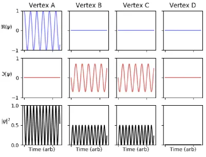
Let us now demonstrate the nature of destructive and constructive interference in the

language of graphs. Let a _∈R be a varying parameter, and consider the graphs

Gc=

1 1

1

a

(1.83)

Gd=

1 1

1

−1

a

, (1.84)

where any edge with weight dependent onais coloured purple for the benefit of the reader.

The vertices of interest are the leftmost vertex and the vertex immediately to the left of

the rightmost vertex, which we shall denote Q and R respectively. There are two walks

of length 2 from QtoR in both graphs, but the multiplicative weights of these paths are

1 and 1 in Gc, whereas they are 1 and −1 in Gd. Thus, we expect that G2c contains an

edge of weight 2 betweenQand Rdue to the constructive interference of the two possible

paths, but in G2_d such an edge is absent due to the destructive interference of the two

paths. This edge provides the avenue through which vertex Q gains a direct dependence

on the parameter a in higher powers of Gc.

We shall now demonstrate this behaviour directly through K¨onig digraphs. Starting

(41)

walk(Gc) = 1 1 1 1 1 1 a 1 1 a , (1.85)

walk(G2_c) =

1 1 1 1 1 1 a 1 1 a 1 1 1 1 1 1 a 1 1 a , (1.86) = 2 a a

a2_{+ 2}

2 2 2 2 a 2 a a , (1.87)

⇒G2_c =

2

a2_{+ 2} a

2

a a

2 . (1.88)

We can see that there will be some power ofGcthat will contain an edge connected to

Q that depends upon a by inspection: The path QRR in G2_c has a multiplicative weight

of 2(a2_{+ 2), which will contribute to the edge between} _Q_and _R _in_G4

(42)

look no further than G3_c to find the first a-dependent edge incident on Q, as

G3_c =

4 4 2a

a2_{+ 4}

a3_{+ 2}_a

. (1.89)

The eigenstates and eigenvalues of Gc are given by

γ =√a4_{+ 16}

β± =a2 −γ ±4, δ± =a2 +γ±4

vc,1 =

0 ₋ √1 2

1 √

2 0 0

λc,1 = 0 (1.90)

vc,2 ∝

δ−

√

β+

−2γ−

β+

−2γ−

β+

−√β+ √

2 a

λc,2 =−

p

2β+ (1.91)

vc,3 ∝

−δ−

√

β+

−2γ+ β+

−2γ−

β+ √ β+ √ 2 a

λc,3 =

p

2β+ (1.92)

vc,4 ∝

−β−

√

δ+

2γ+ δ+

2γ+ δ+ √ δ+ √ 2 a

λc,4 =−

p

2γ+ (1.93)

vc,5 ∝

β−

√

δ+

2γ+ δ+

−√δ+ √

2 a

λc,5 =

p

2γ+. (1.94)

The zero eigenstate solely occupies the two middle vertices due to their symmetry:

Gc is invariant under a swapping of them. However, in all other eigenstates, the (0th)

component corresponding to vertex Q have components that are all functions of a.

Let us now divert our attention to Cd. No power of Gd (and, by extension, no

poly-nomial of Gd) ever connects the vertices Q and R, demonstrated with

walk(Gd) =

(43)

walk(G2_d) = 1 1 −1 −1 1 1 a 1 1 a 1 1 −1 −1 1 1 a 1 1 a , (1.96) = 2 − a −a

a2+ 2 2 2 a2 a a , (1.97)

G2_d =

2

a2_{+ 2}

a2

a

−a

, (1.98)

G3_d =

2 2

a2+ 2

−(a2_{+ 2)}

a(a2_{+ 2)} , (1.99)

G4_d =

4

a2_{+ 4}

(a2_{+ 2)}2

a2₍_a2_{+ 2)}

−a2

a(a2+ 2)

−a(a2_{+ 2)}

(44)

G5_d =

4 4

(a2_{+ 2)}2

−(a2_{+ 2)}2

a(a2_{+ 2)}2 , (1.101)

Clearly the even powers, which are simply integer powers ofG2

d, leave vertexQisolated from the rest of the graph. Upon multiplying these by G, each contribution of a into an

edge connected to Q is cancelled out by an alternate path. The opposing signs between

the intermediate vertices and vertex R on every power of Gd prohibit any interactions

betweenQand R, thus any eigenstate with amplitude on Qmust be entirely independent

of a.

Indeed, the eigenstates and eigenvalues of Gd are

v1 =

1 2

−√2 1 1 0 0

λ1 =−

√

2 (1.102)

v2 =

1 2

√

2 1 1 0 0

λ2 =

√

2 (1.103)

v3 =

1

p

2a2₍_a2₋_{1) + 4}

0 a ₋a a2₋₂ _a2

λ3 =−

√

a2_{+ 2} _(1.104)

v4 =

1

p

2a2₍_a2₋_{1) + 4}

0 a ₋a a2_{+ 2} _a2

λ4 =

√

a2_{+ 2} _(1.105)

v5 =

1

√

2a2_{+ 4}

0 ₋a a 0 2

(45)

Chapter 2 Microscopic viewpoint

Introduction

As shown in section 1.5, eigendecomposition generally explores macroscopic properties of a system: a perturbation of an edge can have an impact on eigenstate components

corresponding to vertices far away. We have also seen that a parent graph’s macroscopic properties can be linked to those of a child graph, such that the child is achieved through some polynomial of the parent∗.

One key property of our graph algebra is that it can provide an intuitive graphical

insight into howmicroscopic properties of a graph can impact those of its polynomials; we have already seen a glimpse of this with the destructive interference demonstrated in

sec-tion 1.5.2, where even powersG2n_{exhibit a disconnect between some of the neighbouring}

vertices in G.

Of course,G was chosen specifically for this reason. How, then, does one construct a

∗_{There exist polynomials} _p₍_G_{) =} _G_{, such as} _p _{= 1 and} _p ₌ _f _{+ 1, where} _f _is _G_{’s characteristic}

(46)

G for which p(G) has some required local properties?

This section takes a pedagogical approach to introducing a toolkit which can be used

for such a purpose, starting from the simplest graphs and working up to those with more

complexity.

2.1 Polynomials and loop edges

Consider a graph S1(A) comprising a single vertex with a loop edge of weight A

S1 =

A

, walk(S1) = A , adj(S1) = (A). (2.1)

This graph admits a single eigenstate v = (1) with eigenvalue λ=A.

We can trivially see that the following properties are obeyed:

S1(A) +S1(B) =S1(A+B) (2.2)

aS1(A) =S1(aA) (2.3)

S1(A)n=S1(An), (2.4)

thus the polynomial is directly applied to the loop edge weight

P(S1(A)) =S1(P(A)) (2.5)

A graph with multiple disjoint vertices is impacted in the same way: such a graph can

be expressed as the outer sum

(47)

and the polynomial P(S) operates on the component graphs independently as

P(S(A, B, . . .)) =P(S1(A)⊕S1(B)⊕. . .) (2.6)

=P(S1(A))⊕P(S1(B))⊕. . . (2.7)

=S1(P(A))⊕S1(P(B))⊕. . . (2.8)

=S(P(A), P(B), . . .) (2.9)

P A B C . . .

!

= P(A) P(B) P(C) . . . (2.10) Thus, if a polynomial P(G) of any graph G exists which reduces it into a set of

disconnected vertices, then any child ˜P(P(G)) for some polynomial ˜P is also disconnected,

and the loop edges are directly modified by ˜P.

2.2 Edge modification

Consider a graph S2(A, B;tAB, tBA) comprising two vertices with loop edges of weight A

and B, an edge from the first vertex to the second with weighttAB, and from the second

to the first with weight tBA.

S2 = _A _B

tAB

tBA , walk(S2) = A B

tAB

tBA

, adj(S2) =



  

A s

t B 

  

(2.11)

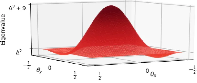
The two eigenvalues λ± of S2(A, B;tAB, tBA) satisfy

λ±=µ±

p

∆2₊_t

ABtBA µ= 1

2(A+B) ∆ =

1

(48)

The trivial addition and scalar multiplication goes along the same lines as in section 2.1

S2(A, B;tAB, tBA) +S2(A0, B0;t0AB, t 0

BA) =S2(A+A 0

, B+B0;tAB+t0AB, tBA+t0BA)

(2.13)

aS2(A, B;tAB, tBA) =S2(aA, aB;atAB, atBA), (2.14)

but multiplication is somewhat more involved. Let us begin with a squaring operation

walk(S2)2 =

A

B

B tAB

tBA

tAB

tBA

= (A2₊_tBAtAB₎

(A+B)tAB

(A+B)tBA

(B2₊_tABtBA₎

(2.15)





A B

tAB

tBA



 

2

= (A2₊_tBAtAB₎ ₍_B2₊_tAB_tBA₎

(A+B)tAB

(A+B)tBA

(2.16)

S2(A, B;tAB, tBA)2 =S2 A2 +tBAtAB, B2+tABtBA; (A+B)tAB,(A+B)tBA

.

(2.17)

As in section 2.1, the weight of the loop edges is modified through the polynomial

p : x_→ x2_{, but an extra term} _t

ABtBA is introduced. The weight of the edge linking the two vertices has also been changed. From the walk graph approach, the new loop edges

(49)

• Remaining in place for two steps

• Walking to the other vertex and back

and the new edges correspond to the walks

• Remaining in place, then walking to the other vertex.

• Walking to the other vertex, then remaining in place.

An important special case of this result is that ofA+B = 0, where the edge between

vertices A and B reduces in S₂2, separating the resulting graph into two independent

graphs of a single vertex each.



  

β −β

tAB

tBA



  

2

= β

2₊_tBAtAB _β2₊_tABtBA

(2.18)

= β

2₊_tABtBA ⊕ β

2₊_tAB_tBA

, (2.19)

or, equivalently,

S2(β,−β;tAB, tBA) 2

=S2 β2 +tBAtAB, β2+tABtBA; 0,0

(2.20)

=S1 β2 +tABtBA

⊕S1(β2+tABtBA) (2.21)

All configurations of S2 can be brought into this form through a subtraction by the

mean loop edge weight, and thus there exists a second order polynomial for eachS2 which

eliminates the edge between the two vertices

(50)

(S2(A, B;t)−µ)2 =S2(A, B;tAB, tBA)2−2µS2(A, B;tAB, tBA) +µ2 (2.23)

=S2 ∆2+tABtBA,∆2+tABtBA; 0,0

(2.24)

Thus, given

P :X _→X2 ₋2µX +µ2,

P :S2(A, B;tAB, tBA)→S1(∆2+tBAtAB)⊕S1(∆2+tABtBA). (2.25)

S1(∆2+tABtBA) has a single eigenvalue ∆2+tABtBA, and the direct sum of two such

graphs thus has two eigenvalues of the same value ∆2₊_t

ABtBA. As we have seen, we can solve

P(λ) = ∆2+tABtBA

to retrieve the eigenvalues λ± of S2

0 =λ2₋2µλ+µ2₋∆2₋tABtBA

λ =µ_± 1

2

p

4µ2₋₄_µ2_{+ 4∆}2_{+ 4}_t ABtBA

=µ_±p∆2₊_t

ABtBA,

in agreement with eq. (2.12).

This should come as no surprise, because (through the Cayley-Hamilton theorem) a

graph G solves its own characteristic equationCG

CG(G) = 0, (2.26)

and, in this case,

(51)

This graph demonstrates our second principle: polynomials can act to remove edges

between connected vertices. In two-vertex graphs, this is always achievable through some

polynomial, though larger graphs might exhibit more complex interactions that cannot

be broken down in this manner. The distinguishing feature is whether or not the graph

is what we shall call pseudo-bipartite, that is, whether the vertices can grouped into two sets such that no vertex in one set has an edge to any other vertex in the same set other than itself, and such that the loop edge weights of all vertices in such a set are identical. In this case, subtracting the mean µ of the two sets’ loop edge weights from the graphG

provides a graph G₋µ in which the two vertex sets have equal but opposite loop edge

weights.

Through the mechanism described in this section the square (G₋µ)2 _{of such a graph}

is devoid of edges between vertices of different sets, such that the sets can be separated.

In some graphs, then, simple polynomials can result in multiple independent graphs

which can be analysed in isolation to build a picture of the original graph, as we shall

exploit in section 3.4. In some other graphs, a child system may exhibit topological

defects, as explored in chapter 4, with signatures of topological behaviour appearing in

the eigenspectrum of the parent system.

2.3 Joining next-nearest neighbours

As well as eliminating an edge between nearest neighbours (those reachable with a walk of length 1), we can introduce an edge between next-nearest neighbours (those reachable with a walk of length 2). At least three vertices are needed, so we begin with a quick

overview of three-vertex graphs and move on to a chain.

(52)

let us call this graph S3(A, B, C;tAB, tAC, tBA, tBC, tCA, tCB), comprising three vertices,

A, B, C with loop edges of weight A, B, C, connected through edges tij (where i, j are

distinct vertices labelled by their weight A, B, C)

S3 =

A B C tAB tBA tCB tBC tCA

tAC walk(S3) =

A tAB tAC tBA B tBC tCA tCB C, (2.28)

adj(S3) =

       

A tBA tCA

tAB B tCB

tAC tBC C

        . (2.29)

S3 squares as

S3(A, B, C, tAB, . . .)2 =S3(A0, B0, C0, t0AB, . . .) (2.30)

with

X0 =X2+tXYtY X+tXZtXZ (2.31)

t0_XY =tXY(X+Y) +tXZtZY (2.32)

for all X, Y, Z _{∈ {}A, B, C_}, X ₆=Y ₆=Z

Now we shall move on to a special case: the chain L3(A, B, C, tAB, tBA, tBC, tCB)

(53)

L3 =S3(A, B, C, tAB,0, tBA, tBC,0, tCB) (2.33)

=

A

B C

tAB

tBA

tCB

tBC

(2.34)

walk(L3) = A

tAB tBA

B

tBC tCB

C (2.35)

Although L3 has a disconnect between A and C, they become connected in (L3)2 by

edges of weight tABtBC, tCBtBC.

(L3(A, B, C))2 =

A2₊_tABtBA

B2₊_tBAtAB₊_tBCtCB _C2₊_tCBtBC

tAB(A+B)

tBA(A+B)

tCB(B+C)

tBC(B+C)

tCBtBC

tABtBC _,

(54)

As these edges are single term multiples of existing bonds, there does not exist a

config-uration of L3 which does not exhibit an edge between A and C in its square, apart from

those with at least one absent edge. Furthermore, the edges between A and B can be

eliminated in the square if A+B = 0 and those between B and C if B +C = 0

(L3(A,−A, C)) 2

=

A2₊_tABtBA

A2+tBAtAB+tBCtCB A2+tCBtBC

tCB(C₋A)

tBC(C₋A)

tCBtBC tABtBC

(2.37)

If A = C, B = ₋A, then both of these conditions are met and the only remaining edges

will be between A and C

(L3(A,−A, A))2 =

A2₊_tABtBA

A2₊_tBAtAB₊_tBCtCB _A2₊_tCBtBC

tCBtBC tABtBC

(2.38)

Note thatL3(A,−A, C)2 is also a chain, and upon swapping the labelling ofB and C

(55)

L3(A,−A, C)∼L3

A2+tABtBA, A2+tCAtAC, A2+tBAtAB+tBCtCB;

tABtBC, tCBtBC, tCB(C−A), tBC(C−A)

(2.39)

2.4 Interference

We have now seen that next nearest neighbours can become connected by an edge under

a second power, and that this is unavoidable in a three-site chain without absent edges. It

is, however, possible to produce a graph in which the second power does not exhibit

next-nearest edges, as we have seen in section 1.5.2. The trick is to introduce an additional

intermediate vertex with edges chosen such that the multiplicative path between two

next-nearest neighbours cancels out through destructive interference.

Consider, then, a graphC4 in the form of a square

C4 =

A B C D tAB tBA tCD tDC tAC

tCA tDB tBD adj(C4) =

           

A tBA tCA 0

tAB B 0 tBD

tAC 0 C tDC

0 tBD tCD D

           

walk(C4) =

(56)

SquaringC4 results in a new graph with edges

A0 =A2+tBAtAB +tCAtAC (2.41)

B0 =B2+tDBtBD+tABtBA (2.42)

C0 =C2+tCAtAC+tDCtCD (2.43)

D0 =D2+tCDtDC+tDBtBD (2.44)

t0_XY =tXY(X+Y), (2.45)

where tXY are existing edges in C4, and four additional edges connecting the next

nearest neighbours

t0_AD =tBDtAB+tCDtAC (2.46)

t0_DA =tBAtDB+tCAtDC (2.47)

t0_BC =tACtBA+tDCtBD (2.48)

t0_CB =tABtCA+tDBtCD (2.49)

We can cancel out the vertex between the next nearest neighbours by restricting edges

such that the terms above cancel. For example, with

tAB =−α tBD =

tCDtAC

α (2.50)

tBA=−β tDB =

tCDtAC

β (2.51)

the edges t0_AD (through eq. (2.50)) and tBA (through eq. (2.51)) are cancelled out.

(57)

tCD =γ tDC = αβ γ such that                 A B C D −α −β γ αβ γ tAC

tCA tACγ

α tCAα

γ                 2 =

A2 _B2

C2 _D2

−α(A+B)

−β(A+B)

γ(C+D)

αβ

γ (C+D) tAC ( A + C )

tCA

( A + C ) γ

tAC α

( B + D ) αt C A γ ( B + D )

+ (tACtCA+αβ), (2.52)

where for notational ease we imply the final term multiplies with the identity.

Thus, along with a choice ofA, B, C, D, tAC and tCA, we have the choice of three free

parameters α, β, δ from which to produce a graph which exhibits destructive interference

between (Aand D) and (B and C), resulting in another C4, after raising to the power 2.

As we have seen in section 2.2, we can separate neighbouring vertices by providing

them with opposing loop weights. For example,

• A= ∆, B =₋∆ separates A and B,

• A = ∆, B =₋∆, C = ∆, D =₋∆ separates A and B and C and D, resulting in a

separable graph of two S2 subgraphs.

• A= ∆, B =₋∆, C =₋∆, D = ∆ separates all four sites, resulting in four isolated

New algebraic relationships between tight binding models