Tensor networks and geometry for the modelling of disordered quantum many body systems

warwick.ac.uk/lib-publications

the modelling of disordered quantum many-body systems. IOP Computational Physics Group newsletter . (Submitted).

Permanent WRAP URL:

http://wrap.warwick.ac.uk/81876

Copyright and reuse:

The Warwick Research Archive Portal (WRAP) makes this work of researchers of the University of Warwick available open access under the following conditions.

This article is made available under the Creative Commons Attribution 4.0 International license (CC BY 4.0) and may be reused according to the conditions of the license. For more details see: http://creativecommons.org/licenses/by/4.0/

A note on versions:

The version presented in WRAP is the published version, or, version of record, and may be cited as it appears here.

Tensor Networks and Geometry for the Modelling of Disordered Quantum Many-Body Systems

Andrew M. Goldsborough1, 2,∗ and Rudolf A. R¨omer2,†

1_{Max Planck Institute for Quantum Optics,}

Hans-Kopfermannstr. 1, D-85748 Garching, Germany

2_{Department of Physics and Centre for Scientific Computing,}

The University of Warwick, Coventry, CV4 7AL, United Kingdom

(Dated: August 9, 2016)

I. INTRODUCTION

At its most fundamental level a quantum many-body system can be defined by a Hilbert spaceH and a HamiltonianHdescribing the evolution of states inH. But with∼21023states for just a single mole of, e.g., spin-1/2 particles, computing ground states and excitations remains a formidable challenge. Fortunately, advanced numerical methods have been developed in the last decades to tackle the problem. Whilst density-functional theory, dynamical mean-field theory, quantum Monte Carlo and their variants and extensions have allowed us to study systems with hundreds – and sometimes thousands – of atoms in three dimensions, large strongly correlated systems are more problematic. However, much has been learned in low dimensional systems by applying concepts from quantum information to many body physics. At the heart of this understanding lies the realization that not all states in Hare equal in terms of their entanglement properties. For a general state inHthe entanglement entropyS_A|B scales as thevolume of subsystem. However, for ground states of gapped systems, the entanglement scales as the area of the boundary separating the subsystems. This is the famous area law for entanglement entropy [1–3]. It suggests that much of the low energy physics is likely to be well described by a much smaller, area law satisfying subset of H. The success of tensor network methods is down to their ability to capture the entanglement described by the area law and provide a variational ansatz within the space of area law satisfying states [4]. The simplest tensor network, the matrix product state (MPS), is at the heart of the density matrix renormalisation group (DMRG) algorithm, accepted to be the most accurate approach for the numerical study of strongly correlated 1D systems [5]. In 2D, one has to use more sophisticated tensor networks such as projected entangled pair states (PEPS) to make progress.

The area law for SA|B in quantum-many body systems was foreshadowed in the theory of black hole thermodynamics. It had been found [6, 7] that black holes have a thermal Bekenstein-Hawking entropy SBH = A_4Gh, that scales with the surface area Ah of the black hole horizon; Gis Newton’s gravitational constant. ForSA|B, Ryu and Takayanagi [8] suggest a similar extension in the context of the so-called AdS/CFT correspondence, i.e. the duality between quantum gravity on aD+ 2 dimensional Anti-de Sitter (AdS) spacetime and a conformal field theory (CFT) defined on its D+ 1 dimensional boundary [9]. The entanglement entropy of a region A of the CFT is related to the size of the surface with smallest area, or minimal surface γA, within the AdS bulk that separates A from the rest of the system. This is shown pictorially in fig. 1. In condensed matter systems, AdS/CFT can provide a geometric interpretation of the renormalization group (RG) approach. The additional holographic dimension can be interpreted as a scale factor in the RG coarse graining [10]. This analogy givesS_A|B =

A_γA

4G(_ND+2), whereAγA is the area of the minimal

∗

andrew.goldsborough@mpq.mpg.de †

minimal surface

holographic dimension

FIG. 1. A diagrammatic representation of the AdS/CFT correspondence, showing a (D+ 1) dimensional CFT on the boundary of a (D+ 2) dimensional AdS spacetime. The entanglement entropy of a regionAof the CFT is proportional to the minimal surfaceγA that separatesA from the remainder of the CFT.

surfaceγAand G(_ND+2) is Newton’s constant in D+ 2 dimensions. As we shall see, these concepts underpin the success of tensor networks that satisfy the area law and beyond.

For disordered and interacting systems, the variational refinement of tensor networks can al-ready be too costly and has to be balanced with the need to additionally average of many, sometimes thousands of disorder realizations. As we will show here, instead of variationally refining a partic-ular tensor network, a strategy that self-assembles the tensors according to a physically motivated, realisation-specific disordered network provides a viable alternative strategy.

II. MATRIX PRODUCT STATES

Consider a quantum system with basis states |↑i and|↓i for each site in a system withL sites. Simpleproduct states can be formed as tensor product of the bases [11], for example|↑i ⊗ · · · ⊗ |↑i. For, e.g. L= 2, any state can be written as a superposition of all possible two site product states,

|Ψi= (u1|↑i+d1|↓i)⊗(u2|↑i+d2|↓i) =

X

σ1,σ2

Cσ1,σ2|σ1i ⊗ |σ2i, (1)

whereσi can be ↑or↓,ui,di are numerical coefficients andCσ1,σ2 is a two component tensor with elements

C=

u1u2 u1d2

d1u2 d1d2

. (2)

Product states such as (1) have bases independent of each other and the expectation values factorise. On the other hand, entangled states such as

|Ψi= √1

2(|↑i ⊗ |↓i − |↓i ⊗ |↑i) (3)

do not have factorising expectation values. The maximally entangled state (3) would require a tensor of the form

C≡

σ2 =↑ σ2=↓

σ1=↑ 0 1/

√ 2

σ1=↓ −1/

√

2 0

= √1 2

0 1

−1 0

!

3

(a) (b)

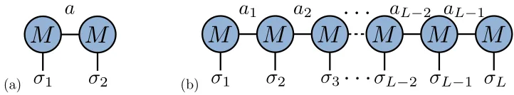
FIG. 2. Diagrammatic representation of (a) the two site MPS in eq. (6) and (b) the general Lsite MPS of eq. (7). The circles represent the M tensors and the lines are the tensor indices. The horizontal lines represent the bond indices, the vertical lines the physical indices.

which cannot be described by the coefficientsu1,d1,u2 andd2 in eq. (2). Instead, let us introduce

matrices [12],

M1 =

1 4 √ 2 1 0 0 1 !

, M2 =

1 4 √

2

0 1

−1 0

!

. (5)

These matrices, combined using a standard matrix product, can easily produce the entangled state

Cσ1,σ2 =

X

a

[M1]σa1[M2]σa2 ⇒ C= 1 √ 2

0 1

−1 0

!

, (6)

as desired. The a index introduces entanglement between the two states and can be thought of as a form of bond. Note that we have chosen the upper and lower placement of the indices for later convenience. Eq. (6) defines the simplest matrix product state (MPS). It can be expressed diagrammatically as in fig. 2(a), where the matrix is drawn as a circle and each index is represented by a line orleg. The matrix multiplication, or more generally tensor contraction, is shown by joining the lines that represent the summed over index. These diagrammatic representations of the state become very convenient for larger and more complicated tensor networks and are commonplace in the literature.

A general wavefunction on a lattice of L sites can be written as |Ψi=P

σ1,...,σLCσ1...σL|σ1i ⊗ · · · ⊗ |σLi. As with the two site case, the Cσ1...σL tensor can be split into a series of local tensors with connections to their neighbours that allow the inclusion of entanglement. When away from boundaries each site has two neighbours thus the tensors at each site have three indices; one for the site basis and one for each neighbour. In full the wavefunction takes the form

|Ψi= X

σ1,...,σL X

a1,...,aL−1

Mσ1

a1M

σ2

a1a2. . . M

σL

aL−2aL−1M

σL

aL−1|σ1, . . . , σLi, (7)

where |σ1. . . σLi ≡ |σ1i ⊗ · · · ⊗ |σLi and Maiσi−1ai ≡ [Mi]

σi

ai−1ai. The σi indices label the spins of the basis and are known as the physical indices, whereas theai are the bond, virtual orauxiliary indices. To draw a distinction between the two index types, it is convention to have the physical σi as upper indices, thus giving the standard form of an MPS [5]. As before, the MPS can be represented diagrammatically as a chain of circles connected horizontally by the bond indices and with the physical indices drawn vertically as in fig. 2(b). Note that (7) corresponds to a state with open boundary conditions (OBCs) as is evident from the special tensors Mσ1

a1 and M

σL

aL−1 at the sites 1 andL.

The MPS (7) is an exact representation of any state in H. When increasing site index i up to the centre of the chain, the size of each M_aiσi_−1ai increases. For example when i = L/2 the

dimensions of the MPS tensor are [d, dL2−1, d

L

2], where d is the dimension of the site basis, e.g.

(a) (b)

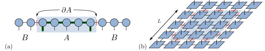
FIG. 3. (a) For an MPS a regionA(shaded blue) is bounded by two bonds, denoted by red lines. If the size ofAis increased the number of bonds stays at 2. The bold green line highlights the minimum path between two sites. (b) A PEPS on a square lattice, where the PEPS tensors are blue squares, the virtual indices are in the plane, and the physical indices are those pointing up. As before, the region under consideration is highlighted in blue and the bonds that separate it from the rest of the system are shown by red lines. Here the boundary scales as 4Land is therefore area law conserving.

expected when all of the information is preserved. By limiting the size of the bond indices, known as setting thebond dimension χ, one truncates the size of the Hilbert space allowing much larger system sizes to be computationally tractable. Settingχ also controls the amount of entanglement that the wavefunction (7) can have. Due to the fact that ground states of gapped Hamiltonians satisfy the area law, and therefore have relatively little entanglement, setting a finiteχstill allows for an accurate description of the wavefunction. For example, while exact diagonalisation is usually limited toL∼30 sites [13], the MPS approach can study many hundreds of sites withχ∼ O(103) [14]. The MPS can be used as a variational ansatz by sweeping back and forth across the chain choosing the contents of each M_aiσi_−1ai that minimises the energy. This variational MPS algorithm is often referred to as DMRG, despite the fact that the original DMRG algorithm [15] does not use an MPS. A full discussion of MPS based DMRG can be found in reference [5].

III. TENSOR NETWORKS

A. The Area Law for Entanglement Entropy

As highlighted in the introduction, the area law states that the entanglement entropy for ground states in gapped quantum many body systems scales with the boundary of a subsystem rather than the volume. This means that these ground states are significantly easier to simulate on a classical computer than generic states. For tensor networks the boundary is quantified by the number of bonds nA connecting region A to the environment B. The reasoning behind this measure is that if all of the tensors are identical, with a bond dimension χ the maximum contribution to the entanglement entropy per bond is log₂(χ). Evenbly and Vidal [16] go further to suggest that for most cases of homogeneous tensor networks the entanglement per bond is approximately 1, hence S_A|B ≈nA. The boundary of a region in a 1D system is simply two points and does not increase when the region is expanded. An MPS has these same properties; the number of bonds that one would have to cut to separate region AfromB is 2 and does not change if the size ofA is altered, as shown in fig. 3(a). The fact that the MPS has the same entanglement properties as the ground state of a gapped 1D system makes it an ideal variational ansatz for such problems and gives a reason for the excellent scaling for these systems.

5

MPS is insufficient as a variational ansatz for this system. An area law conserving ansatz would be a tensor network where all sites are connected to their four neighbours to match the lattice geometry, as shown in fig. 3(b). This tensor network is known as a projected entangled pair state

(PEPS) and is can be viewed as natural 2D extension of the MPS [19, 20].

B. Beyond the Area Law

Tensor networks, particularly the multi-scale entanglement renormalisation ansatz (MERA) [21, 22], can be seen as a coarse grained embodiment of AdS/CFT [16, 23]. The structure of MERA, shown in fig. 4(a), is made up of disentanglers (green squares) and isometries (pink triangles). The intuitive argument behind its construction is that the disentanglers remove short range entanglement so that the isometries can then remove degrees of freedom that are no longer coupled to the system. The network is self-similar in the way that at each level of coarse graining the network looks the same. This direction of coarse graining, perpendicular to the physical lattice, is the extraholographic dimension.

Just as with MPS and PEPS, the minimal surfaceγAis found by counting the minimum number of bonds that have to be cut to separate one region from the rest of the system. Take, for example, a region comprised ofLsites within a MERA as shown in fig. 4(a). The minimum number of bonds (red lines in fig. 4(a)) nA ≈ log(L), which matches the entanglement scaling of critical systems [16]. As an extension of this, it was shown [24, 25] that in the continuum limit of MERA it has a metric that matches the properties of AdS/CFT.

In addition to entanglement entropy, similar arguments hold for two-point correlation functions [16, 23]. The asymptotic scaling of correlation functions should be

CTN(x1, x2)∼e−αDTN(x1,x2), (8)

whereDTN is the path with the minimum distance orgeodesicconnecting points x1 andx2 within

the tensor network. For MPSDMPS=|x2−x1|, as shown as the bold line in fig. 3(a). Hence

CMPS(x1, x2)∼e−αDMPS(x1,x2) =e−|x2−x1|/ξ, (9)

whereξ is the correlation length. MERA, on the other hand has path lengths that scale logarith-mically with separation ofx1 and x2 (DMERA(x1, x2)∝log2(L)), as shown in fig. 4(a). Thus

CMERA(x1, x2)∼e−αDMERA(x1,x2)=|x2−x1|−q, (10)

recovering the power law decay profile characteristic of critical systems.

IV. STRUCTURALLY INHOMOGENEOUS TENSOR NETWORKS

(a) (b)

Lattice Dimension

FIG. 4. (a) Tensor network diagram of a MERA with periodic boundary conditions where the green squares aredisentanglers, pink triangles areisometries and the blue circle is the top tensor. A region of the network corresponding to Lsites is highlighted in blue, where the bonds making up the minimum surface are highlighted by the red lines. The bold green line highlights a geodesic connecting two points on the lattice. (b) The SDRG algorithm as a TTN for a chain of L = 20 sites. Shapes and lines are as in (a). Lattice and holographic dimensions are indicated by the dashed arrows.

to the removal of local degrees of freedom in MERA and also suggests the possible usefulness of concepts from AdS/CFT for disordered spin chains.

The SDRG method was extended by Hikihara et. al. [30] to include higher states at each decimation, in the spirit of Wilson’s numerical renormalisation group [31] and DMRG [15]. This method therefore decomposes the system into blocks rather than larger spins allowing for more accurate computation of, e.g., spin-spin correlation functions. The more states that are kept at each decimation the more accurate the description and it is exact in the limit of all states kept. This numerical SDRG amounts to a coarse-graining mechanism that acts on the operator. We show in reference [26] that it is equivalent to view this as a multi-level tensor network wavefunction acting on the original operator. The operators that coarse-grain two sites to one can be seen as

isometric tensors orisometries that satisfyww†=116=w†w. When viewed in terms of isometries, the algorithm can self-assemble a tensor network based on the disorder of the system. When written in full, it builds an inhomogeneous binary tree tensor network (TTN) as shown in fig. 4(b). We shall henceforth refer to this TTN approach to SDRG as tSDRG. For a full description of the algorithm see reference [26].

A. Correlation Functions

The correlation functions for a strongly disordered Heisenberg chain are expected to disorder-average to a power-law decay with power|x2−x1|−2 [29]. As discussed in section III B, correlation

functions in tensor networks scale as e−αD(x1,x2)_{, where D(x}

1, x2) is the number of tensors that

connect site x1 tox2 [16], for exampleD(6,13) = 5 in fig. 4(b) highlighted in green. tSDRG has a

holographic geometry based on a random TTN, with average path lengthhDTTNi ≈log|x2−x1|,

i.e. scaling logarithmically with distance. This makes it ideally suited to capture the desired power law decay

hh~sx1·~sx2ii ∼e

−αhDTTN(x1,x2)i_∼e−αlog|x2−x1|_{∼ |x}

7

(a)

100 101 102

| x 2 - x1 |

10-3 10-2 10-1 100

〈〈

sx1

.

sx2

〉〉

tSDRG χ=10 5.81 exp[-0.63D

TTN] ~| x

2 - x1 | -2

1 10 100

| x

2 - x1 |

0 5 10 15 20 DTTN D

TTN(x1 , x2)

2.94 ln |x

2 - x1| + 3.02

(b)

20 40 60 80 100 120 140 160

| x 2 - x1 |

10-4 10-3 10-2 10-1 100 〈〈

sx1

.

sx2

〉〉

tSDRG χ=10

1.67 〈 exp[-D

TTN] 〉 0.69

~| x

2 - x1 | -2

~| x

2 - x1 | -1.78

FIG. 5. (a) Reproduced from [26]. Correlation function for L= 150 averaged over 2000 samples for the direct calculation ofhh~sx1·~sx2ii(black circles) and also via the holographic approach (11) usingDTTN(dashed

red line with error of mean indicated by the grey shading) such thathh~sx1·~sx2ii ≈(5.81±0.93)exp[−(0.62±

0.02)DTTN]. The expected thermodynamic scaling |x2−x1|−2 is also shown (solid blue line). Inset: The

holographic path lengthDTTN connecting sites x1 and x2 averaged over the 2000 TTNs (black) and a fit

in the logarithmic regime (red). (b) Rescaled correlation function to remove odd-even effects on a semi-log plot. The expected thermodynamic scaling is shown as a solid blue line. The fitted scaling factor from (a) is plotted as a solid green line. The red line indicates the alternative holographic fitting with

hh~sx1·~sx2ii ≈(1.67±0.10)hexp[−DTTN]i

(0.69±0.01)_.

In fig. 5(a), we show the behaviour of hh~sx1 ·~sx2ii, with hh·ii denoting quantum and disorder averages, computed directly as well as its holographic estimate based on (11). We find that the behaviour for|x2−x1| 1 and|x2−x1|< L/2 is indeed very similar for both approaches. We find

that in the indicated distance regime, both measures ofhh~sx1·~sx2iiare consistent with the expected r−2 behaviour. For|x2−x1|&L/2 we see that the boundaries lead to an upturn ofhh~sx1·~sx2iifor both direct and holographic estimates. This upturn is a result of boundary effects and can easily be understood in terms of the holographic TNN; for|x2−x1| ≥L/2, the average path length in the

tree decreases [32]. In the inset of fig. 5(a) we show the distance dependence ofDTTN withχ= 10.

For|x2−x1|< L/2, the data can be described by as linear behaviour in log|x2−x1|. We observe

that as Lincreases, the resulting value of the scaling power aalso increases towards the expected value of 2. We have also checked that the differences between χ = 10 and 20 remain within the error bars and hence we use χ = 10 for calculations of hh~sx1 ·~sx2ii in fig. 5(a). We further note that fig. 5(a) shows a clear difference in the correlation function between even and odd distances, due to the fact that singlets can only form with nearest neighbours on each coarse graining scale. While eq. (11) neatly describes the power law behaviour of the data, a more accurate ansatz should be

hh~sx1·~sx2ii 'Ahe

−DTTN(x1,x2)_ia_{. (12)}

We plot the fit to (12), along with the correlation data rescaled to remove the even-odd variation [33], in fig. 5(b). This shows thathh~sx1·~sx2ii ≈(1.67±0.10)hexp[−DTTN]i

(0.69±0.01)_{is a remarkably}

accurate fit to the data for all length scales. Our result implies that the majority of the correlation information is stored in the structure of the TTN rather than the contents of the tensors.

B. Entanglement Entropy

In general the entanglement entropy SA|B =−TrρAlog2ρA is difficult to compute as the size of

represen-(a)

0 10 20 30 40 50

L

B

1.5 2

SA,B

0 10 20

%failed

(b)

0 10 20 30 40 50

L B 0.5

1 1.5 2

SA,B

, S

A,B

/n

A

FIG. 6. Reproduced from [26]. (a) The entanglement entropySA,B (black) averaged over 500 samples as

a function of the size of a block LB placed in the middle of a chain with L = 50 forχ = 10. The fitting

(red, solid line) givesSA,B= (0.22±0.02)log2LB+ (1.12±0.05) forLB ≤25, above which finite size effects

dominate. The grey shaded region indicates the accuracy of the fit. The (green) dashed line shows the entanglement scaling from ref. [34] with the vertical position fitted to the pointLB = 2. The straight black

lines are a guide to the eye only. At the bottom, we show the failure rate in percent (crosses) for different

LB. (b) Entanglement entropy S (black circles) and entanglement entropy per bondS/nA(red diamonds)

for left-right bipartitions A|B (top, open symbols) and central blocks A,B (bottom, filled symbols) with

χ= 10. The entanglement per bond saturates to 0.47±0.02 for bipartitions and 0.48±0.02 for blocks (grey shaded regions).

tation of tSDRG gives an alternative means of finding S_A|B for any bipartitions A and B of the

system. In a similar manner to the correlation functions, the geometry of the tensor network is related to its ability to capture entanglement. As discussed in section III B, SA|B is proportional

to the minimum number of indices, nA, that one would have to cut to separate a block A of spins from the rest B of the chain [16, 26]. For the TTN the position of the block in the chain alters the number of indices that have to be cut to separate it from the rest of the system. This suggests that there are spatial regions in the chain that are more and less entangled, which is likely to be true for a strongly disordered spin chain.

In refs. [34, 35], Refael and Moore calculate a block entanglement SA,B in the random singlet

phase and show that it scales as (ln[2]/3) log₂LB where region B is a block of extent LB in the

centre of the spin chain. We show the resultingSA,B in fig. 6(a). The figure clearly indicates that

finite size effects become prevalent for largeLB, so we fit forLB≤L/2 only. The resulting scaling

behaviourSA,B≈(0.22±0.02)log2LBis fully consistent with previous results [35]. We also examine

the entanglement entropy per bond,S/nA, of a TTN for both left-right bipartitions A|B and blocks

A,B withχ= 10 when averaging over 500 disorder configurations withL= 50. Figure 6(b) shows that away from the boundaries S/nA saturates to the same constant 0.47±0.02 in both cases.

Note that forLB∼L/2, we find that up to 20% of our samples for χ= 10 lead to calculations of

SA,B consuming memory beyond 100GB and therefore fail to complete. Nevertheless, we believe

that this will not greatly change the average values ofSA,B/nAreported here as the higher failure

rate is for block sizes where boundary conditions become influential, which is supported by the calculations for smaller χ. For χ = 4 we find 0.42±0.02 for both blocks and bipartitions with a much lower failure rate (< 1%) due to the smaller size of the density matrices. This might conceivably suggest thatS/nA= 0.5 is a limiting value for larger χand L. This is consistent with

9

V. CONCLUSIONS AND OUTLOOK

The use of tensor networks within the fields of condensed matter physics and quantum infor-mation theory is becoming ever more common. MPS based DMRG is widely believed to be the most accurate method of numerically modelling 1D systems and it is being applied in increasingly complicated scenarios [4, 5]. PEPS are being used both as a numerical method and as an analytic platform to study two dimensional strongly correlated systems, particularly topological phases of matter [36, 37]. MERA and holographic tensor networks are beginning to be applied in various other fields such as in high energy physics to potentially link entanglement and gravity [38], and quantum information in the creation of holographic error correction codes [39].

There are many ways that tensor networks can aid the study of disordered systems. Although DMRG is in some ways imperfect for the modelling of disorder, it is so efficient that much can still be learned by applying it [40]. Beyond the Heisenberg and Bose-Hubbard models, there are still a myriad of possible Hamiltonians that can be examined with DMRG. A current area of intense research is many-body localisation (MBL), the generalisation of Anderson localisation to interacting many-body systems [41]. It is believed that the area law holds for all excited states in systems with MBL up to some mobility energy, unlike gapped quantum systems where only the ground state is area law satisfying [42]. This in principle should allow for an efficient MPS representation, and therefore accurate DMRG simulation, of any state in a 1D MBL spectrum. Strong disorder renormalisation techniques such as tSDRG can be used as high precision methods when disorder is strong. The method should be accurate for use with the FM/AFM disordered spin-1/2 Heisenberg model where large effective spins would be created as the renormalisation progresses [30]. Beyond spin-1/2 there have been exciting discoveries in disordered spin-3/2 Heisenberg systems, where the rich phase diagram contains topological phases as well as spin doublet and triplet phases [43]. It would be fascinating to uncover the optimal tensor network geometries in these situations.

More generally our results suggest that it might be possible to construct an algorithm that can decide autonomously on the best network geometry for a particular system under consideration. Currently the geometry in most tensor network approaches is set by hand using prior knowledge of the model. In a network that can self optimise the structure, the final geometry can become a resource for learning about the properties of the wavefunction. Perhaps with these ideas, truly scalable 2D and 3D tensor network algorithms may emerge for clean and disordered systems.

[1] M. Srednicki, Phys. Rev. Lett.71, 666 (1993).

[2] M. B. Hastings, J. Stat. Mech. Theor. Exp.2007, P08024 (2007). [3] J. Eisert, M. Cramer, and M. B. Plenio, Rev. Mod. Phys.82, 277 (2010). [4] R. Or´us, Ann. Phys.349, 117 (2014).

[5] U. Schollw¨ock, Ann. Phys.326, 96 (2011).

[6] J. Bekenstein, Lett. Nuovo Cimento Series 2 4, 737 (1972). [7] S. W. Hawking, Nature248, 30 (1974).

[8] S. Ryu and T. Takayanagi, Phys. Rev. Lett. 96, 181602 (2006). [9] J. Maldacena, Int. J. Theor. Phys. 38, 1113 (1999).

[10] J. McGreevy, Adv. High Energy Phys.2010, 723105 (2010).

[11] I. Peschel and V. Eisler, inComputational Many-Particle Physics, Vol. 739 ofLect. Notes Phys., edited by H. Fehske, R. Schneider, and A. Weiße (Springer, Berlin, Heidelberg, 2008), pp. 581–596.

[12] G. M. Crosswhite and D. Bacon, Phys. Rev. A78, 012356 (2008).

[13] N. Laflorencie and D. Poilblanc, inQuantum Magnetism, edited by U. Schollw¨ock, J. Richter, D. J. J. Farnell, and R. F. Bishop (Springer, Berlin, Heidelberg, 2004), pp. 227–252.

[20] F. Verstraete, V. Murg, and J. I. Cirac, Adv. Phys.57, 143 (2008). [21] G. Vidal, Phys. Rev. Lett.99, 220405 (2007).

[22] G. Evenbly and G. Vidal, Phys. Rev. B79, 144108 (2009). [23] B. Swingle, Phys. Rev. D86, 065007 (2012).

[24] M. Nozaki, S. Ryu, and T. Takayanagi, J. High Energy Phys.2012, 193 (2012).

[25] A. Mollabashi, M. Nozaki, S. Ryu, and T. Takayanagi, J. High Energy Phys.2014, 1 (2014). [26] A. M. Goldsborough and R. A. R¨omer, Phys. Rev. B89, 214203 (2014).

[27] S.-k. Ma, C. Dasgupta, and C.-k. Hu, Phys. Rev. Lett.43, 1434 (1979). [28] C. Dasgupta and S.-k. Ma, Phys. Rev. B22, 1305 (1980).

[29] D. S. Fisher, Phys. Rev. B50, 3799 (1994).

[30] T. Hikihara, A. Furusaki, and M. Sigrist, Phys. Rev. B60, 12116 (1999). [31] K. G. Wilson, Rev. Mod. Phys47, 773 (1975).

[32] A. M. Goldsboroughet al., arXiv:1502.07893 [math-ph] (2015).

[33] J. A. Hoyos, A. P. Vieira, N. Laflorencie, and E. Miranda, Phys. Rev. B76, 174425 (2007). [34] G. Refael and J. E. Moore, Phys. Rev. B76, 024419 (2007).

[35] G. Refael and J. E. Moore, Phys. Rev. Lett.93, 260602 (2004).

[36] T. B. Wahl, H.-H. Tu, N. Schuch, and J. I. Cirac, Phys. Rev. Lett.111, 236805 (2013). [37] D. Poilblanc, J. I. Cirac, and N. Schuch, Phys. Rev. B91, 224431 (2015).

[38] B. Swingle and M. V. Raamsdonk, arXiv:1405.2933 [hep-th] (2014).

[39] F. Pastawski, B. Yoshida, D. Harlow, and J. Preskill, J. High Energy Phys.2015, 1 (2015). [40] A. M. Goldsborough and R. A. R¨omer, EPL111, 26004 (2015).

[41] D. Basko, I. Aleiner, and B. Altshuler, Ann. Phys.321, 1126 (2006). [42] A. Chandranet al., Phys. Rev. B92, 024201 (2015).