Empirical tight-binding model for titanium phase transformations

Empirical tight-binding model for titanium phase transformations

D. R. Trinkle,1,2M. D. Jones,3,2R. G. Hennig,4S. P. Rudin,2R. C. Albers,2and J. W. Wilkins4 1_{Materials and Manufacturing Directorate, Air Force Research Laboratory, Wright Patterson Air Force Base,}

Dayton, Ohio 45433-7817, USA

2_{Theoretical Division, Los Alamos National Laboratory, Los Alamos, New Mexico 87545, USA} 3_{State University of New York, Buffalo, New York 14260, USA}

4_{Ohio State University, Columbus, Ohio 43210, USA}

共Received 26 February 2005; revised manuscript received 13 December 2005; published 28 March 2006兲 For a previously published study of the titanium hexagonal close packed共␣兲to omega共␻兲transformation, a tight-binding model was developed for titanium that accurately reproduces the structural energies and elec-tron eigenvalues from all-elecelec-tron density-functional calculations. We use a fitting method that matches the correctly symmetrized wave functions of the tight-binding model to those of the density-functional calculations at high symmetry points. The structural energies, elastic constants, phonon spectra, and point-defect energies predicted by our tight-binding model agree with density-functional calculations and experiment. In addition, a modification to the functional form is implemented to overcome the “collapse problem” of tight binding, necessary for phase transformation studies and molecular dynamics simulations. The accuracy, transferability, and efficiency of the model makes it particularly well suited to understanding structural transformations in titanium.

DOI:10.1103/PhysRevB.73.094123 PACS number共s兲: 71.15.Nc, 61.72.Ji, 63.20.⫺e, 62.20.Dc

I. INTRODUCTION

Titanium is a useful starting material for many structural alloys;1_{however, the formation of the high-pressure omega} phase is known to lower toughness and ductility.2The atom-istic mechanism of the transformation from the room tem-perature␣phase关hexagonal close packed共hcp兲兴to the high-pressure␻was recently elucidated by Ref. 3. The explication of the␣→␻atomistic transformation relied on the compari-son of approximate energy barriers for nearly 1000 different 6- and 12-atom pathways. That study required the use of an accurate and efficient interatomic potential model: In this case, a tight-binding model reparametrized using all-electron density-functional calculations.

After reparametrizing, we modify the functional form of tight binding for small interatomic distances to overcome the collapse problem. This ensures that the potential is suitable for phase transition studies and molecular dynamics simulations. The collapse problem for tight-binding models is caused by unphysically large overlap at small distances creating a low energy binding state; by modifying the functional form using short-range splining, the collapse problem can be avoided. This paper provides the details of the model used in the previous phase transformation study of Ref. 3 and describes a general solution to the collapse prob-lem.

Tight binding共TB兲is a parametrized electronic structure method for calculation of total energies and atomic forces for arbitrary structures. It is an empirical model that can reproduce density-functional results for a range of structures yet requires orders of magnitude less computational effort. The parameters of the model are determined by fitting to a database and the range of applicability is determined by comparison to structures not in the database. The end result is a model that balances three competing

properties—efficiency, accuracy, and transferability—which make it applicable to a variety of important structures.

We fit our model to total energies and electron eigenval-ues for several crystal structures over a range of volumes to produce a transferable model for the study of the ␣→␻ transformation in Ti.3 _{The potential has been successfully} used to compute and sort possible transformation pathways,4 comparing favorably with generalized gradient approxima-tion共GGA兲calculations in accuracy. Our fitting database is chosen to sample a large portion of the available phase space of parameters while constraining those parameters as much as possible. The resulting model reproduces total energies, elastic constants, phonons, and point defects; all of which are necessary for transformation modeling. The computational efficiency allows simulations of length and time scales that are inaccessible with GGA. In addition, the functional forms are modified for small distances to overcome the unphysical collapse problem; this is necessary for phase transitions and molecular dynamics which sample small interatomic dis-tances. Moreover, the modification presented is applicable to other nonorthogonal tight-binding models without modifying existing parameters, hence extending their range of applica-bility.

Section II describes tight binding as a parametrized elec-tronic structure method, the functional forms for titanium, the modifications for short distances, our fitting database, and our method of optimization. Section III gives the opti-mized parameters, and tests our model against total energies, elastic constants, phonons, and point defect formation ener-gies for ␣,␻, and body-centered cubic 共bcc兲 Ti. The point defect formation energies are used to compare our param-eters to those of Mehl and Papaconstantopoulos5 _{and Rudin}

et al.,6_{and to demonstrate the efficacy of our modification of}

the short-range Hamiltonian and overlap functions.

II. METHODOLOGY A. Tight-binding formulation

Electronic structure methods separate the total energy of a crystal into an ionic contribution and an electronic contribu-tion derived as the solucontribu-tion to a Hamiltonian problem. Treat-ing electrons as noninteractTreat-ing fermionic quasiparticles per-mits an appropriate one-particle solution.7 _{To numerically} solve the electronic problem requires a set of basis functions ␾i, in terms of which the matrixHijof the Hamiltonian op-erator and overlap matrixSijare

Hij=具␾i兩Hˆ兩␾j典, Sij=具␾i兩␾j典. These matrices give the eigenvalue equation

H␺n=⑀nS␺n, 共1兲

where the electronic contribution to the total energy includes the term

2

兺

⑀n⬍EF ⑀n,

with Fermi energyEF. The Hamiltonian contains information about the wave function solutions themselves共e.g., density-functional theory兲. Typically, the wave functions must be found self-consistently, which increases the computational requirements.

In the tight-binding method, approximate Hamiltonian and overlap matrices are constructed by assuming atom-centered orbitals in a two-center approximation. This tech-nique is related to the linear combination of atomic orbitals 共LCAO兲 method, which uses a basis ␾i of solutions to the isolated atomic Schrödinger equation up to some energy and angular momentum quantum numbers 共nl兲: ␾nlm共rជ兲

=fnl共兩r兩兲Ylm共rជ/兩r兩兲. Tight-binding Hamiltonian and overlap

functions are calculated independently of the local environ-ment which increases efficiency but at the expense of trans-ferability.

Empirical tight-binding eliminates explicit basis functions from the problem and parametrizes the Hamiltonian and overlap matrices in terms of simple two-center integrals.8 The basis is chosen to be angular momentum solutionslmup to some maximumlvalue: For a maximuml= 1 we uses,px,

py, andpzas the basis functions; for a maximum ofl= 2, we add in the fived orbitalsdxy,dyz,dzx,dx2_−y2, andd_3z2_−r2. The Hamiltonian and overlap matrices are written as sums of pa-rametrized functions ¯hlm,l⬘m⬘共rជ兲 and¯slm,l⬘m⬘共rជ兲 where rជ=Rជi −Rជj is the separation between two atomsi and j. The two-center approximation allows these functions to be simplified further according to the angular momentum components of the basis.8_{For example,}¯_h

p_z,p_z共rជ兲 separates into two symme-trized integrals

h ¯

p_z,p_z共rជ兲=hpp␴共r兲cos2␪z+hpp␲共r兲sin2␪z,

where␪z is the angle between rជand the zaxis. The higher rotational angular momentum integralhpp␦共r兲is zero because ap orbital has a maximal azimuthal quantum number of 1 along thez axis. The integralshpp␴共r兲andhpp␲共r兲 are

func-tions of only the distance of separationr=兩Rជj−Rជj⬘兩. We write each Hamiltonian and overlap integral in these symmetrized functions; for a model with anspdbasis, there are ten inte-grals 共for h and s兲 to be determined: 共ss␴兲, 共sp␴兲, 共pp␴兲,

共pp␲兲,共sd␴兲, 共pd␴兲, 共pd␲兲, 共dd␴兲,共dd␲兲, and 共dd␦兲. The

Hamiltonian and overlap matrices are then computed for an arbitrary atomic arrangement. In empirical tight binding, the total energy of the system is given by the eigenvalues⑀nof Eq.共1兲and an ionic contribution

E_totalTB = 2

兺

⑀n⬍EF

⑀n+V共Rnuclei兲,

whereVdoes not depend on the electronic states of the sys-tem.

We use functional forms developed at the U.S. Naval Re-search Laboratory共NRL兲, Washington, D.C., that do not use an explicit external pair potential but instead has environment-dependent on-site energies.9–11_{Without the pair} potential V共Rnuclei兲, the total energy is the sum of the

occu-pied electron eigenvalues. Accommodating the lack of a pair potential requires a constant shift in the electron eigenvalues in the fit database. The on-site Hamiltonian elements⑀s,⑀p, and⑀dare not constants, but rather, depend on the distances of neighboring atoms to approximate three-body terms.12 The onsite energies⑀_l,iare functions of the “local density”␳i with four parameters

⑀l,i=al+bl␳i 2/3 +cl␳i 4/3 +dl␳i 2 , 共2兲 where ␳i=

兺

j⫽i

exp共−␭2_{rij兲fc共rij兲. 共3兲} The smooth cut-off functionfc共r兲is

fc共r兲=

冋

1 + exp

冉

r−R0

l0

冊

册

−1

. 共4兲

The intersite functionshll⬘m共r兲andsll⬘m共r兲are given by three parameters each hll⬘m共r兲=共ell⬘m+fll⬘mr兲exp共−gll⬘m 2 r兲fc共r兲, 共5兲 sll⬘m共r兲=共¯ell⬘m+f¯ll⬘mr兲exp共−¯gll⬘m 2 r兲fc共r兲.

The squared parameters gll⬘mand¯gll⬘m guarantee the expo-nential terms to decay with increased distance.

The overlap and Hamiltonian functions have an unfortu-nate behavior for small distancesr which can lead to cata-strophic failure in the Hamiltonian problem. The functional form in Eq.共5兲is exponentially damped as rgrows; in re-verse, this means that our intersite functionsgrow exponen-tially asrbecomes small. Ashorsbetween two atoms grow in magnitude they increase the bonding between the two re-spective atoms; as兩s兩→1 the energy of the bond grows as 1 /共1 −兩s兩兲. When the bond energy grows, the bonding state is

populated while the antibonding state is not; this results in a net attractive force between the two atoms. As the inter-atomic distance shrinks, the entire overlap matrixSceases to be positive definite, and the Hamiltonian problem of Eq.共1兲 is no longer solvable. This causes the “collapse problem” in

molecular dynamics: Two atoms come close to each other and see a large attractive force that pulls them towards each other untilSis not positive definite. In actuality, the Hamil-tonian problem is not meaningful evenbefore S is not posi-tive definite, because the model predicts a bond with an un-physically low energy. In a real material, the growth in bonding is counteracted by Coulumb repulsion: a two-electron term that is not included in the tight-binding formal-ism.

Short-range splining.To resolve this, we modify the

in-tersite functions to keep the overlap matrixS positive defi-nite. Because our fitting database includes only interatomic distances larger than some minimum distanceRmin, the func-tional form is guaranteed to be correct only for r⬎Rmin. Below R_min, we smoothly interpolate both hll⬘m共r兲 and

sll⬘m共r兲 to a constant value. This choice guarantees that the results for the fitting database are independent of the inter-polation function. The interinter-polation is performed with a quartic spline, from r=Rmin down to r=Rmin−␴; below

Rmin−␴, the function takes on a constant value. We choose spline values to enforce continuity of value and the first and second derivatives; the final functions for bothhll⬘m共r兲 and

sll⬘m共r兲are

hinter.共r兲=

冦

h共r兲 :r⬎Rmin,

hspline共0兲 :r⬍R_min−␴,

hspline共r−Rmin+␴兲 :otherwise,

共6兲 where hspline共u兲=h0− 1 2␴h0

⬘

+ 1 12␴ 2_h 0

⬙

+

冉

␴h₀

⬘

−1 3␴ 2_h 0

⬙

冊

u3 ␴3 +

冉

−1 2␴h0

⬘

+ 1 4␴ 2_h 0

⬙

冊

u4 ␴4, 共7兲

for u in 关0 ,␴兴, andh₀, h₀

⬘

, and h₀

⬙

are the value, first, and second derivative ofh共r兲 atR_min. Figure 1 shows this inter-polation schematically. While we smoothly interpolatehll⬘m

andsll⬘m, weretainthe environment-dependent on-site terms;

this has the effect of reducing the strength of bonding while the on-site energy continues to grow—effectively producing a pair repulsion between atoms at small distances.

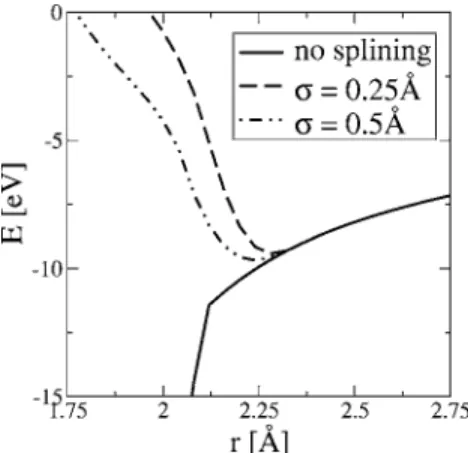
Figure 2 illustrates the collapse problem for the Ti dimer and how short-range splining stabilizes the model for small distances. As the distance between the two atoms decreases, a bonding state with an artificially low energy decreases the dimer energy. The precipitous drop in the energy of this bonding state is due to an increase in the overlap; at 1.92 Å, the overlap matrix becomes nonpositive definite, and the eigenproblem is no longer solvable. A ␴ value of 0.5 or 0.25 Å makes the dimer stable; this is necessary but not suf-ficient to solve the collapse problem for all cases.

Our parametrization has 74 parameters to be optimized, plus 3 fixed parameters. The cut-off function fc共r兲 has two fixed parametersR0andl0, while the minimum distanceRmin is set by the database. There are ten Hamiltonian and ten overlap functions, each with 3 parameters for a total of 60 parameters. The three on-site energy functions have four pa-rameters each, and a single parameter␭for the density gives 13 parameters. Finally, the short-range spline range param-eter ␴ is determined using the dimer, and testing with mo-lecular dynamic calculations and defect relaxations.13

B. Fitting database

We compile a database of electronic structure calculations of several crystal structures using full-potential linearized augmented plane wave 共FLAPW兲 calculations14 _{with the}

WIEN97program suite.15_{We use the generalized gradient} ap-proximation 共GGA兲 for the exchange-correlation energy.16 The sphere radius isRMT= 2.0 bohr= 1.06 Å; there is a neg-ligible charge leakage of 10−8_{electrons. The plane-wave} cut-offKmaxis given byRMTKmax= 9; this corresponds to an en-ergy cut off of 275 eV. The enen-ergy cut off is not as large as required in a typical pseudopotential calculation because the FIG. 1. Interpolated intersite function with short-range spline.

The parametrized function h共r兲 grows exponentially as r ap-proaches zero, though the function is only sampled in the fitting database down toR_min. Atr=R_min, we replace the function with a quartic spline that matches the value, first, and second derivatives at R_min; the dashed curve shows the growth of the original function. The spline smoothly goes to a constant value in a width of␴. Only one adjustable parameter␴is added to the entire fitting database, as

␴is the same for all functions.

FIG. 2. Energy of Ti dimer calculated with tight binding using short-range splining. Without any short-range splining, the overlap matrix becomes artificially large, creating a bonding state with very low energy at small distances; at 1.92 Å, the tight-binding dimer Hamiltonian problem becomes unsolvable. As described in the text, by short-range splining of the Hamiltonian and overlap functions, the model is stable and becomes repulsive at small distances.

plane waves are only used in the interstitial regions away from atom centers. The charge density is expanded in a Fou-rier series; the largest magnitude vector in the expansion

Gmaxis 18 bohr−1共34 Å−1兲. Local orbitals are used for thes,

p, andd solutions inside the spheres.14 _{Our core} configura-tion is Mg with semicore 3pstates represented by the localp

orbitals; our 4s, 3d, and 4p states are the valence orbitals. A Fermi-Dirac smearing of 20 mRyd共272 meV兲is used to cal-culate the total energy.17

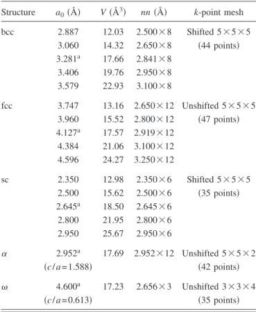
Table I shows a summary of the fitting database; it con-sists of the total energies and eigenvalues on a k-point grid for several crystal structures. Five structures are used: simple cubic 共sc兲, body-centered cubic 共bcc兲, face-centered cubic

共fcc兲, hexagonal closed-packed 共␣兲, and omega 共␻兲. The

three cubic structures are calculated over a range of volumes, while the hexagonal structures are calculated only at FLAPW equilibrium volumes andc/aratios. For each struc-ture, we fit to the total FLAPW energy of the structure and electron eigenvalues shifted by a constant on ak-point grid. The FLAPW electron eigenvalues for each structure are shifted by a constant amount so that the sum of occupied levels equals the total energy; fitting the shifted eigenvalues

will allow our model to reproduce the correct relative elec-tron energies and total energies without a pair potential. We calculate the nine lowest bands per atom above the semicore 3p states; these represent the 4s, 3d, and 4p states both be-low and above the Fermi level. We use the be-lowest six bands at eachkpoint for fitting the cubic structures, nine bands for ␣, and 12 bands for␻.

In addition to eigenvalues on a regular grid, we include eigenvalues at high symmetry points and directions in the Brillouin zone to aid in fitting.20,21_{For the three cubic} struc-tures, we calculate the eigenvalues at several high-symmetry points and directions共10 for bcc and sc, and 12 for fcc兲and then decompose the electronic wave functions in terms of the symmetry character of the eigenvalues.22_{Again, we use the} lowest six states for the high-symmetry points. We are care-ful not to fit too many eigenvalues at high-symmetry points, since the lowest nine bands in the GGA band structure may not correspond to those predicted in ourspdbasis.23

Because our fit includes the electron eigenvalues, we ex-pect our model to reproduce both total energies and energy derivatives. Phonons and elastic constants can be written in terms of the forces on atoms due to small displacements; the Hellman-Feynman theorem relates the force on an atomRito the eigenvalues as Fi= − 2

兺

␧n⬍EF

冓

␺n

冏

⳵Hˆ ⳵Ri

冏

␺n

冔

.

Thus, the electron eigenvalues of the bulk crystal contain information about phonons and elastic constants.

C. Optimization of parameters

The parameters are optimized to minimize the mean squared error. We use the nonlinear least-squares minimiza-tion method of Levenberg-Marquardt with a numerical Jacobian.24We weight eachkpoint by unity, and the result-ing total energy by 200; accordresult-ingly the total energies are weighted approximately the same as the k-point data. We initialize our parameters using the Hamiltonian and overlap values for Ti from Ref. 20 adapted to our functional form. We then fit only the environment-dependent on-site terms to the band structure of the cubic elements. After an initial fit is found, we include the hopping terms in the optimization. We proceed using only the cubic band structure, then the cubic band structure and total energies, and finally all structures and energies. After a new minimum is found, we check each function to see if the minimization has made the exponential term g_共ll⬘m_兲 too large; this corresponds to making the entire function approximately zero over the sampled range of r

values. We remedy this by resetting the e, f, and g param-eters to 0, 0, and 0.5. Several fitting runs are performed until the entire fit set is accurately reproduced.

III. RESULTS

A. Parameters and fitting residuals

Table II lists the parameters of the optimized tight-binding model. Figure 3 shows the hopping integrals h_共ll⬘m_兲共r兲 and TABLE I. Crystal structures used in tight-binding fitting

data-base. Five different crystal structures are used, with five volumes for each of the cubic crystal structures. The lattice constant a0, volume per atom, and nearest neighbor distance and multiplicity for each structure is listed. The equilibrium lattice constant for each structure is denoted bya_{. The same k-point mesh is used for all} volumes of a given structure, and is constructed using the prescrip-tion of Refs. 18 and 19. The smallest distance to appear in this fitting database isR_min= 2.350 Å.

Structure a0共Å兲 V共Å3兲 nn共Å兲 k-point mesh

bcc 2.887 12.03 2.500⫻8 Shifted 5⫻5⫻5 3.060 14.32 2.650⫻8 共44 points兲 3.281a _{17.66 2.841⫻8} 3.406 19.76 2.950⫻8 3.579 22.93 3.100⫻8 fcc 3.747 13.16 2.650⫻12 Unshifted 5⫻5⫻5 3.960 15.52 2.800⫻12 共47 points兲 4.127a _{17.57 2.919⫻12} 4.384 21.06 3.100⫻12 4.596 24.27 3.250⫻12 sc 2.350 12.98 2.350⫻6 Shifted 5⫻5⫻5 2.500 15.62 2.500⫻6 共35 points兲 2.645a 18.50 2.645⫻6 2.800 21.95 2.800⫻6 2.950 25.67 2.950⫻6 ␣ 2.952a _{17.69 2.952⫻12 Unshifted 5⫻5⫻2} 共c/a= 1.588兲 共42 points兲 ␻ 4.600a _{17.23 2.656⫻3 Unshifted 3⫻3⫻4} 共c/a= 0.613兲 共35 points兲

s_共ll⬘m兲共r兲 for a range of volumes; theRminin the database is 2.35 Å, and we interpolate each function to a constant value belowR_min. Finally, Fig. 4 shows the environment-dependent onsite energies as a function of volume for an hcp crystal withc/a= 1.588.

To use the potential for phase-transformation studies, ␴ was determined by testing the stability of共1兲the dimer,共2兲 molecular dynamics runs, and共3兲 defect relaxations. While the lowest energy pathways studied by Ref. 3 have distances of the closest approach of 2.6 Å, there were possible pathways where atoms approached within 2.3 Å of each

other. Without short-range splining, calculations of energies of structures with distances below our Rmin value can become problematic. Initially, a ␴ value of 0.529 Å was chosen based on the dimer; however, defect relaxation TABLE II. Tight-binding parametrization for titanium. The

on-site parameters are given for thes,p, anddorbitals. Each term is density dependent; the parameter in the density dependence is␭. The cutoff function has fixed parametersR₀andl₀. Next, the inter-site Hamiltonian and overlap elements are given for each of the ten symmetrized共ll⬘m兲combinations. BelowRmin, each intersite func-tion is smoothly interpolated to a constant value over the range␴.

al共eV兲 bl共eV兲 cl共eV兲 dl共eV兲 s: −3.272⫻100 _3.714⫻102 _8.029⫻103 _7.879⫻104 p: 4.974⫻100 _3.747⫻101 _{−1.874⫻10}3 _2.721⫻104 d: 3.632⫻10−1 _3.238⫻101 _8.877⫻101 _9.355⫻102 ⑀l,i=al+bl␳i 2/3 +cl␳i 4/3 +dl␳i 2 _共 2兲 ␳i=

兺

j⫽i exp共−␭2rij兲fc共rij兲: ␭2=共0.3620 Å兲−1 共3兲 fc共r兲=

冋

1 + exp

冉

r−R₀ l₀

冊

册

−1 : R0= 6.615 Å l0= 0.2646 Å 共 4兲 e_共ll⬘m兲 f_共ll⬘m兲 1 /g_共2_ll⬘m兲共Å兲 ss␴: h= −1.086⫻102eV −3.900⫻103eV/ Å 0.3277 s= 9.277 −2.624 Å−1 0.8357 sp␴: h= −1.793⫻103_{eV 8.066⫻10}2_{eV/ Å 0.4926} s= −11.81 0.02523 Å−1 _0.5993 pp␴: h= −4.865⫻102_{eV 1.816⫻10}2_{eV/ Å 0.6929} s= 0.08093 −1.351 Å−1 _1.036 pp␲: h= 1.202⫻101_{eV −8.252⫻10}0_{eV/ Å 0.8925} s= 4.478 −0.2899 Å−1 _0.8026 sd␴: h= −5.537⫻102_{eV 3.096⫻10}2_{eV/ Å 0.4772} s= −4.331 −5.085 Å−1 _0.4498 pd␴: h= −2.338⫻102_{eV 9.994⫻10}1_{eV/ Å 0.6321} s= 0.02557 −3.383 Å−1 _0.5728 pd␲: h= −4.979⫻100_{eV 7.855⫻10}−1_{eV/ Å 1.617} s= 0.1943 2.308 Å−1 _0.5882 dd␴: h= 1.706⫻102eV −1.150⫻102eV/ Å 0.5266 s= −0.9905 0.7605 Å−1 0.7990 dd␲: h= 9.920⫻100eV 3.538⫻101eV/ Å 0.5366 s= −1.490 −1.498 Å−1 0.5213 dd␦: h= 1.109⫻103eV −6.205⫻102eV/ Å 0.3340 s= 15.58 −5.276 Å−1 0.4412 兵h,s其_共ll⬘m兲共r兲=共e共ll⬘m兲+f共ll⬘m兲r兲exp共−g共ll⬘m兲 2 r兲fc共r兲 共5兲 Rmin= 2.350 Å , ␴= 0.265 Å 共6兲

FIG. 3. Tight-binding intersite Hamiltonian and overlap func-tions. The parametrized hopping integrals are shown for distances from 2.4 to 3.5 Å. TheR_minin the fit is 2.35 Å; below this, these functions are smoothly interpolated to a constant value. Circles rep-resent ␴ integrals, squares ␲ integrals, and triangles ␦ integrals; black is fors, dark gray forp, and light gray ford.

FIG. 4. Tight-binding onsite energy terms for hcp structure. The onsite energies are environment dependent in our model; we show the variation with respect to the volume of an hcp crystal with c/a= 1.588. The low volume of 10 Å3 _{has a lattice constant of} 2.44 Å, and the high volume of 25 Å3 _{has a lattice constant of} 3.31 Å. The equilibrium hcp volume is 17.56 Å3_.

calculations showed that a value of 0.265 Å was necessary to ensure stability for some of the point defects.

Table III lists the errors in our tight-binding model with respect to the fitting database. Our average total energy er-rors are approximately 1 meV; root-mean square erer-rors in thek-point energies are approximately 100 meV. The tight-binding parametrization adequately reproduces the database energetics. To test transferability, we compare to properties outside of this database; nearly all of the following results are for structures not included in the fit database.

B. Total energies

Figure 5 shows the tight-binding total energy as a function of volume for␣ and␻. These curves were not included in the fitting database; only the two points indicated. We repro-duce both the slightly lower energy of␻over␣predicted by

pseudopotential methods3_{and FLAPW calculations, as well} as the slightly lower equilibrium volume of ␻. The three cubic structures were included in the fit and have errors on the order of 3 meV/ atom共c.f., Table III兲. This shows a wide range of applicability for our model under pressure.

C. Elastic constants and phonons

Table IV shows the equilibrium lattice constants and elas-tic constants for␣, ␻, and bcc for our tight-binding model. TABLE III. Fitting errors in total energy andkpoints for

tight-binding model. For each structure, we report the absolute error in the total energy共first line兲and the rms error in allk-point energies in the fit set共second line兲. The total energy errors are on the order of 1 meV, while the rms band-structure errors are on the order of 100 meV. Low volume 共meV兲 Equilibrium 共meV兲 High volume 共meV兲 bcc 1.64 0.957 4.31 200 104 110 fcc −1.79 1.25 −0.821 136 87.1 114 sc −0.0190 −0.115 −1.60 435 195 140 ␣ −1.66 69.1 ␻ −0.00993 67.9

TABLE IV. Lattice parameters and elastic constants in units of GPa for␣,␻, and bcc Ti from tight binding, GGA, and experiment. GGA corresponds to the elastic constants found usingVASP共Refs. 25 and 26兲. The experimental␣ elastic constants are measured at 4 K共Ref. 31兲, and the bcc elastic constants at 1238 K 共Ref. 32兲. Our tight-binding model reproduces the GGA elastic constant com-binations that preserve the symmetry of the structure 共e.g., C₁₁ +C12兲, but has larger error with those that break it共e.g.,C44兲. The deviation between the bcc experimental elastic constants and our calculations is due to the high temperature needed to stabilize the bcc structure in Ti. a共Å兲 c共Å兲 C11 C12 C13 C33 C44 Tight binding ␣ 2.94 4.71 155 91 79 173 65 ␻ 4.58 2.84 184 90 52 261 100 bcc 3.27 — 87 112 — — 31 GGA ␣ 2.95 4.68 172 82 75 190 45 ␻ 4.59 2.84 194 81 54 245 54 bcc 3.26 — 95 110 — — 42 Experiment ␣ 2.95 4.68 176 87 68 191 51 bcc 3.31 — 134 110 — — 36

FIG. 5.共Color online兲Comparison of tight-binding energy as a function of volume for␣and␻with first principles data. The two filled points were included in the fit; the lines are FLAPW total energies. Our tight-binding model reproduces the fit data—slightly lower ground-state energy and equilibrium volume for␻—and the equation of state of the full-potential calculations.

FIG. 6. Comparison of tight-binding phonons for the␣ phase with experimental phonon data. The crosses are the experimental phonon frequencies at 295 K 共Ref. 34兲. The deviation from the experimental values at smallqcorresponds to the mismatch in the␣ elastic constants. Our tight-binding model does well for the high-energy optical and acoustic branches which are important for mod-eling the␣→␻transformation.

The GGA numbers correspond to the elastic constants found usingVASP.25,26_{Elastic constant combinations which do not} break symmetry such asC₁₁+C₁₂,C₁₃,C₃₃in the hexagonal crystals, and C11+ 2C12 in bcc are reproduced within ap-proximately 10%. However, the symmetry breaking elastic constant combinations such asC11−C12 andC44have larger errors. It is worth noting that none of this data, except for the bulk modulus of bcc, appears in any form in the fitting da-tabase; the agreement is a consequence of reproducing the electron eigenvalues.

We calculate phonons using the direct-force method.27–30 We calculate the forces on all atoms in a supercell where one atom at the origin is displaced by a small amount. The nu-merical derivative of the forces with respect to the displace-ment distance approximates the force constants folded with

the translational symmetry of the supercells. The Fourier transform of the force constants gives the dynamical matrix, and its eigenvalues give the phonon frequencies.33_Forq vec-tors commensurate with the supercell, the phonon frequen-cies are exact; for incommensurateq vectors, the calculated phonons are a Fourier interpolation between exact values. Our supercells are 4⫻4⫻3 for ␣, 3⫻3⫻4 for ␻, and 4 ⫻4⫻4 simple cubic cell for bcc; in all cases, a 2⫻2⫻2

k-point mesh is used in the supercell. Again, none of the following data is included in the fit database.

Figures 6–8 are the predicted phonon dispersions for our tight-binding model共TB兲, calculated at the equilibrium vol-umes for each structure. The ␣ phonons match the experi-mental values well for the high energy optical and acoustic branches; these are important for modeling the shuffle during martensitic transformation. The deviation from experiment for smallqcorresponds to our mismatch in elastic constants. The largest deviation occurs with a single low branch at the K point. The ␻ phonons are expectedly stiffer along the c

axis than in the basal plane due to the lowc/aratio. The bcc phonons show phonon instabilities corresponding to the bcc→␻ transformation 共L-2

Ⲑ

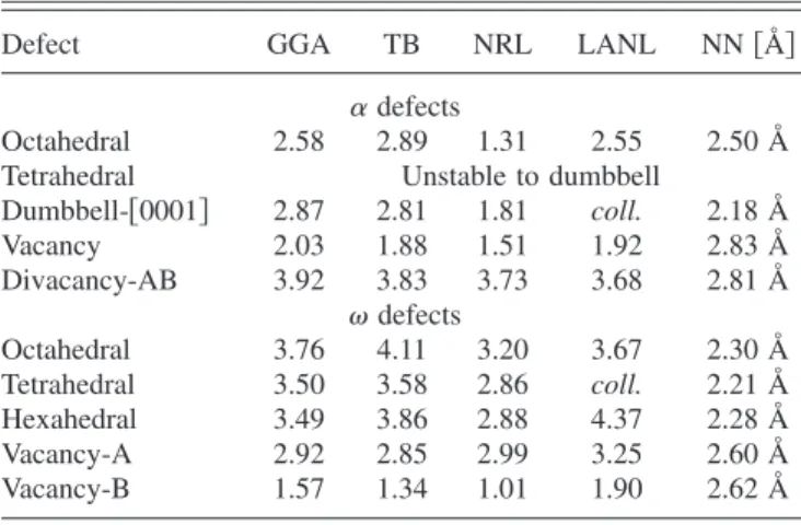
3关111兴 phonon兲 and the bcc

→␣ transformation 共T-关011兴 branch兲.35 _{The stability of the} 关0␰␰兴 direction near ⌫ is an artifact of the direct-force method in both共TB兲and GGA; the true spectra has a single imaginary branch for small ␰ values. Using an 8⫻8⫻8 simple-cubic bcc supercell in TB to derive the force con-stants removes the artificial stability; such a cell is prohibi-tively large to compute with GGA, but is expected to pro-duce the correct behavior near ⌫ as well. Throughout the TABLE V. Point defect energies in electron volts for␣and␻Ti from tight binding for different parametrizations. GGA refers to the defect formation energies calculated with VASP; TB to the param-etrization in this work; NRL to the paramparam-etrization by Mehl and Papaconstantopoulos;5and LANL to the parametrization by Rudin et al.6_{NN refers to the distance of closest approach for two atoms} in each defect in TB. The formation energies are calculated after relaxation. The defects marked coll. fell victim to the “collapse problem” during relaxation. The ␣-tetrahedral site is unstable in both TB and GGA, relaxing to form a dumbbell along the关0001兴 direction. The␻-hexahedral site is very close to the ␻-tetrahedral site 共Ref. 37兲. Many of the interstitial defects sample small dis-tances, requiring the use of short-range splining to stabilize the defects.

Defect GGA TB NRL LANL NN关Å兴

␣defects

Octahedral 2.58 2.89 1.31 2.55 2.50 Å

Tetrahedral Unstable to dumbbell

Dumbbell-关0001兴 2.87 2.81 1.81 coll. 2.18 Å Vacancy 2.03 1.88 1.51 1.92 2.83 Å Divacancy-AB 3.92 3.83 3.73 3.68 2.81 Å ␻defects Octahedral 3.76 4.11 3.20 3.67 2.30 Å Tetrahedral 3.50 3.58 2.86 coll. 2.21 Å Hexahedral 3.49 3.86 2.88 4.37 2.28 Å Vacancy-A 2.92 2.85 2.99 3.25 2.60 Å Vacancy-B 1.57 1.34 1.01 1.90 2.62 Å

FIG. 7. Predicted␻ phonons from tight binding. As expected from thec/aratio of 0.620, the phonon modes are stiffer along the

关00␰兴direction than the basal plane directions关␰00兴and关0␰0兴.

FIG. 8. Comparison of tight-binding bcc phonons with calcu-lated spectra using GGA. AtT= 0, the bcc phase in Ti is unstable, as shown by the imaginary phonon frequencies. The agreement be-tween the phonons calculated using the current model and those with GGA is good, for both stable and unstable phonons. The de-viation at thePpoint indicates too much stiffness in the TB model for motion of关111兴chains in bcc compared to GGA. The dip in the

关␰␰␰兴branch is near the L-2

Ⲑ

3关111兴phonon, which corresponds to the bcc→␻transformation pathway. The imaginary phonon for

T-关011兴corresponds to the bcc→␣ transformation mechanism共Ref. 35兲.

Brillouin zone, the TB phonons agree well with the GGA phonons. The stability of the P phonon in TB indicates too much stiffness for the motion of关111兴 chains in bcc; how-ever, the phonons in bcc are stabilized at high temperatures

共⬃1200 K兲 by strong anharmonicity.36 _{The importance of}

this deviation will need to be investigated for high tempera-ture martensitic transformations from bcc.

D. Point defects

Table V shows the formation energies of point defects for ␣ and ␻ at the equilibrium volumes for our tight-binding model. All␣calculations are performed with a 4⫻4⫻3共96 atom兲supercell and all␻with a 3⫻3⫻4共108 atom兲 super-cell, using the original lattice constants for both TB and GGA. The atoms were relaxed at fixed volume to forces of less than 5 meV/ Å, and the reference␣and␻energies were computed using the same supercell and k-point meshes 共2 ⫻2⫻2 in the supercell, 20 meV smearing兲. No point defect information is included in the initial fit; we reproduce the GGA formation energies for all of the point defects consid-ered. This indicates that our tight-binding model is appli-cable to the study of the ␣→␻ transformation path, where atoms move out of their equilibrium configurations and often close to one another.

The formation energies of point defects shows some im-provement of our model over two existing models.5,6 _The potential by Rudinet al.uses the same functional forms as our potential without short-range splining for hopping and overlap functions; Mehl and Papaconstantopoulos use the same onsite function form, but adds additional quadratic pa-rameters to the hopping and overlap functions in Eq.共5兲. All three potentials use the same on-site functional forms. For all three potentials, the binding energies versus volume, elastic constants, and phonons are similar, though Rudin’s more ac-curately captures the low frequency ␣ phonons. However, point defect formation energies compare better with GGA using our tight-binding parametrization, showing an agree-ment of 13% in formation energy for a variety of defects.

The short distances sampled by the point defects empha-size the need for short-range splining of both the overlap and

Hamiltonian functions. The collapse of two defects in the Rudinet al.model is due to the growth of the overlap ma-trices; the lower energies predicted by Mehl and Papacon-stantopoulus could be due to overly large overlap elements at short distances as well. Interstitial defects, like phase trans-formation pathways, can sample interatomic distances smaller than the smallest distance included in the fitting da-tabase; without short-range splining, this can lead to artifi-cially lower energies, or even collapse. Without short-range splining, all three tight-binding parametrizations fail for the Ti dimer at small distances: 1.92 Å for this work, 1.76 Å for Mehl and Papaconstantopoulos, and 1.28 Å for Rudinet al.

The use of short-range splines provides a solution to the collapse problem for non-orthogonal tight-binding models.

IV. CONCLUSION

We present an accurate and transferable tight-binding model with parameters determined by density-functional cal-culations. It reproduces density-functional structural energies with pressure, elastic constants, phonons, and point defect energies. The efficiency compared to GGA allows access to larger length- and time-scales with a small sacrifice in accu-racy. By fixing the short-range behavior of the potential, point defects can be accurately computed, which allows the calculation of energy barriers for phase transformation path-ways. The wide range of applicability makes it particularly well suited to the study of martensitic phase transformations, such as ␣→␻.3 Short-range splines represent a solution to the potential collapse problem of non-orthogonal tight-binding models allowing an increase in the range of applica-bility, without reoptimizing existing parameters.

ACKNOWLEDGMENTS

D.R.T. thanks Los Alamos National Laboratory for its hospitality and acknowledges support from the Ohio State University. This research is supported by DOE Grant Nos. DE-FG02-99ER45795 共OSU兲 and W-7405-ENG-36 共LANL兲. Computational resources were provided by the Ohio Supercomputing Center and NERSC.

1_{Titanium and Titanium Alloys: Fundamentals and Applications,} edited by C. Leyens and M. Peters, 共Wiley-VCH, Weinheim, 2003兲.

2_{S. K. Sikka, Y. K. Vohra, and R. Chidambaram, Prog. Mater. Sci.} 27, 245共1982兲.

3_{D. R. Trinkle, R. G. Hennig, S. G. Srinivasan, D. M. Hatch, M. D.} Jones, H. T. Stokes, R. C. Albers, and J. W. Wilkins, Phys. Rev. Lett. 91, 025701共2003兲.

4_{D. R. Trinkle, D. M. Hatch, H. T. Stokes, R. G. Hennig, and R. C.} Albers, Phys. Rev. B 72, 014105共2005兲.

5_{M. J. Mehl and D. A. Papaconstantopoulos, Europhys. Lett. 60,} 248共2002兲.

6_{S. P. Rudin, M. D. Jones, and R. C. Albers, Phys. Rev. B 69,} 094117共2004兲.

7_{W. Kohn and L. J. Sham, Phys. Rev. 140, A1133共1965兲.} 8_{J. C. Slater and G. F. Koster, Phys. Rev. 94, 1498共1954兲.} 9_{M. J. Mehl and D. A. Papaconstantopoulos, Phys. Rev. B 54,}

4519共1996兲.

10_{R. E. Cohen, M. J. Mehl, and D. A. Papaconstantopoulos, Phys.} Rev. B 50, 14694共1994兲.

11_{S. H. Yang, M. J. Mehl, and D. A. Papaconstantopoulos, Phys.} Rev. B 57, R2013共1998兲.

12_{The energy of an orbitallat atomiin the two-body} approxima-tion is具␾l,i兩Hˆ兩␾l,i典; the first three-body correction is to include hopping from atomito jand back toi.

13_{Different values of␴ could be used for each Hamiltonian and} overlap element; we use a single parameter for simplicity. 14_{D. J. Singh,Planewaves, Pseudopotentials and the LAPW Method}

共Kluwer Academic, Boston, 1994兲.

15_{P. Blaha, K. Schwart, and J. Luitz, WIEN97: A Full Potential} Linearized Augmented Plane Wave Package for Calculating Crystal Properties共Technical Universität Wien, Austria, 1999兲. 16_{J. P. Perdew, K. Burke, and M. Ernzerhof, Phys. Rev. Lett. 77,}

3865共1996兲.

17_{The large smearing was used to reduce error introduced with a} small number ofkpoints; Ref. 21 used smaller smearings with-out adverse effects.

18_{D. J. Chadi and M. L. Cohen, Phys. Rev. B 8, 5747共1973兲.} 19_{H. J. Monkhorst and J. D. Pack, Phys. Rev. B 13, 5188共1976兲.} 20_{D. A. Papaconstantopoulos,Handbook of the Band Structure of}

Elemental Solids共Plenum, New York, 1986兲.

21_{M. D. Jones and R. C. Albers, Phys. Rev. B 66, 134105共2002兲.} 22_{J. F. Cornwell, Group Theory and Electronic Energy Bands in}

Solids共North-Holland, Amsterdam, 1969兲. 23_{For example, in a bcc lattice the⌫}

25states are lower in energy than the⌫15states; however, the⌫25state corresponds to the f orbitalsx共y2_−z2_{兲 etc., while the⌫}

15states correspond top or-bitals x, y, z. Hence, we only fit the lowest 6 states at ⌫ to exclude the⌫₂₅states from the fit.

24_{D. W. Marquardt, J. Soc. Ind. Appl. Math. 11, 431共1963兲.}

25_{G. Kresse and J. Hafner, Phys. Rev. B 47, R558共1993兲.} 26_{G. Kresse and J. Furthmüller, Phys. Rev. B 54, 11169共1996兲.} 27_{K. Kunc and R. M. Martin, Phys. Rev. Lett. 48, 406共1982兲.} 28_{S. Wei and M. Y. Chou, Phys. Rev. Lett. 69, 2799共1992兲.} 29_{W. Frank, C. Elsässer, and M. Fähnle, Phys. Rev. Lett. 74, 1791}

共1995兲.

30_{K. Parlinski, Z.-Q. Li, and Y. Kawazoe, Phys. Rev. Lett. 78, 4063}

共1997兲.

31_{G. Simmons and H. Wang,Single Crystal Elastic Constants and} Calculated Aggregate Properties共MIT Press, Cambridge, MA, 1971兲.

32_{W. Petry, A. Heiming, J. Trampenau, M. Alba, C. Herzig, H. R.} Schober, and G. Vogl, Phys. Rev. B 43, 10933共1991兲. 33_{N. W. Ashcroft and N. D. Mermin,Solid State Physics共Saunders}

College, Philadelphia, 1976兲.

34_{C. Stassis, D. Arch, B. N. Harmon, and N. Wakabayashi, Phys.} Rev. B 19, 181共1979兲.

35_{W. G. Burgers, Physica共Utrecht兲 1, 561共1934兲.}

36_{K. M. Ho, C. L. Fu, and B. N. Harmon, Phys. Rev. B 29, 1575}

共1984兲.

37_{R. G. Hennig, D. R. Trinkle, J. Bouchet, S. G. Srinivasan, R. C.} Albers, and J. W. Wilkins, Nat. Mater. 4, 129共2005兲.