A Bayesian Approach to Pathway Analysis by Integrating Gene–Gene Functional Directions and Microarray Data

(1)

OpenCommons@UConn

UCHC Articles - Research

University of Connecticut Health Center Research

5-1-2012

A Bayesian Approach to Pathway Analysis by

Integrating Gene–Gene Functional Directions and

Microarray Data

David W. Rowe

University of Connecticut School of Medicine and Dentistry

Yifang Zhao

University of Connecticut - Storrs

Ming-Hui Chen

Dong-Guk Shin

Lynn Kuo

Follow this and additional works at:

https://opencommons.uconn.edu/uchcres_articles

Part of the

Life Sciences Commons

, and the

Medicine and Health Sciences Commons

Recommended Citation

Rowe, David W.; Zhao, Yifang; Chen, Ming-Hui; Shin, Dong-Guk; and Kuo, Lynn, "A Bayesian Approach to Pathway Analysis by

Integrating Gene–Gene Functional Directions and Microarray Data" (2012).UCHC Articles - Research. 144.

(2)

A Bayesian Approach to Pathway Analysis by Integrating Gene–

Gene Functional Directions and Microarray Data

Yifang Zhao,

Department of Statistics, University of Connecticut, Storrs, CT 06269, USA [email protected]

Ming-Hui Chen,

Baikang Pei,

MYSM School of Medicine, Yale University, New Haven, USA [email protected]

David Rowe,

School of Dental Medicine, University of Connecticut Health Center, Farmington, CT 06030, USA [email protected]

Dong-Guk Shin,

Computer Science & Engineering, University of Connecticut, Storrs, CT 06269, USA [email protected]

Wangang Xie,

Abbott Lab, Chicago, USA [email protected]

Fang Yu, and

Department of Biostatistics, University of Nebraska Medical Center, Omaha, USA [email protected]

Lynn Kuo

Abstract

Many statistical methods have been developed to screen for differentially expressed genes associated with specific phenotypes in the microarray data. However, it remains a major challenge to synthesize the observed expression patterns with abundant biological knowledge for more complete understanding of the biological functions among genes. Various methods including clustering analysis on genes, neural network, Bayesian network and pathway analysis have been developed toward this goal. In most of these procedures, the activation and inhibition relationships among genes have hardly been utilized in the modeling steps. We propose two novel Bayesian models to integrate the microarray data with the putative pathway structures obtained from the KEGG database and the directional gene–gene interactions in the medical literature. We define the symmetric Kullback–Leibler divergence of a pathway, and use it to identify the pathway(s) most supported by the microarray data. Monte Carlo Markov Chain sampling algorithm is given for posterior computation in the hierarchical model. The proposed method is shown to select the most supported pathway in an illustrative example. Finally, we apply the methodology to a real microarray data set to understand the gene expression profile of osteoblast lineage at defined stages of differentiation. We observe that our method correctly identifies the pathways that are reported to play essential roles in modulating bone mass.

NIH Public Access

Author Manuscript

Stat Biosci

. Author manuscript; available in PMC 2013 March 09.

Published in final edited form as:

Stat Biosci. 2012 May 1; 4(1): 105–131.

NIH-PA Author Manuscript

(3)

Keywords

Bayesian belief network; Bayesian model selection; KEGG pathways; Microarray data; Prior construction; Symmetric Kullback–Leibler divergence

1 Introduction

Genome informatics was born to cope with the vast amount of data generated by the genomic studies, in particular, to support experimental projects. The challenges for post-genome informatics are on synthesis of biological knowledge from genomic information toward understanding of general principles of life. So post-genome informatics has to be coupled with systematic experiments in functional genomics. However, the coupling is in a different direction where informatics plays a dominant role in designing experiments and prediction.

High-throughput gene analysis technology such as cDNA microarray and oligonucleotide arrays has enabled parallel analysis of thousands of genes simultaneously. Numerous statistical methods have been developed to screen for differentially expressed genes, either up- or down-regulated, in these experiments. While these projects rapidly determine gene catalogs for an increasing number of organisms, functional annotation of individual genes is still largely incomplete. It would be essential to have knowledge on coregulated genes and their interactions. Consequently, various methods have been developed toward these goals. The methods include clustering analysis on genes, neural network, Bayesian network (BN), and pathway analysis. In this paper, we will focus on pathway and Bayesian network approaches.

There are multiple sources of knowledge on pathway and gene interaction. Kyoto Encyclopedia of Genes and Genomes (KEGG) database [17] was initiated by Japanese human genome program in 1995 to link genomic information with higher order functional information by computerizing current knowledge on cellular processes and by standardizing gene annotations. These databases are often called meta-data, which means data about data. KEGG consists of three databases: PATHWAY for representing higher order functions in terms of the network of interacting molecules, GENES for the collection of gene catalogs for all completely sequenced genomes and some partial genomes, and LIGAND for the

collection of chemical compounds in the cell, enzyme molecules and enzymatic reactions. A pathway is a collection of graphical diagrams of interacting molecules obtained from many years of intensive biomedical research representing the present knowledge on various cellular or physiologic functions. It is supposed to be a computer representation of the biological system, so it can be used as part of the systems biology approach.

In addition to KEGG, such databases also include gene ontology (GO) database (Gene Ontology Consortium, 2001), and BioCarta (www.biocarta.com). We are focusing on the KEGG pathway database because it contains the directional relationship (activation or inhibition) between genes that is extremely useful in the system biology approach.

Moreover, it provides a rich set of possible structures on the gene to gene relationships. The KEGG pathway can be expanded to a general pathway database to include recently

developed and published pathways.

Another valuable source of biological knowledge is the gene-to-gene activation or inhibition knowledge aggregated from past experiments or literature search. We deposit these

directional relationships among genes in a database called PrimeDB. So from this database,

NIH-PA Author Manuscript

(4)

we can search for evidence of gene-to-gene activation or inhibition measured by the number of journals reporting these interactions.

Our goal is to investigate gene to gene interactions by integrating the following three components: the structure information of putative pathways available from pathway networks, the gene relations uncovered by literature mining as in PrimeDB and the microarray gene expression data. The first two components can be obtained before the microarray experiments, so we consider them as prior information. We will describe how we could revise our prior opinion on pathway after seeing the microarray results using Bayesian methods. Moreover, we develop methods for ranking pathways in terms of their degree of agreement with the microarray data. Figure 1 provides a schematic summary of the database integration.

Current statistics methods on pathway activities are mostly in the area of gene set enrichment analysis (GSEA) where a set of regulated genes in a pathway are compared to the regulated gene set in the microarray studies to determine whether the set is particular enriched by the pathway. Curtis et al. [3] have provided a table of software, annotation, and statistical methods used in each software. In general, Gene ontology (GO), GenMapp, KEGG, and Biocarta have been used for the annotations. Efron and Tibshirani [4] and Newton et al. [23] have provided more improved methods for gene enrichment analysis. However, all these methods are restricted to counting methods where the number of regulated genes is counted in each pathway. They have not incorporated the putative information on activation and inhibition relationships given in the KEGG database and PrimeDB.

There are also several Bayesian papers studying pathways or networks. Friedman et al. [7] propose an adaptive iterative search algorithm for an optimal Bayesian network (BN) while search is restricted to the most promising candidate parents of each gene based on some local statistics (such as correlation). Their learning algorithm uses no prior biological knowledge nor constraints. Hartemink et al. [10] extend the BN by adding edge annotation, which allows representation of additional information about the dependence relationships among genes. Sachs et al. [24] outline modeling the cell signaling pathways using BN. Sebastiani et al. [25] show the application of BN to the analysis of various types of genomic data including genomic markers and gene expression data. They also introduce the

Generalized Gamma Networks to depict the possibly nonlinear parent–child dependencies. Werhli and Husmeier [29] use Bayesian networks to reconstruct gene regulatory network by integrating microarray data and multiple sources of prior knowledge such as KEGG

pathways and promoter motifs. The prior probability of a network is modeled by a Gibb distribution, in which each source is encoded by a separate energy function. Shen and West [26] develop probability pathway annotation (PROPA) to match outcomes in gene

expression to multiple biological pathway gene sets from curated databases. Monni and Li [22] show how to utilize the prior genetic pathway and network information in the analysis of genomic data in order to obtain a more interpretable list of genes that are associated with the genotypes. Ellis and Wong [5] have examined computational algorithms for determining BN structures from experimental data. However, as far as we know, the activation and inhibition relationships among genes have hardly been utilized in the modeling steps of these procedures, except Ellis and Wong.

In this paper, we consider the pathways given in KEGG as possible models. Each pathway is a weighted graph that includes the activation and inhibition binary relationships. Given our microarray data, we are interested in knowing which pathway, or a set of pathways are most agreeable to our microarray experiment results. In the frame work of model selection, we are

NIH-PA Author Manuscript

(5)

essentially asking which pathway is most supported by the microarray data. Instead of the best one, we can also select a few pathways that are most supported by the data.

Our approach considers the results of microarray analysis as data. So we start with the selected regulated (significant) gene list from microarray analysis. The outcome for each selected genes is modeled as a discrete random variable taking values of 1 and 0, representing up-regulated and down-regulated, respectively. Then we consider a set of putative pathways (say 80 for example) from KEGG that needs to be studied. We first modify them slightly so each pathway can be considered as a BN with a directed acyclic graph. Then for each pathway structure in the set, we write down the local prior distribution for each node in the pathway. The hyperparameters in the prior information representing not only the propensities for a gene to have an activation or an inhibition effect on other genes, but also indicating the strength of this prior belief. They may have a big influence on the decision making of ranking pathways. So the formulations of them are guided by the PrimeDB which are being constructed by the informatics group of the authors here. We propose two possible solutions to the choice of hyperparameters: (A) Use the prior

information obtained from PrimeDB to formulate good estimates of these hyperparameters. Then we just plug in these estimates for the hyperparameters. (B) Treat these

hyperparameters as random variables to build another layer of hierarchial model sensibly guided by the PrimeDB and to achieve more robust results. We will develop both methods and examine their effects. We update these local distributions from KEGG and PrimeDB information conditioning on the data using the Bayes theorem. Then we rank the pathways by using the symmetric Kullback–Leibler divergence [19]. The most likely pathway has the smallest symmetric Kullback–Leibler divergence between the prior and the posterior distributions. We also extend our methodology to include all the genes in the microarray as data as given in Sect. 5.

This rest of this paper is organized as follows: Sect. 2 describes the simple Bayesian model which uses PrimeDB to specify prior directly, and defines the symmetric Kullback–Leibler divergence to measure pathway activities; Sect. 3 extends this divergence measure to the multilevel model, in which the second level prior governs our prior belief on the activation or inhibition effect aggregated by PrimeDB, A Markov chain Monte Carlo (MCMC) algorithm is proposed for posterior estimates computation; Sect. 4 demonstrates our method with a simple example, and Sect. 5 evaluates model performance through an osteoblast microarray study. We conclude the paper with a brief discussion in Sect. 6.

2 Simple Bayesian Model Using PrimeDB Directly

The easiest way to represent a network is to use a graph, which is a collection of vertices (nodes) and edges that connect vertices. The vertices can be genes, transcription factors, proteins, ligands, etc. All vertices need not be connected in a graph. A directed graph has one-way edges (arcs) that can represent an irreversible molecular reaction. In a weighted graph, weights (costs) are assigned to the edges, for example to distinguish between activation and inhibition in a signal transduction pathway.

We will first treat a pathway as a BN. A BN comprises two components: a directed acyclic graph (DAG) and a probability distribution. It is a graph with no path that starts and ends at the same node. The nodes in DAG depict stochastic variables. So the node can represent the outcome of a gene after a microarray experiment. The arcs in the DAG display directed dependencies among variables that are quantified by conditional probability distributions. Lack of arcs between two nodes indicates conditional independence. Heckerman [11] provides an excellent tutorial on the BN. We are highlighting the key points here.

NIH-PA Author Manuscript

(6)

Let Y = (Y1, . . . , YQ) denote the outcomes of Q nodes in a BN. A BN consists of:

1. a network structure S that encodes a set of conditional independence assertions about the variables in Y;

2. a set of local probability distributions associated with each node. In our application of BN on pathways, S comprises not only the set of conditional independence assertions among genes, but also the activation and inhibition effect among them. Note that in model derivation, we focus on the pathways in which each gene has a single parent, either activator or inhibitor. We also restrict our attention to a binary BN, where for each variable yi takes on only two values, with yi = 1, 0 for representing gene i

being up- or down-regulated, respectively. In Sect. 5, we demonstrate that our model is readily extended to pathways which consist of equivalently expressed genes and/or genes with multiple parents.

2.1 Notations and Transition Probabilities

We classify a gene in a pathway into three categories: (1) with no parents, (2) with an activator parent, and (3) with an inhibitor parent. In particular, we have the following notations for the three categories:

: the index set of genes without parents.

: the index set of genes with Activator parents in a pathway of Q genes.

: the index set of genes with Inhibitor parents in a pathway of Q genes.

We use to denote the probability of gene i being up-regulated, for . Given we assume a gene can be either up- or down-regulated, so a Bernoulli distribution with probability

suffices to model this outcome. We use to describe the set of initial states of a pathway, that is, for the gene(s) without parents.

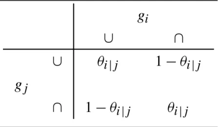
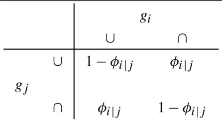
For genes with parents, we need to define their transition probabilities. Let Y_i denote the outcome for g_i with its parent to be g_j. Use symbols ∪ for being up-regulated, and ∩ being down-regulated. Then we define the transition probabilities for the connected genes as in Tables 1 and 2. That is: If g_j activates g_i, then we assume

. Consequently,

. If g_j inhibits g_i, then we assume . Consequently,

. Observe that θi|j represents an activation effect

and ϕi|j an inhibition effect from gene j to i. So the transition probabilities define the local

distribution of each node (gene) in the pathway, which is a collection of Bernoulli

distributions. Observe if we let ϕi|j = 1 – θi|j, then can collapse Tables 1 and 2 into one table.

NIH-PA Author Manuscript

(7)

Let be the parameter vector of pathway S, where is the vector of up-regulated genes with no parents, and and are the vectors of transition probabilities for genes being activated and inhibited, respectively. Let D denote the data, which are assumed to be a random sample from the joint distribution of Y. So D consists of (1) n, the total number of microarray experiments being analyzed, (2) n̄i,

the count for being up-regulated in n experiments for each , and (3) n_i|j denotes the number of concordant pairs (( ) or ( )) for gene j and gene i ordered pair in n experiments where gene j is a parent, and gene . If gene , then n_ij denotes the number of discordant pairs (( ) or ( )) for the gene j and gene i pair. By the local Markov property of the BN which says that each node is independent of its non-descendants given the parent nodes, the likelihood function, L(θs|D), of a given pathway S is the product

of the local distributions over all the genes in it. It is given as

2.2 Prior Elicitation and the Posterior Distributions

Suppose in the PrimeDB, there are ai|j journal articles citing that gj activates gi and bi|j

journal articles citing gj inhibits gi. To incorporate these prior information, we would first

assume Simple Bayesian model using PrimeDB directly. We assume θi|j ~ βe(ai|j, bi|j) for the

activation effect, and ϕi|j ~ βe(bi|j, ai|j) for the inhibition effect. If PrimeDB does not provide

information on the initial state, we can use a vague prior for it, for example, . Assuming that the parameters are mutually independent over i, the joint prior distribution can be written as:

(2.1)

Assuming there are no missing data, i.e., for each node in the BN we observe some data, the posterior distribution π(θs|D, S) is then given as:

(2.2)

So it is obtained by updating the local posterior distributions of θi|j or ϕi|j. Suppose that

KEGG suggests that gj activates gi, we need to update θi|j given the data. So we count the

number (denoted by ni|j) of ordered pairs with outcomes to be ∪ to ∪ or ∩ to ∩ from gj to gi.

It is actually the number of concordant pairs for the of (gj, gi). The number of discordant

pairs with ∪ to ∩ or ∩ to ∪ is n – ni|j . So the distribution of θi|j given data is updated to

βe(ai|j + ni|j, bi|j + n – ni|j). Similarly, if KEGG suggests that gj inhibits gi, the posterior

distribution of ϕi|j given data is βe(bi|j + ni|j, ai|j + n – ni|j).

NIH-PA Author Manuscript

(8)

2.3 Selection Criterion of Supported Pathways: Symmetric Kullback–Leibler Divergence

We propose to use the symmetric Kullback–Leibler divergence [19] to select the best pathway. The smaller symmetric Kullback–Leibler divergence between the prior and posterior distributions of a given pathway, the more supported by the data this pathway is. The Kullback–Leibler (KL) divergence is conventionally used to measure the difference between two densities. The KL divergence of the probability distribution f₁(y) from f₂(y) is defined as

We highlight the key properties of KL divergence as follows. First, the KL divergence is not a distance because it is asymmetric, i.e., KL(f₁, f₂) ≠ KL(f₂, f₁), and it does not satisfy the triangle inequality. Second, using Jensen's inequality, it can be shown that the KL divergence is nonnegative if f₂ is a proper density, and equals zero if and only if f₁ = f₂. Third, the KL divergence measures how much information f₂ carries about f₁, if f₁ is considered the “true” distribution of the data.

For more intuitive interpretation, we adopt the definition of the symmetric KL divergence introduced by Kullback and Leibler (1951)

Let us first define the symmetric KL divergence of gene i in the simple model as:

(2.3)

where

and p(y_i|pa_i, γ_i, S) is the local probability distribution for gene i, and pa_i denotes the configuration of its parent. Note that in our single-parent pathways, it can be an empty set or a singleton set having parent gene j. Equation (2.3) is an immediate consequence of the fact that π(γi|S) is a proper prior and its normalized constant is 1.

Because different pathways have different gene sizes, we use the geometric mean of the symmetric KL divergence for individual genes to correct for different dimensions. We thus define the symmetric KL divergence of a pathway S with Q genes as

(2.4)

Let π*(θs|S) be the kernel density of the prior, and let C0(S) and CD(S) be the normalizing

constants of prior and posterior distributions, respectively. We can write

NIH-PA Author Manuscript

(9)

and

Then (2.4) becomes

(2.5)

after canceling out ln(CD(S)/C0(S)) and ln(C0(S)/CD(S)) in the evaluation. This makes the

definition of the symmetric KL divergence more attractive, because the computation of CD(S)/C0(S) can be very expensive.

By local Markov property of BN, the likelihood function, L(θ_s|D), is the product of the local probability distributions. Moreover, as shown in (2.1) and (2.2), the prior distribution of pathway S can also be decomposed into the product of local prior distributions of its component genes, so can be the joint posterior distribution. Consequently, we have

Here θ_s(–_γ_i) denotes the transition probability vector of pathway S without gene i's transition probability γi. Note

Hence, the symmetric KL divergence of a pathway is the average of the symmetric KL divergences of its component genes. This has sensible interpretation. When a pathway is supported by the microarray data, we expect that, on average, the discrepancy between the local conditional distributions of its genes and their prior distributions will be small. And so will be the discrepancy between the local conditional distributions and the posterior distributions, because the prior is part of the posterior.

Since the log likelihood breaks into the sum of three parts: the one of log local distributions of initial states, of activated genes and of inhibited genes, we have

where

NIH-PA Author Manuscript

(10)

and . To evaluate the I1, I2 and I3, we will make use of the following result.

Proposition 1 If Z ~ βe(α, β), and a, b > 0, then

where ψ(α) is the standard digamma function defined as

It is straightforward to verify the proposition by interchanging the order of integration (with respect to z) and differentiation (with respect to α, β, or α + β). Consequently, we have

(2.6)

(2.7)

I₃ is similar to I₂ except ai|j is replaced by bi|j, and vice versa.

Hence, in the simple model, the computation of SKL(S) boils down to evaluating the sum of a series of the difference of digamma functions, weighted by the gene size of the pathway. Our average Q value attempts to adjust for the size of the pathways. In spite of the fact that larger pathways would be less sensitive to a few extreme SKL scores on the gene level, it is not necessary that the Q score always gives advantage to larger pathways.

3 Extension of the Symmetric KL Divergence to the Multilevel Model

3.1 Multilevel Model Guided by PrimeDB

An extra level of hierarchical Bayesian model can be constructed to allow information sharing among the same types of gene, one for activation, the other for inhibition. We define the first level prior distribution: for all i and j, θi|j|θ ~ βe(ai|j θ, bi|jθ), they are independent

over all i and j given θ. Similarly, ϕi|j|ϕ ~ βe(bi|jϕ, ai|jϕ) and are independent given ϕ. The

second level prior is independent of with known μ and ν, where denotes an exponential distribution with mean μ. By the way, it is possible to allow unknown μ and ν, so we can build a third level to allow sharing between the types of gene.

NIH-PA Author Manuscript

(11)

For the time being, we are only considering two levels with μ and ν known. Note the first level specification yields E(θi|j|θ) = ai|j/(ai|j + bi|j). This is the same mean as in the Simple

Bayesian model. However Var(θi|j|θ) = ai|jbi|j/[(ai|j + bi|j)2(ai|jθ + bi|jθ + 1)]. So this

hierarchical model adds one more parameter θ that controls our prior belief of the PrimeDB. The bigger the θ, the stronger the belief on the PrimeDB. Note that when μ = ν = 1, the distributions of transition probabilities conditional on θ and ϕ are the same as in the simple model. All genes with an activation effect suggested by KEGG share a common factor θ that can be learned from the data and PrimeDB. Similar considerations apply to the inhibition parameters.

3.2 Symmetric KL Divergence for Multilevel Model

We first extend the definitions of SKL(π(γi|S), π(γi|D, S)) and SKL(S) in the multilevel

model. Including the hyperparameters that govern our belief on the activation or inhibition effect from PrimeDB, the parameter vector of pathway S becomes . Let

Then the definition of SKL for gene i given in (2.3) sustains. Explicitly, for activated genes

D, S).

To generalize the definition of SKL(S) to the multilevel model, it is easy to see that we need to modify (2.5) to

(3.1)

Following the same logic in deriving SKL(S) in the simple model, we can verify that in the multilevel model,

Now, the joint prior distribution can be collapsed as

(3.2)

(3.3)

where (3.2) follows the facts that does not depend on θ or ϕ, is independent of ϕ, ϕs|ϕ

is independent of θ, θ and ϕ are independent. Both the assumptions of θi|j|θ being

NIH-PA Author Manuscript

(12)

independent over i and j for , and ϕi|j|ϕ being independent over i and j for , yield

(3.3).

Similarly, Ithe joint posterior distribution can be collapsed as

Substituting the specific forms of log likelihood function, the collapsed prior and posterior distributions into (3.1), we can rewrite SKL(S) as a sum of symmetric KL divergence for the genes without parents, activated, and inhibited:

(3.4) where (3.5) (3.6) with (3.7) (3.8) (3.9) and (3.10)

Equations (3.7)–(3.10) are direct results of Proposition 1. It is easy to observe that I₁′ equals to I1 that is given in the simple model, because does not depend on θ or ϕ.

NIH-PA Author Manuscript

(13)

Next, we derive the optimal form for numerically evaluating

Notice that

(3.11)

where c* is the normalizing constant for , the prior is a proper density, and,

Now we can write

and plug it into (3.11), it follows that

(3.12)

where

(3.13)

So the first term of I₂′ in (3.5) can be expressed as

Likewise, the first term of I₃′ in (3.6) can be written as

NIH-PA Author Manuscript

(14)

Therefore, when we use Monte Carlo methods to numerically evaluate the integrals in I₂′ and I₃′, we sample from the prior distribution only, rather than sample from both prior and posterior distribution of θ and ϕ. This greatly improves the efficiency of computing KL divergence.

We now summarize the algorithm for calculating the symmetric KL divergence in the multilevel model:

1. Draw θ(t) from , and draw independently ϕ(t) from , for t = 1, . . ., N.

2. I2′ is approximated by

and I₃′ is approximated by

where , , , and are given in (3.7), (3.8), (3.9), and (3.10), and

3. I1′ can be directly calculated as

4.

.

Remark It is natural to generate two Monte Carlo (MC) samples from π(θ|S) to approximate for , so that one sample is used for computing

, while the other for . However, we generate only one MC sample from π(θ|S) to compute ri1. Chen et al. [2] pointed out that the use of two MC

samples in obtaining the MC estimate of ri1 may not necessarily be more efficient than the

use of just one MC sample. They showed that the latter actually reduces the asymptotic variance of the estimate.

NIH-PA Author Manuscript

(15)

3.3 MCMC Algorithm for Sampling from the Posterior Distributions

To update the unknown parameters, we first know that the probabilities of initial states, ( ), do not depend on the hyperparameters θ and ϕ, so their posterior distributions are

βe(1 + n̄i, 1 + n – n̄i). Then we will employ Metropolis [21] within Gibbs sampling

algorithm to update the transition probabilities and hyperparameters ( ). Chen et al. [1] provide more details on the algorithm. Using the collapsing technique in drawing the Gibbs sampler proposed by Liu [20],

The last step results from conditional independence. Therefore, given the hyperparameters θ and ϕ and data, we update the transition probabilities ( ) among genes by sampling from the beta distributions. From (3.12) and (3.13), we know that π(θ|D, S) is proportional to h1(θ)μe–μθ, and π(ϕ|D, S) is proportional to h2(ϕ)νe–νϕ, and they are independent. We use

the Metropolis–Hastings algorithm to sample from π(θ|D, S) and π(ϕ|D, S). The MCMC algorithm to sample the posterior distribution can be implemented as follows:

Step 1. Generate θ and ϕ independently given the data using the Metropolis algorithm having the following target densities:

and

Since θ > 0, the local Metropolis algorithm in this step is done by sampling ξ = log(θ) instead of θ using the following steps:

1.1 Obtain the conditional density function π(ξ|D, S) by the transformation from

π(θ|D, S).

1.2

Obtain the proposal distribution , where maximizes the logarithm of

π(ξ|D, S) for ξ, and is minus the second derivative of the logarithm of π(ξ| D, S) with respect to ξ valuated at .

1.3 Let θ0 be the current value of θ. Then ξ has a current value ξ0 log(θ0).

1.4

Generate a proposal value ξ from the proposal distribution .

1.5

Update ξ from ξ0 to ξ1 with probability , where φ is the

probability density function of a standard normal variate.

1.6 Calculate θ1 = exp(ξ1).

NIH-PA Author Manuscript

(16)

Similarly, we can sample ϕ independently through the above steps 1.1–1.6 by defining ζ = log(ϕ) and using π(ϕ|D, S).

Step 2. Given the current values of θ, ϕ and data, update the transition probabilities:

and

In step 1.2, we use the optimization program optim in the R stats package. The optimization method is an implementation of the conjugate gradients method based on that by Fletcher and Reeves [6]. It will also return a numerically differentiated Hessian matrix (second derivative for a univariate case) as requested. For convergence diagnostics, we use the R coda package. The Geweke [8] method is applied here. It is based on a test for equality of the means of the first and last part of the samples from the Markov chain. If the samples are drawn from the stationary distribution of the chain, the two means are expected to be equal and Geweke's statistics has an asymptotically standard normal distribution.

4 Examples

Suppose we have the following three pathways S1, S2 and S3 suggested by KEGG. We

overlay the information collected by PrimeDB on the pathway structure. For example, we use the (7, 3) plotted on top of the right arrow between g1 and g2 to represent there are 7

journal articles having reported that g1 activates g2 and 3 articles say the contrary, g1 inhibits

g2. The KEGG information is given in the structures and weighted graphs as shown. So the

right arrows and T (stop) arrows in the graph are suggested by KEGG. For example, in all the pathways, KEGG suggests that g1 activates g2 as pictured here with the right arrow.

However, we only believe it with a certain degree. So we incorporate the possibility that g1

may actually inhibit g2 with a probability which may be small. So this framework would be

consistent with the PrimeDB results. We summarize the prior information from both KEGG and PrimeDB as follows:

1. Pathway 1 (S1):

2. Pathway 2 (S₂):

3. Pathway 3 (S₃):

NIH-PA Author Manuscript

(17)

Let us first consider the simple Bayesian model. Note the prior distribution for S₁ can be described by the product of the following five distributions: θ1 ~ βe(1, 1), θ2|1 ~ βe(7, 3),

θ3|2 ~ βe(8, 1), ϕ4|1 ~ βe(3, 3) and ϕ5|4 ~ βe(9, 6). Note the PrimeDB for the g4 to g5 reaction

says (6, 9) indicating 6 journal articles reporting activation and 9 journal articles reporting inhibition. Given ϕ5|4 is the transition probability for g4 inhibiting g5. So we construct ϕ5|4 ~

βe(9, 6) from the PrimeDB. The prior distribution for S₂ is the product of θ1 ~ βe(1, 1), θ2|1

~ βe(7, 3), θ_3|2 ~ βe(8, 1), ϕ_4|3 ~ βe(10, 1) and ϕ_5|4 ~ βe(9, 6) Note that the parameters in the beta distribution in the latter two components are in reverser order due to the inhibition effect proposed by KEGG. Suppose we have three microarray experiments yielding the following results ( ), ( ), ( ) for g₁, . . . , g₅. Then the likelihood for the data under S₁ is

. So the posterior distribution is the joint distribution of the independent components with θ1 ~ βe(3, 2), θ2|1 ~ βe(8, 5),

θ3|2 ~ βe(10, 2), ϕ4|1 ~ βe(5, 4) and ϕ5|4 ~ βe(11, 7). And, the likelihood under S2 is similar

to S1 except is replaced by , so the posterior distribution for S2 is similar to

that of S1 except the posterior component for ϕ4|1 is replaced by ϕ4|3 ~ βe(13, 1).

On the pathway selection, we need to evaluate the symmetric KL divergence for each path. We tabulate the activation and inhibition counts (ai|j, bi|j) from PrimeDB, and the concordant

and discordant counts (ni|j, n – ni|j), from the microarray experiments in Table 3. Use the

notation SKLi|j for the symmetric KL divergence for gene i with parent j. SKLi|j can be

easily calculated using (2.6) and (2.7).

We summarize the symmetric KL divergence for the three pathways in Table 4, and conclude that S2 is best supported by the microarray experiments.

Figure 2 displays the discrepancy between the prior and posterior densities for each transition probability in these three pathways. Among the comparison of the six graphs, the prior and posterior of ϕ5|4 overlap to the largest extent. For ϕ4|3, the discrepancy mainly lies

in the tiny area underneath the peak, while the moderate difference for ϕ4|1 ranges from 0.1

to 0.8. The big piece of prior for θ3|2 protruding its posterior results in larger discrepancy

than that of θ2|1. So the order of differences shown in the figure and the ranking of SKLi|j in

Table 3 are coherent.

Now we consider the multilevel models with the same data. We first generate θ(t) and ϕ(t) independently from and , for t = 1, . . ., 100000. We then give the g-functions and h-functions in three pathways. For S1, the activated gene set is . So we have

Moreover, the inhibited gene set is , so

NIH-PA Author Manuscript

(18)

Observing the S2 differs from S1 only in the arc g4, which is inhibited by g3 rather by g1. So

in S2, we replace , , and h2(ϕ) with

S3 is a subgraph of S1 with g1 activating g2 and inhibiting g4. We use the corresponding

g-functions, and change and . In addition to let μ = 1 and ν = 1, in which case transition probabilities conditional on the hyperparameters are simply the same as those in the simple model, we vary the values of hyperparameters. The results in Table 5 show that lowering both the values of μ and ν to 0.5 and 0.25, i.e., lessening our prior belief on activation and inhibition effects indicated by the PrimeDB, will not alter the ranking of the pathways. However, if we put dramatically different weights on the activation and inhibition, the ranking may be changed. In this situation, biologists apply strong

expertise information to assign the weights.

The posterior estimates for the parameters for the simple model and the multilevel model with μ = 1 and ν = 1 are listed in Tables 6 and 7, respectively. The results show that the two sets of estimates of the transitional probabilities, one with the simple model and the other with the multilevel model, are very close. Note that in the simple model, the posterior estimates for S₃ are exactly the same as their counterparts in S₁.

5 Application to an Osteoblast Lineage Study

Osteoblast differentiation is regulated by a number of systemic hormones and local factors that induce different signaling pathways in cell within the osteoprogenitor lineage. We use four biological pathways as benchmark in the present study to test the model performance. They include the Wnt signaling pathway, bone morphogenetic protein (BMP) signaling pathway, a specified calcium signaling pathway, and adipocytokine signaling pathway. The pathway structures (i.e., the molecules involved and the interactions among the molecules) can be retrieved from literatures and public databases such as KEGG and BioCarta. Kalajzic et al. [16] report the essential roles of the first two pathways in modulating bone mass. The latter two pathways are considered to be biologically irrelevant to osteoprogenitor cell differentiation. This is pointed out by other biological studies including [9, 12–15, 18, 27, 28].

We simplified the complicated pathway structures by keeping their main trunks and pruning off most of the branches. The “stripped” versions of pathways are shown in Fig. 3.

Essentially, only key players along the signaling transduction path from the beginning (ligand) to the end (usually transcription factor) and their direct regulators are kept. We made this simplification for the following reasons. First, a few key players are usually enough to determine whether a pathway is active or not. For example, in the simplest scenario of one-experiment case, knowing the expressions levels of wnt, fzd and tcf being

NIH-PA Author Manuscript

(19)

up-regulated, a biologist is inclined to predict the Wnt signaling pathway as active, whereas the three molecules are ligand, receptor and final effecter of the pathway, respectively [16]. Superior to this judgemental call, our models not only allow synthesizing multiple

experiment outcomes but also numerically measure pathways’ activities. Second, it is not necessarily true that all molecules in a pathway will behave consistently when it is active. Some of them may have functions not exclusive to the pathway, and hence show no change or even reversed change as the pathway predicts.

We validated our models through a microarray study [16] in which the mouse cavarial cultures at day 7 and 17 underwent Affymetrix microarray analysis to understand the gene expression patterns at distinct stages of osteoprogenitor maturation. Within a primary bone cell culture, limited number of cells become mature osteoblasts and represent only a small proportion of the total cell populations. Therefore, it is never certain whether the observed gene expression changes based on a heterogenous cell mixture are associated with fully differentiated osteoblast only or with other cell populations. To overcome this problem, Kalajzic et al. utilized Col1a1 promoter-green fluorescent protein transgenic mouse lines to generate more homogeneous cell populations at the preosteoblastic stage and mature osteoblast stage. They demonstrated the importance for doing this cell separation for valid microarray interpretation. For illustration purpose, we focused on the gene intensities in sorted mature osteoblast only. They were taken from the cells with 2.3GFPpos and cells with 2.3GFPneg in the 17-day-old cultures. In this three-replicate data set, we first categorized the genes in the pathways of interest as up-regulated (∪), down-regulated (∩), or equivalently expressed (EE) if their fold changes are greater than 2, less than 1/2, or in between, respectively. If a gene has a single activator parent, we counted the number of coherence (denoted as nceq in Table 8) for the ordered pair (parent, child) with the outcomes to be ( ), ( ) or (EE, EE). If a gene has a single inhibitor parent, nceq is for the (parent, child) outcomes being ( ) ( ) or (EE, EE). If a gene has odd number of multiple parents, in each replication, we checked coherence for each individual parent related to the child as in a single-parent case, then used majority rule to decide overall being coherent or not. Here, nceq is the count for overall coherence for all replications. Likewise, if a gene has even number of multiple parents and inhibitor parents are present, we used the inhibitor outcomes only to conclude being overall coherent or not per replication. If a gene has even number of single-type parents (i.e., all activators or all inhibitors), we either used majority rule to decide overall coherence per replication in no ties case, or favored being coherent in tie case.

Given the PrimeDB is still under construction, we use the KEGG database as a proxy for the PrimeDB in this example. We queried the biological pathway information stored in KEGG database to get the prior knowledge of the pathways. Each pairwise interaction in the pathways was checked against all the pathways in KEGG database. For a gene with single activator, we counted the number of pathways a, where parent–child activation interaction exists. Parameter a is then defined as a + 0.5, the number 0.5 is added to all prior counts to avoid improper prior caused by zero counts. We also defined parameter b from the number of pathways where both parent and child exist but have no activation association between. Likewise, the activation interaction was replaced with inhibition in defining a and b for genes with single inhibitor parent. For a multiple-parent case, we defined parameter a similarly from the number of pathways where at least one of the parents has interaction pointing to the child, and parameter b from the number of pathways where at least one parent exists together with the child but have no interaction between any parent– child pair. The interaction feature between parents and child, i.e., activation or inhibition, was

determined by majority rule. All the KEGG pathway information was downloaded and stored in a relational database, such that the prior parameters can be retrieved automatically.

NIH-PA Author Manuscript

(20)

Table 8 lists the parent–child directional interaction (denoted as Dtype), the prior

parameters, number of coherence, and individual SKL score per child (skl.g) based on the simple model for the four signaling pathways. Dtype takes value of 1, 0 and 2 to stand for activation, inhibition and multiple-parent case, respectively. Table 9 gives the SKL scores for the four pathways based on the simple model and multilevel model. The two signaling pathways that play essential role in the osteoblast lineage progression, Wnt and BMP, have smaller SKL scores than the other two pathways. In multilevel models 1–3, we set the values of the hyperparameters that govern our belief on the prior counts acquired from KEGG, at all equal to 1, 2 or 0.5. The ranking of the pathways is not sensitive to the choice values of hyperparameters.

It is worthwhile noting that the above extension to multiple parents does not seem to follow along the line of a Bayesian network. It is possible to have the usual Bayesian network extension to construct conditional distribution given multiple parental nodes. However, lack of prior information from the literature search in practice has made us resolve to a more realistic approach, as presented here.

6 Discussion

We have proposed a novel methodology to integrate the high-throughput data, pathway structure and medical literature regarding the gene-gene directional interactions (PrimeDB). We construct BN from a pathway database, and use PrimeDB to guide the choices of prior parameters or hyperparameters in the BN. Then we show how to update these information using high-throughput genomics experiments. Our method numerically measures the strength of agreement between each pathway and the experiment using the symmetric Kullback Leibler measure incorporating the activation/inhibition association permeated in the biomedical literature. So we can rank the importance of these pathways in terms of their relatedness to the biological experiments to gain further knowledge in system biology. When a pathway agrees with the experimental data structurally, we would expect the pathway has a small SKL divergence measure. However, this cannot be guaranteed if the prior belief is terrible. So our method also relies on good choices of the prior distribution that should be flat and has huge support. In the illustration using real data, we have chosen the KEGG pathway database as the primary source of pathway structure and its gene-gene interaction as representative of medical journal counts (PrimeDB). The result might rely on the extant knowledge from a single data repository. However, our methodology is general enough that can be applied to any good databases that include gene-gene direction relationships as a substitute of the PrimeDB.

When a pathway is identified, it suggests the pathway is most agreeable with the data presented. On the other hand, the pathway with the highest K–L divergence suggests the pathway structure is not well supported by the data. This may be caused by (1) unexpected data, (2) dubious pathway structure, or both. So it has potential to provide more insights into the pathways.

We have used small sample size in our simulated and real examples, primarily small sample size is common in microarray experiments. Nevertheless, our method can handle any sample size as well. Microarray techniques are known to be noisy for biologists, so their results are often questioned by the biologists. Small sample exacerbates this situation. So incorporating a Bayesian frame work and borrowing information from the literature will add credibility to the microarray studies. Moreover, the multilevel model provides a more robust framework for sharing information among similar genes in evaluating the pathways.

NIH-PA Author Manuscript

(21)

Our method can handle large networks quite efficiently. It first computes the SKL score for each gene independently, then takes their averages as the pathway SKL score. In the simple model, the gene-specific SKL score reduces to a linear function of digamma functions. It hence can readily handle large pathways at fast speed. For the multilevel model, we use a collapsing technique and as a result sample from the prior distribution only instead of from both prior and posterior distributions of θ and ϕ, the two parameters that govern prior belief of the literature count. This greatly improves the efficiency in the numerical evaluation of the integrals in I₂′ and I₃′, the sums of the SKL scores for activated genes and inhibited genes. R programs have been developed based on this method. In the osteoblast lineage study, the four pathways have 11, 12, 9 and 10 genes, respectively. It takes less than 13 seconds in total to compute their SKL scores of the multilevel model using R 2.13.0 on a laptop computer with 2nd generation Intel Core i5-2410M processor 2.30 GHz. So it should not be a burden to compute SKL for large pathways which consist of about a hundred nodes at most as shown in KEGG.

Starting with the gene expression data from microarray, we first applied some statistical tests to classify the genes as up-regulated, down-regulated, or equivalently expressed. Fold change was used in our real data analysis. Then we construct Bayesian network for each pathway. So our study applies to the continuous gene expressions. However, we simplify the agreement assessment by discretizing the data. It would be interesting to extend our method to directly using the continuous gene expression. Nevertheless, we do not think the

extension will be straightforward especially on a realistic prior construction.

We think the strength of this paper is on its ability to handle directed graphs with directed prior information on gene functions. On the other hand, our method can be modified to handle undirected graphs. In that, we will not differentiate activation or inhibition direction, change all of them into connection, then our method with reduced parameters can handle the undirected graph. For mixed graphs with directed and undirected edges, we need to add the connected part for the direction-unknown edges, then we can handle them similarly. In this paper, we also assume that microarray outcomes are available for all the genes considered in the pathway (BN). However, it is often in practice so, that the pathway includes genes that microarray may not explore. So this falls into the missing data problem in BN. Conditional inference with incomplete data and model selection can still be carried out using Expectation and Maximization (EM) algorithm or MCMC. Further investigation on this issue should be worthwhile.

Acknowledgments

The work of Yifang Zhao, Baikang Pei, David Rowe, Dong-Guk Shin, Wangang Xie, Fang Yu, and Lynn Kuo was partially supported by Grants NIH/NIGMS P20GM65764, NIH/NIDCR U24DE016495, and State of Connecticut Stem Cell Initiative 06SCC04. Ming-Hui Chen's work was partially supported by NIH grants GM70335 and CA74015.

References

1. Chen, M-H.; Shao, Q-M.; Ibrahim, JG. Monte Carlo methods in Bayesian computation. Springer; New York: 2000.

2. Chen M-H, Huang L, Ibrahim JG, Kim S. Bayesian variable selection and computation for generalized linear models with conjugate priors. Bayesian Anal. 2008; 3:585–614. [PubMed: 19436774]

3. Curtis RK, Oresic M, Vidal-Puig A. Pathways to the analysis of microarray data. Trends Biotechnol. 2005; 23(8):429–435. [PubMed: 15950303]

4. Efron B, Tibshirani R. On testing the significance of sets of genes. Ann Appl Stat. 2007; 1:107–129.

NIH-PA Author Manuscript

(22)

5. Ellis B, Wong WH. Learning causal Bayesian network structures from experimental data. J Am Stat Assoc. 2008; 103:778–789.

6. Fletcher R, Reeves CM. Function minimization by conjugate gradients. Comput J. 1964; 7:148–154. 7. Friedman N, Linial M, Nachman I, Pe'er D. Using Bayesian networks to analyze expression data. J

Comput Biol. 2000; 7(3-4):601–620. [PubMed: 11108481]

8. Geweke, J. Evaluating the accuracy of sampling-based approaches to calculating posterior moments.. In: Bernado, JM.; Berger, JO.; Dawid, AP.; Smith, AFM., editors. Bayesian statistics 4. Clarendon; Oxford: 1992.

9. Hartmann C. A Wnt canon orchestrating osteoblastogenesis. Trends Cell Biol. 2006; 16(3):151–158. [PubMed: 16466918]

10. Hartemink A, Gifford DK, Jaakkola TS, Young RA. Bayesian methods for elucidating genetic regulatory networks. IEEE Intell Syst Biol. 2002; 17(2):37–43.

11. Heckerman, D. A tutorial on learning Bayesian networks.. 1995. Technical Report MSR-TR-95-06, Microsoft Research

12. Hoffmann A, Gross G. BMP signaling pathways in cartilage and bone formation. Crit Rev Eucar Gene Expr. 2001; 11(1-3):23–46.

13. Ishii M, Kurachi Y. Muscarinic acetylcholine receptors. Curr Pharm Des. 2006; 12(28):3573–3581. [PubMed: 17073660]

14. Jensen ED, Gopalakrishnan R, Westendorf JJ. Regulation of gene expression in osteoblasts. BioFactors. 2010; 36(1):25–32. [PubMed: 20087883]

15. Jimia E, Hirataa S, Shina M, Yamazakia M, Fukushimaa H. Molecular mechanisms of BMP-induced bone formation: Cross-talk between BMP and NF-?B signaling pathways in osteoblastogenesis. Jpn Dent Sci Rev. 2010; 46(1):33–42.

16. Kalajzic I, Staale A, Yang W-P, Wu Y, Johnson SE, Feyen JHM, Krueger W, Maye P, Yu F, Zhao Y, Kuo L, Gupta RR, Achenie LEK, Wang H-W, Shin D-G, Rowe DW. Expression profile of osteoblast lineage at defined stages of differentiation. J Biol Chem. 2005; 280:24618–24626. [PubMed: 15834136]

17. Kanehisa M, Goto S. KEGG: Kyoto encyclopedia of genes and genomes. Nucleic Acids Res. 2000; 28(1):27–30. [PubMed: 10592173]

18. Kay GG, Abou-Donia MB, Messer WS, Murphy DG, Tsao JW, Ouslander JG. Antimuscarinic drugs for overactive bladder and their potential effects on cognitive function in older patients. J Am Geriatr Soc. 2005; 53(12):2195–2201. [PubMed: 16398909]

19. Kullback S, Leibler RA. On information and sufficiency. Ann Math Stat. 1951; 22(1):79–86. 20. Liu JS. The collapsed Gibbs sampler with applications to a gene regulation problem. J Am Stat

Assoc. 1994; 89:958–966.

21. Metropolis N, Rosenbluth AW, Rosenbluth MN, Teller AH, Teller E. Equation of state calculations by fast computing machines. J Chem Phys. 1953; 21:1087–1092.

22. Monni, S.; Li, H. Bayesian methods for network-structures genomic data.. In: Chen, MH.; Dey, DK.; Muller, P.; Sun, D.; Ye, K., editors. Frontiers of statistical decision making and Bayesian analysis: In honor of James O. Berger. Springer; New York: 2010. p. 303-315.

23. Newton M, Quintana F, Den Boon J, Sengupta S, Ahlquist P. Random-set methods identify distinct aspects of the enrichment signal in gene-set analysis. Ann Appl Stat. 2007; 1:85–106.

24. Sachs K, Gifford D, Jaakkola T, Sorger P, Lauffenburger DA. Bayesian network approach to cell signaling pathway modeling. Sci Signal Transduct Knowl Environ. 2002; 148:e38.

25. Sebastiani, P.; Abad, M.; Ramoni, M. Bayesian networks for genomic analysis.. In: Dougherty, ER.; Shmulevich, I.; Chen, J.; Wang, ZJ., editors. Genomic signal processing and statistics. Hindawi Publishing Corporation; New York: 2004. p. 281-320.

26. Shen, H.; West, M. Bayesian modeling for biological annotation of gene expression pathway signatures.. In: Chen, MH.; Dey, DK.; Muller, P.; Sun, D.; Ye, K., editors. Frontiers of statistical decision making and Bayesian analysis: In honor of James O. Berger. Springer; New York: 2010. p. 285-302.

27. Tilg H, Moschen AR. Adipocytokines: mediators linking adipose tissue, inflammation and immunity. Nat Rev Immunol. 2006; 6:772–783. [PubMed: 16998510]

NIH-PA Author Manuscript

(23)

28. van Amerongen R, Nusse R. Towards an integrated view of Wnt signaling in development. Development. 2009; 136(19):3205–3214. [PubMed: 19736321]

29. Werhli A, Husmeier D. Reconstructing gene regulatory networks with Bayesian network by combining expression data with multiple sources of prior knowledge. Stat Appl Genet Mol Biol. 2007; 6(1):1–45.

NIH-PA Author Manuscript

(24)

Fig. 1.

Flowgram of data sets integration

NIH-PA Author Manuscript

(25)

Fig. 2.

Prior and posterior densities for transition probabilities

NIH-PA Author Manuscript

(26)

Fig. 3.

Four simplified signaling pathways

NIH-PA Author Manuscript

(27)

NIH-PA Author Manuscript

Table 1

(28)

NIH-PA Author Manuscript

Table 2

(29)

NIH-PA Author Manuscript

Table 3

Summary of the directional counts and SKL per gene Genes

ai bi n ̄i n – n ̄i SKL i g1 1 1 2 1 2 ψ (2) + ψ (1) – 3 ψ (5) + 5 = 0.75 Genes ai| j bi| j ni| j n – n i| j SKL i| j g2|1 7 3 1 2 ψ (8) – ψ (7) + 2[ ψ (5) – ψ (3)] – 3[ ψ (13) – ψ (10)] = 0.4868 g3|2 8 1 2 1 2[ ψ (10) – ψ (8)] + ψ (2) – ψ (1) – 3[ ψ (12) – ψ (9)] = 0.5662 g4|1 3 3 2 1 ψ (4) – ψ (3) + 2[ ψ (5) – ψ (3)] – 3[ ψ (9) – ψ (6)] = 0.1964 g5|4 6 9 2 1 ψ (7) – ψ (6) + 2[ ψ (11) – ψ (9)] – 3[ ψ (18) – ψ (15)] = 0.0249 g4|3 1 10 3 0 3[ ψ (13) – ψ (10)] – 3[ ψ (14) – ψ (11)] = 0.0692

(30)

NIH-PA Author Manuscript

Table 4

Pathway selection based on the simple model

Pathway SKL(S)

S 1 ⅕(SKL1 + SKL2|1 + SKL3|2 + SKL4|1 + SKL5|4) = 0.4049

S 2 ⅕(SKL1 + SKL2|1 + SKL3|2 + SKL4|3 + SKL5|4) = 0.3794

(31)

NIH-PA Author Manuscript

Table 5

SKL

(S

) based on the multilevel model

Pathways μ = 1 μ = 0.5 μ = 0.5 μ = 1 μ = 0.25 μ = 1 μ = 0.25 ν = 1 ν = 0.5 ν = 1 ν = 0.5 ν = 0.25 ν = 0.25 ν = 1 S1 0.7194 0.5090 0.5608 0.6680 0.3694 0.6330 0.4540 S2 0.6285 0.4535 0.4700 0.6131 0.3376 0.6009 0.3636 S3 0.7216 0.5539 0.6225 0.6524 0.4388 0.6070 0.5521

(32)

NIH-PA Author Manuscript

Table 6

Posterior estimates based on the simple model S

1 S2 Param. Mean Std. Error Param. Mean Std. Error θ2|1 0.6154 0.1300 θ2|1 0.6154 0.1300 θ3|2 0.8333 0.1034 θ3|2 0.8333 0.1034 ϕ4|1 0.5556 0.1571 ϕ4|3 0.9286 0.0665 ϕ5|4 0.6111 0.1118 ϕ5|4 0.6111 0.1118

(33)

NIH-PA Author Manuscript

Table 7

Posterior estimates based on the multilevel model S

1 S2 S3 Param. Mean Std. Error Param. Mean Std. Error Param. Mean Std. Error θ 1.2642 1.0880 θ 1.2457 1.1083 θ 1.0593 1.0273 ϕ 1.2905 1.0494 ϕ 1.1019 1.0084 ϕ 0.9984 0.9873 θ2|1 0.5922 0.1549 θ2|1 0.5948 0.1578 θ2|1 0.5653 0.1768 θ3|2 0.8260 0.1194 θ3|2 0.8217 0.1217 ϕ4|1 0.5653 0.1676 ϕ4|3 0.9381 0.0668 ϕ4|1 0.5752 0.1766 ϕ5|4 0.6159 0.1245 ϕ5|4 0.6141 0.1358

(34)

NIH-PA Author Manuscript

Table 8

Prior counts and individual SKL scores for the four pathways Pathway

Parent a Child a Dtype b nceq a b skl.g Wnt Wnt5a Fzd1 1 3 4.5 0.5 0.145 Dkk1 Lrp6 0 2 1.5 0.5 0.883 FL c Dvl2 2 1 3.5 2.5 0.354 Dvl2 Gsk3b 0 3 4.5 1.5 0.370 GAAC c Ctnnb1 2 3 5.5 4.5 0.584 Ctnnb1 Tcf7 1 1 8.5 1.5 1.428 Bmp Bmp8a Amhr2 1 3 1.5 0.5 0.807 AS c Smad1 2 2 1.5 0.5 0.883 Smad1 Smad4 1 2 1.5 0.5 0.883 ST c Smad2 2 3 1.5 4.5 2.754 Smad2 E2f4 1 3 1.5 0.5 0.807 E2f4 Myc 1 1 1.5 0.5 2.750 Smad2 Sp1 1 2 1.5 0.5 0.883 SM c Cdkn2b 2 1 1.5 2.5 0.188 Tgfb1 Tgfbr1 1 2 7.5 0.5 1.494 Calcium Htr5a Gnas 1 3 1.5 0.5 0.807 Gnas Adcy8 1 3 4.5 1.5 0.370 Adcy8 Prkacb 1 3 5.5 1.5 0.270 Prkacb Pln 0 0 1.5 0.5 5.950 Pln Atp2a1 0 0 1.5 0.5 5.950 Atp2a1 Calm3 1 1 1.5 1.5 0.450 Calm3 1500003O03Rik 1 2 2.5 1.5 0.188 Calm3 Camk2g 1 2 5.5 1.5 0.201 Adipocytokine Tnfrsf1b Traf2 1 1 1.5 0.5 2.750 Traf2 Mtor 1 2 1.5 1.5 0.450 Traf2 Mapk9 1 2 1.5 2.5 0.683 Traf2 Ikbkb 1 3 1.5 4.5 2.754

(35)

NIH-PA Author Manuscript

Pathway Parent a Child a Dtype b nceq a b skl.g MMLS c Irs1 2 2 3.5 0.5 1.166 Lepr Jak2 1 1 2.5 0.5 3.383 Jak2 Stat3 1 2 2.5 0.5 1.021 Stat3 Socs3 1 3 2.5 0.5 0.374

(36)

NIH-PA Author Manuscript

Table 9

SKL(S) of the four pathways

Pathways Simple Model Multilevel Model1 Multilevel Model2 Multilevel Model3

Wnt 1.0922 1.0673 1.1565 0.9828

Bmp 1.3916 1.2471 1.4976 1.0197

Calcium 1.8263 1.7778 2.0835 1.4889