Comparison of Stochastic Volatility
Models Using Integrated Information
Criteria
A Thesis Submitted to the
College of Graduate Studies and Research
in Partial Fulfillment of the Requirements
for the degree of Master of Science
in the Department of Mathematics and Statistics
University of Saskatchewan
Saskatoon
By
Yunyang Wang
c
Permission to Use
In presenting this thesis in partial fulfilment of the requirements for a Postgraduate degree from the University of Saskatchewan, I agree that the Libraries of this University may make it freely available for inspection. I further agree that permission for copying of this thesis in any manner, in whole or in part, for scholarly purposes may be granted by the professor or professors who supervised my thesis work or, in their absence, by the Head of the Department or the Dean of the College in which my thesis work was done. It is understood that any copying or publication or use of this thesis or parts thereof for financial gain shall not be allowed without my written permission. It is also understood that due recognition shall be given to me and to the University of Saskatchewan in any scholarly use which may be made of any material in my thesis.
Requests for permission to copy or to make other use of material in this thesis in whole or part should be addressed to:
Head of the Department of Mathematics and Statistics 142 Mcclean Hall 106 Wiggins Road University of Saskatchewan Saskatoon, Saskatchewan Canada S7N 5C9
Abstract
Stochastic volatility (SV) models are a family of models that commonly used in the model-ing of stock prices. In all SV models, volatility is treated as a stochastic time series. However, SV models are still quite different from each other from the perspective of both underlying principles and parameter layouts. Therefore, selecting the most appropriate SV model for a given set of stock price data is important in making future predictions of stock market. To achieve this goal, leave-one-out cross-validation (LOOCV) methods could be used. However, LOOCV methods are computationally expensive, thus its use is very limited in practice. In our studies of SV models, we proposed two new model-selection approaches, integrated widely applicable information criterion (iWAIC) and integrated importance sampling infor-mation criterion (iIS-IC), as alternatives to approximate LOOCV results. In iWAIC and iIS-IC methods, we first calculate the expected likelihood of each observation as an integral with respect to the corresponding latent variable (the current log-volatility parameter). Since the observations are highly correlated with their corresponding latent variable, the integrated likelihood of each tth observation (yobs
t ) is expected to approximate the expect likelihood of yobs
t calculated from the model with y
obs
t as its holdout data. Second, the integrated ex-pected likelihood is used, as a replacement of the exex-pected likelihood, in the calculation of information criteria. Since the integration with respect to the latent variable largely reduces the model’s bias towards the corresponding observation, the integrated information criteria are expected to approximate LOOCV results. To evaluate the performance of iWAIC and iIS-IC, we first conducted an empirical study using simulated data sets. The results from this study show that iIS-IC method has an improved performance over the traditional IS-IC, but iWAIC does not outperform the non-integrated WAIC method. A further empirical study using real-world stock market return data was subsequently carried out. According to the model-selection results, the best model for the given data is either the SV model with two independent autoregressive processes, or the SV model with nonzero expected returns.
Acknowledgements
I thank my adviser, Dr. Longhai Li, for his kindly guidance in my thesis project and the thesis writing. I thank my committee member, Dr. Juxin Liu, for her suggestions to improve my thesis. I thank my colleague, Ms. Zhouji Zheng, for her preliminary work on the project. I also thank the University of Saskatchewan and the U of S math & stats department for providing me the financial support during my studies, and my parents for their mental support on me over the years.
Contents
Permission to Use i Abstract ii Acknowledgements iii Contents iv List of Tables viList of Figures vii
1 Introduction 1
1.1 Stochastic Volatility Models . . . 1
1.2 Review of Model Comparison Methods . . . 2
1.3 Contributions of This Thesis . . . 6
2 The Stochastic Volatility Models and the Model-Fitting Process 9 2.1 The Stochastic Volatility Models . . . 9
2.2 Bayesian Inference and Markov Chain Monte Carlo Sampling for Fitting SV Models . . . 15
3 Statistical Methods for Comparing the Stochastic Models 21 3.1 The Cross-Validation Information Criterion . . . 21
3.2 The Deviance Information Criterion . . . 23
3.3 The Widely Applicable Information Criterion . . . 24
3.4 The Importance Sampling Information Criterion . . . 26
3.5 The Integrated WAIC and IS Criteria . . . 27
4 Empirical Results 31 4.1 Simulation Studies . . . 31
4.2 An Empirical Study on S&P 100 Data . . . 41
5 Conclusions and Discussions 47 References 51 Appendix A THE DEVIATION OF THE CONDITIONAL DISTRIBU-TIONS OF LOG-VOLATILITIES IN THE AR-SV MODELS 55 A.1 Conditional Distribution of ht Given h−t in AR(1) Process . . . 55
A.2 Conditional Distribution of ht Given h−t in AR(2) Process . . . 57 A.3 Conditional Distribution of ht Given h−t in Two Independent AR(1) Processes 59
Appendix B R CODE FOR THE STOCHASTIC VOLATILITY MODELS 60
B.1 Generating Simulated Data Sets From Model 6 . . . 60
B.2 Model Specifications and Model Fittings . . . 61
Appendix C R CODE FOR CALCULATING THE INFORMATION
CRI-TERIA 80
C.1 Utility Functions . . . 80
C.1.1 Sums and Means . . . 80
C.1.2 WAIC and IS-IC . . . 81
C.1.3 Functions Related to the Calculation of the Integrals in Model 5 . . . 82
List of Tables
4.1 Average Parameter Rˆ for Simulated Data . . . 33
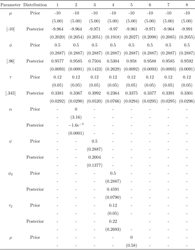
4.2 Average Parameter Estimates for Simulated Data . . . 37
4.2 Average Parameter Estimates for Simulated Data (continued) . . . 38
4.3 The Model Selection Results for Simulated Data. . . 40
4.4 The Average CPU Time Used to Compute the Criteria for the 100 Simulated Data Sets (in Seconds) . . . 41
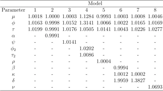
4.5 Parameter Rˆ for S&P 100 Index Data . . . 43
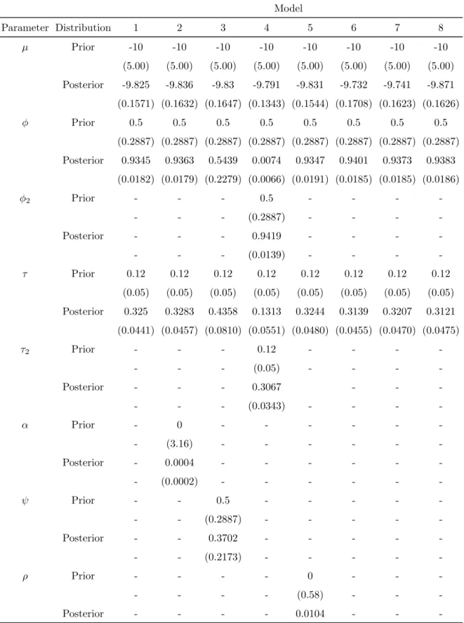
4.6 Parameter Estimates for S&P 100 Index Data . . . 44
4.6 Parameter Estimates for S&P 100 Index Data (continued) . . . 45
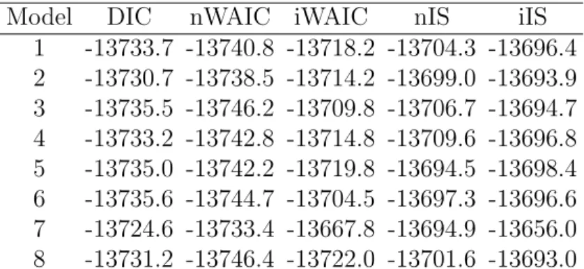
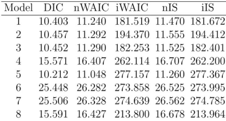
4.7 The DIC, nWAIC, iWAIC, nWAIC, nIS, and iIS for S&P 100 Index Data 46 4.8 The CPU Time Used to Compute the Criteria for S&P 100 Index Data (in Seconds) . . . 46
List of Figures
4.1 Example of trace plots of parameters in model 6 . . . 35
4.2 Example of trace plots ofφ andφ2 in model 4 when two Markov chains converge to different modes . . . 36
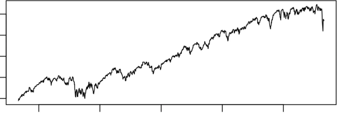
4.3 The plot of S&P 100 daily returns and index data from September 2010 to August 2015 . . . 42
Chapter 1
Introduction
1.1
Stochastic Volatility Models
Stochastic volatility (SV) models are widely used in modeling stock prices, as described in journal papers written by Taylor (1982) and Hull and White(1987). In the basic stochastic volatility model, the mean-corrected daily continuously compounded returns yt can be mod-eled as normal distributions with stochastic volatilities. Unlike the exponentially weighted moving average (EWMA) model and the generalized autoregressive conditional heteroskedas-ticity (GARCH) model, log-volatilities are treated as a Markov process in the SV model.
As a result of the Markov process, the log-volatility itself becomes a stochastic process. Therefore, SV models do not need to assume a constant volatility or a fixed volatility process like some other models (i.e., the well-known Black-Scholes model proposed by Black and Scholes(1973)). Since volatilities do change over time, the assumption of a constant volatility is a major shortcoming for many non-SV models, especially when the time horizon is long. Thus SV models are often a good alternative in the modeling of stock prices and some other derivatives with changing volatilities.
In addition to the basic model, many extended SV models are used for the purpose of stock price modeling as well, as described in the papers published by Harvey et al. (1994);
Shephard (1996); Gallant and Tauchen(1996); Chernov et al. (2003).
In this thesis, eight different models were tested and compared for stock price modeling. Each of the tested models is either the basic SV model or its variation.
To sample from the posterior distributions of SV model parameters using Markov chain Monte Carlo method, we need to know a function that is proportional to the posterior distributions. To achieve this goal, Bayesian inference were used in the study. According
to Bayes’ rule, given the prior distribution of model parameters π(θ), and a set of observed data D, the posterior distribution of model parameters is proportional to the product of the posterior likelihood function of model parameters f(D|θ)π(θ) and the prior distribution of model parameters:
fpost(θ|D) =
f(D|θ)π(θ)
R
f(D|θ)π(θ)d(θ), (1.1)
where θ are model parameters, fpost(θ|D) is the posterior distribution of model parameters, and fpost stands for posterior density functions.
1.2
Review of Model Comparison Methods
Currently, many model comparison techniques are used to select an appropriate model for a given real data set. Since the ability to make out-of-sample predictions is a vital criterion for comparing models, a proper model-comparison method should be able to choose the model that best predicts out-of-sample data.
Naturally, cross-validation methods are used to evaluate out-of-sample predictive per-formance, and one of the most commonly used cross-validation method is leave-one-out cross-validation (LOOCV). In LOOCV, each validating set contains only one observation from the original data set, and the training set comprises all the other observations. When we estimate out-of-sample predictive performance with LOOCV, we hold one observation out, and test the model with the holdout observation upon the completion of the training. This training-and-testing procedure goes on until each of the observations has served as a holdout. In the end, predictions of the holdouts are compared against true observations, and a loss function is calculated as a measure of the goodness of the prediction. However, since LOOCV requires multiple rounds of model-training procedure, the method is often very computationally expensive.
Common alternatives to cross-validation approach is to measure the adjusted within-sample predictive accuracy. Since within-within-sample predictions of a model is always better as model-complexity increases, the goodness of within-sample predictions needS to be penal-ized with a model complexity measure to estimate the out-of-sample predictive performance. Therefore, in the alternative approaches, the model selection criteria are corrected by
im-posing a penalty for the model’s complexity. As a result, comparison methods are able to select models with balanced goodness-of-fit and model complexity as an approximate of out-of-sample predictive information criterion. Examples of the adjusted within-sample pre-dictive accuracy approach include Akaike information criterion (AIC), deviance information criterion (DIC), widely applicable information criterion (WAIC), and importance sampling information criterion (IS-IC, or just IS). Formulas of these information criteria for models without latent variables (or viewing latent variables as part of parameters θ) are given as follows. We will use yobs
t to denote the actual observation of the variable yt.
• The Akaike Information Criterion and Deviance Information Criterion The Akaike information criterion (AIC) has long been used to evaluate the quality of a model for a given set of data. The goodness of fit is AIC is measured by the logarithm of the maximum likelihood function for the model, and the model complexity is measured simply by the number of parameters:
AIC =−2[log(L)−k], (1.2)
whereLis the maximal value of the likelihood function, andk is the number of param-eters in the model.
The deviance information criterion (DIC) is a widely used Bayesian model selection criterion that is closely related to the AIC. As described by Spiegelhalter et al.(2002), the general formula for DIC is given by:
DIC =−2[logf(yobs|θ)−
pD], (1.3)
where the term logf(yobs|θ) measures within-sample goodness of fit, and the term p
D is the effective number of parameters (a measure of model complexity).
The first term in the DIC formula, logf(yobs|θ), measures the relative goodness of fit
be calculated by the following formula:
θ =Epost(θ|yobs). (1.4)
On the other hand, the second term in the formula, pD, measures effective number of parameters. The pD can be calculated by the following formula:
pD = 2[logf(yobs|θ)−Epost[logf(yobs|θ)]. (1.5)
A larger pD value suggests a larger number of effective model parameters, which corre-sponds to a higher level of model complexity. As a result, thepD needs to be subtracted from the goodness-of-fit measurement in order to correct for model complexity.
The use of DIC is limited by a number of theoretical issues (Spiegelhalter et al., 2002,
2014). In the case of SV models, the number of latent variable increases with the increase of the sample size in latent variable models, causing non-regular likelihood-based statistical inference problems. As a result, the asymptotic justification of DIC is not validated, since the asymptotic theory of DIC is derived from regular likelihood (Gelman et al., 2014). Another major shortcoming of DIC is that the DIC is not invariant to re-parametrization. For the same model with different parametrizations, we may get different DIC values.
• The Widely Applicable Information Criterion
The widely applicable information criterion (WAIC) is an approximation to the cross-validation approach proposed by Watanabe (2010). In the WAIC method, goodness-of-fit is measured by calculating the summation of the log-scaled expected predictive probability density of sample points yobs
1 , ..., y obs n : n X t=1
logEpost[f(yobst |θ)], (1.6)
where θ is the estimated model parameters. In this formula, a higher log-probability summation value suggests a better fit of the data.
On the other hand, model-complexity is measured by effective number of parameters (pW AIC): pW AIC1 = 2 n X t=1
{logEpost[f(yobs
t |θ)]−Epost[logf(y obs t |θ)]}, or (1.7) pW AIC2 = n X t=1
Varpost[logf(ytobs|θ)], (1.8)
wherepW AIC1 is calculated by summing up the difference between the logarithm of the expected posterior probability of each observation and the expected value of the log-scaled posterior probability of each observation, and pW AIC2 is the sum of the variance of the posterior probability of each observation. Either one of the two can be used as an estimate of the effective number of parameters. A higher pW AIC implicates that a more complicated model is used, and the model needs to be penalized more as a result. Similar to the DIC method, the WAIC criterion takes both goodness-of-fit and model complexity into consideration:
WAIC =−2 n
X
t=1
logEpost[f(yobst |θ)] + 2pW AIC. (1.9)
In the formula above, the summation of the log-probabilities measures how well the model predicts the sample data, and effective number of parameters (pW AIC) adjusts the criterion for model complexity.
The WAIC method is different from AIC and DIC methods mainly on how posterior parameter estimates are used during the calculation. In the AIC and DIC methods, likelihood functions are calculated according to point estimates of the posterior param-eters, while in the WAIC method, the calculation is based on the posterior distribution of the parameters. Therefore, the WAIC approach generally works better on reflecting posterior uncertainties, and can be used as an alternative to the AIC and DIC methods when parameters are non-identifiable (Celeux et al., 2006). However, the asymptotic justification of WAIC only holds when all the observations are independent of each other, which is not the case in SV models.
• The Importance Sampling Information Criterion
As described by Gelfand et al. (1992) and Gelfand (1996), the importance sampling information criterion (IS-IC) approach approximates cross-validation results by intro-ducing a weight measurement:
Wt= 1 f(yobs
t |θ)
. (1.10)
The weight formula suggests that the higher the posterior predictive density of yobs
i is, the smaller the weight is. Using this weight, the IS-IC can be calculated as:
IS-IC = −2 n X t=1 log Epost[f(y obs t |θ)Wt] Epost(Wt) (1.11) = −2 n X t=1 log 1 Epost[1/f(yobs t |θ)] , (1.12)
where the IS-IC is −2 times the summation of the weighted estimates of expected pointwise predictive densities.
The IS-IC is asymptotically equivalent to LOOCV, but the criterion’s approximation to LOOCV may be negatively affected if a certain observation has a large impact on the value ofθ (for example, an outlier observation) (Peruggia,1997;Vehtari,2001; Vehtari and Lampinen,2002;Epifani et al., 2008; Li et al., 2015).
1.3
Contributions of This Thesis
In this thesis, we propose to compare stochastic volatility models which have latent vari-ables (such as ht) using regular DIC, WAIC, IS-IC methods, as well as two new approaches named integrated widely applicable information criterion (iWAIC) method and integrated importance sampling information criterion (iIS-IC, or just iIS) method. In non-integrated WAIC (nWAIC) and IS-IC (nIS-IC, or nIS) approaches, the likelihood f(yobs
t |ht,θ) is com-puted conditional on the full set of fitted model parameters and latent variablesht. However, unlike LOOCV, nWAIC and nIS are calculated according to models fitted with entire data
set. Therefore, the f(yobs
t |ht,θ) might be biased towards ytobs and thus cannot be considered as out-of-sample likelihood. In our particular case of SV models, estimated log-volatility parameters, ht, are strongly correlated with corresponding ytobs. As a result, the bias of the likelihood f(yobs
t |ht,θ) could be greatly reduced if direct uses of ht is avoided.
If we denote h−t as all the estimated log-volatilities except ht, and θ as all the other parameters, then this integrated likelihood f(yobs
t |h−t,θ) could be calculated according to the following integral:
f(yobs t |h−t,θ) = Z ∞ −∞ f(yobs t |θ, ht)f(ht|θ, h−t)dht, (1.13) where t= 1, ..., n, andn is total number of observations.
Once f(yobs
t |h−t,θ) is calculated, the integrated likelihood could be plugged into the
nWAIC and nIS formulas (in replacement of f(yobs
t |ht,θ)) to calculate the iWAIC and iIS values. In our studies, we proposed integrated iWAIC and iIS methods as potential alterna-tives to the nWAIC and nIS. Therefore, the performance of the two newly proposed model selection methods needs to be evaluated as well. In order to make comparisons, another popular approach, DIC, was also included in the testing process.
In our studies, DIC, nWAIC, nIS, iWAIC, and iIS criteria are studied for their performance in model selection. The model selection methods were used to select models that best fit the given data sets. In the first study, data sets were firstly generated from an SV model, and the generated data sets were subsequently fitted into eight candidate SV models. The data-generating model is one of the candidate models, and we choose to use eight different models so that it is unlikely that a certain model-selection criterion would favor the correct model just by chance. In the end, the models were compared by applying DIC, nWAIC, nIS, iWAIC, and iIS methods. Through this simulation study, we have found that all the tested information criteria are able to select the correct model (in this case, the data-generating model) most of the time, and the integration does improve the performance of IS method. In the second study, a real set of stock market return data (S&P 100) was respectively fitted into the eight different SV models, and DIC, nWAIC, nIS, iWAIC, and iIS criteria were used to determine the best model for the given data set. The results of the real-world stock data
indicate that the best model for the given data is either the SV model with two independent autoregressive processes of ht, or the SV model with a non-zero expected return.
Chapter 2
The Stochastic Volatility Models and the
Model-Fitting Process
2.1
The Stochastic Volatility Models
The price of a corporation stock is determined by the entity’s capability to generate future cash flows, and is also affected by the stock’s supply and demand. If we make an investment on a certain stock, then the profit of the investment on the stock over a period of time is called the stock’s rate of return. In practice, the return of a stock is closely related to the stock’s volatility. If yt is continuously compounded rate of return, then the relationship between the two can be modeled by the following formula:
yt|σt∼N(0, σt2), t= 1, ..., n, (2.1)
where σ2
t is the corresponding price volatility.
The stock price volatility is a measure of expected magnitude of the change of prices (up or down) of an underlying asset, which is a very important feature of a stock. The volatility for a given stock is essential in predicting the price of a stock itself, as well as many other stock-related derivatives. For example, according to the famous Black-Scholes model, a European call option on a given stock (with the same strike price and expiration) requires more premium (more valuable) when the implied volatilities of the underlying stock is higher (Black and Scholes, 1973). In addition, from the risk management point of view, volatilities of stocks are needed to determine the value at risk (VaR) of a portfolio (Giot and Laurent,
Traditional approaches such as historical simulation may not recognize changes in volatil-ity, and generalized autoregressive conditional heteroskedasticity (GARCH) models are often used to forecast future volatilities as a result (Engle,1982;Bollerslev,1986). For example, in the GARCH (1, 1) model, volatilities σ2
t are calculated according to the following formula: σ2t =ω+αyt2−1+βσt2−1, t= 1, ..., n, (2.2)
where ω =ρVL is weighted long-run variance (VL is long-run variance, and ρ is its weight), αyt2−1 is weighted previous period’s return (yt−1 is previous period’s return), and α is its weight), and βσ2
t−1 is weighted previous volatility estimate (β is the weight). This model becomes popular in estimating volatilities due to its simplicity and some theoretical justifi-cations. However, in practice, the estimated parameters often renders the model unusable. For example, the summation of the estimated weights assigned to yt2−1 and σ2t−1,α+β, often exceeds one. In this situation, the volatility is not a stationary process.
Stochastic volatility (SV) models are alternatives to GARCH models in the modeling of stock price volatilities (Taylor, 1982; Hull and White, 1987). In SV models, volatility is considered as a random process. By allowing randomness in the process, SV models have more theoretical benefits. In this study, we tested several autoregressive stochastic volatility (AR-SV) models, which is a popular sub-category of SV models. In basic AR-SV models, the logarithm of volatilities , ht=log(σt), are modeled as a stochastic autoregressive process:
ht =µ+φ(ht−1 −µ) +vt, t= 1, ..., n, (2.3)
which can also be written as:
ht = (1−φ)µ+φht−1+vt, t= 1, ..., n, (2.4)
where µ is long-run volatility,ht−1 is previous volatility, andvt is normally distributed with mean 0 and variance τ2. If the weight assigned to previous log-volatility is between zero and one, then ht is a stationary process. This formula also shows that the long-run mean of log-volatilities is evaluated as µ, indicating ht is mean reverting. This mean-reverting property
of ht is consistent with many empirical studies. In addition, the equation suggests that current log-volatility is dependent on the previous log-volatility estimate, which satisfies the volatility-clustering feature of stock price (high volatility is typically followed by another high volatility, and vise versa). Furthermore, the introduction of vt suggests that log-volatility is not a fixed function of its previous estimate, but also has its own randomness.
Given log-volatilities, daily stock returnsyt can be modeled as:
yt= exp ht 2 ut, t = 1, ..., n, (2.5)
where ut follows a normal distribution with mean zero and variance τ2, and is independent of vt.
In the literature, various AR-SV models have been proposed. In this study we consider the following eight plausible AR-SV models, as described and summarized by Berg et al.
(2004).
• Model 1
This model is the basic AR-SV model as we mentioned previously. The state equation governing the log-volatility process is given by:
ht =µ+φ(ht−1−µ) +vt, t= 1, ..., n, (2.6)
and the observation equation equation of daily return is:
yt= exp ht 2 ut, t = 1, ..., n, (2.7)
whereutis a standard normal distribution,vt∼N(0, τ2), andvtandutare independent of each other.
• Model 2
Model 2 is a variation of the basic SV model. In this model, the state equation of the log-volatilities is the same with the basic AR-SV model, but the mean of daily returns
yt is α (nonzero) instead of zero: ht = µ+φ(ht−1−µ) +vt, t= 1, ..., n, (2.8) yt = α+ exp ht 2 ut, t = 1, ..., n, (2.9)
whereutis a standard normal distribution,vt∼N(0, τ2), andvtandutare independent of each other. In practice, it makes sense to assume that the expected daily return is not zero. According to the “trade-off between risk and reward” principle, the more risk taken, the greater the potential reward (Lundblad,2007). Therefore, mean returns on stocks should be at least not less than the risk-free rate.
• Model 3
In this model, log-volatilities ht follow an AR(2) process:
ht = µ+φ(ht−1−µ) +ψ(ht−2−µ) +vt, t = 1, ..., n, (2.10) yt = exp ht 2 ut, t= 1, ..., n, (2.11)
whereutis a standard normal distribution,vt∼N(0, τ2), andvtandutare independent of each other.
This equation is best used to model a log-volatility process that has a lower autocorre-lation with lag-1 log-volatility. According to the Yule-Walker equation (Cheng, 2005), for any ht in this AR(2) process, lag-1 autocorrelation (the correlation betweenht and ht−1) is the coefficient ofht−1, which is φ. On the other hand, the lag-n autocorrelation (the correlation between ht and ht−n) is given by φn +ψn−1. Therefore, the model indicates that current log-volatility is less correlated with its lag-1 log-volatility, but is more correlated with all the other lagged log-volatilities.
• Model 4
(1994), Shephard (1996), andChernov et al. (2003): h(1)t = φh(1)t−1+vt(1), t= 1, ..., n, (2.12) h(2)t = φ2h (2) t−1+v (2) t , t= 1, ..., n, (2.13) yt|ht = exp µ 2 + h(1)t 2 + h(2)t 2 ! ut, t = 1, ..., n, (2.14)
where ut is a standard normal distribution, and v (1)
t ∼ N(0, τ2), v (2)
t ∼ N(0, τ2). Be-sides, v(1)t , v(2)t , and ut are all independent of each other.
In this model, the log-volatility ht is given by µ+h (1) t +h (2) t , with h (1) t and h (2) t being two independent AR(1) processes.
• Model 5
Model 5 allows a correlation between ut and vt+1, which causes an asymmetric effect of yt. This correlation betweenut and vt+1 has long been noticed by Black(1976), and
Engle and Ng (1993). In a previous study completed by Engle and Ng (1993), it was found that return shocks has an impact on volatility. As a result, it is reasonable to assume a correlation between the two. In model 5, the correlation is described by the following covariance matrix:
ut vt+1 ∼N( 0 0 , 1 ρτ ρτ τ2 ) (2.15)
Therefore, the SV model equation and the state equation of ht can be written as:
ht = µ+φ(ht−1−µ) +ρτexp(−0.5ht−1)yt−1 +τp1−ρ2w t, t= 1, ..., n, (2.16) yt|ht = exp ht 2 ut, t= 1, ..., n, (2.17)
where ut and wt are both independent normal distributions with mean 0 and unit variance.
• Model 6
In this model, a jump component (an additional random upward or downward move-ment of an observation) is included in observation equation. Besides, yt is also affected by its lagged observation yt−1:
ht = µ+φ(ht−1−µ) +vt, t= 1, ..., n, (2.18) yt = βyt−1+stqt+ exp ht 2 ut, t= 1, ..., n, (2.19)
where vt and ut are independently distributed with vt ∼ N(0, τ2) and ut ∼ N(0,1). In addition, another parameter st with the distribution of log(1 + st) ∼ N(−δ
2
2, δ 2) measures jump sizes, and qt ∼ Bern(κ) is the probability of the occurrence of jumps. The β parameter is a measurement of the sensitivity of the current observation (yt) to the previous observation (yt−1).
In general, this model suggests that the current return yt is determined by the current price volatility, the occurrence of a random jump, and the previous observation yt−1.
• Model 7
Similar to model 6, model 7 also includes a jump component, but not the previous observations: ht = µ+φ(ht−1−µ) +vt, t= 1, ..., n, (2.20) yt = stqt+ exp ht 2 ut, t= 1, ..., n. (2.21)
The distributions of all the parameters in model 7 are identical to the ones in model 6. • Model 8
To obtain this model, Gaussian observation errors in the observation equation are replaced by Student t distributions with ν degrees of freedom:
ht = µ+φ(ht−1−µ) +vt, t= 1, ..., n, (2.22) yt = exp ht 2 ut, t = 1, ..., n. (2.23)
where ut∼tν is a student t distribution withν degrees of freedom, vt ∼N(0, τ2), and vt and ut are independent of each other. This model assumes the distribution of daily return yt has a heavier tail comparing to the basic model.
Since the errors are symmetric and nonnormal, scale-mixtures of normals could be used for model fitting according to Andrews and Mallows (1974):
yt ∼ N 0,exp(ht) wt , t= 1, ..., n, wt ∼ 1 νχ 2 ν = Gamma ν 2, ν 2 , t= 1, ..., n. (2.24)
2.2
Bayesian Inference and Markov Chain Monte Carlo
Sampling for Fitting SV Models
It is rather difficult to apply classical statistical inferences, such as maximum likelihood es-timation, to SV models due to the nonanalytic form of the likelihood function. To overcome this problem, several alternative approaches have been proposed. For example, in quasi-maximum likelihood method proposed by Harvey et al. (1994), an approximation of the actual likelihood function is obtained by considering the distribution of log(yt) as a nor-mal distribution. This approximated function (quasi-maximum likelihood function) is then maximized instead of the actual likelihood function.
In another approach called efficient method of moments (EMM), the derivative of quasi-likelihood function is used as the moment condition of generalized method of moments (GMM). The EMM-estimated parameters are then calculated by minimizing the norm of the moment condition. By using this moment condition instead of selecting a few low order moments on an ad hoc basis, EMM method is found to be more efficient (Andersen et al.,
1999).
In our studies, we used Bayesian inference for SV models. According to Bayes’ rule, given the prior distributions of model parameters π(θ,h) and the observed datayobs, the posterior
distributions of model parameters can be expressed as:
fpost(θ,h|yobs) =
f(yobs|θ,h)π(θ,h)
R
f(yobs|θ,h)π(θ,h)d(θ,h), (2.25)
where f(yobs|θ,
h) is the likelihood function of model parameters (θ,h) given the observed data yobs, and the integral in the denominator calculates the normalizing constant. Since
it is usually very hard to calculate the integral, we apply MCMC sampling technique to sample from the posterior distributions of model parameters based on the numerator func-tion f(yobs|θ,
h)π(θ,h), which is proportional to the posterior density function of model parameters. This Bayesian approach, together with MCMC technique, is more efficient than non-likelihood methods in estimating parameters of SV models (Jacquier et al., 2012). A more recently developed MCMC technique, Hamiltonian Monte Carlo method, is especially suitable for SV models due to its better handling of correlated model parameters ht ( Car-penter et al., 2015).
In order to fit the models to a given data set, we used Markov chain Monte Carlo (MCMC) method to sample from the posterior distributions of parameters in each model. In an MCMC process, model parameters were sampled according to a Markov chain. The Markov chain is a random process that undergoes state transitions in a given state space. Given a finite state space, a Markov chain is bound to reach a stationary state (invariant distribution) when the chain is long enough (Gilks, 2005).
In MCMC, a Markov chain is designed to sample model parameter(s) so that the equi-librium distribution(s) of the Markov chain is the posterior distribution of the parameter(s). Several algorithms have been developed to accomplish this goal. One of the most commonly used MCMC methods is Metropolis-Hastings algorithm proposed by Metropolis et al.(1953). This algorithm starts with a non-normalized posterior probability density function f(θ|yobs
) (θis the parameter of interest), an arbitrary initial valueθ0, and an arbitrary transition prob-ability density function Q(a|b). In the first step of the Metropolis-Hastings algorithm, a new candidate θi is generated according to the probability density function of Q(θi|θi−1), where i is the iteration number. In the following step, an acceptance rate α = f(θi|yobs)Q(θi−1|θi)
f(θi−1|yobs)Q(θi|θi−1)
Finally, we need to determine whether to accept the newly-proposed θi. If α is greater than one, the θi would be automatically accepted; if α is between zero and one, the θi will be accepted with a probability of α (if rejected, set θi = θi−1). These steps will be repeated until we have collected necessary samples.
Although the Metropolis-Hastings algorithm could theoretically provide samples from a posterior distribution in almost any situation, the method might not work well in some practical problems, for example the sampling for SV models described in section 2.1. Since the posterior density ofθ does not change over the Metropolis-Hastings iterations, it is quite likely that the sampling process gets stuck in a low-density region of θ. For example, if the θi in the current iteration is far away from the high-density region, and most of the newly-proposed θi+1 happen to have a very low acceptance rate α over the current θi, then the Markov chain is highly likely to be stuck at the θi for quite a long time. If the Markov chain gets stuck in the low-density region, we may observe an extremely slow convergence of the chain. This convergence failure greatly limits the use of the Metropolis-Hastings method, especially when the number of parameter is large.
To overcome the convergence problem of the Metropolis-Hastings algorithm, the Hamil-tonian Monte Carlo (HMC) method was developed for posterior sampling (Alder and Wain-wright,1959;Andersen,1980;Neal et al.,2011). The HMC method makes use of the concept of a canonical distribution by replacing the energy function with the Hamiltonian energy function H(q,p): P(q,p) = 1 Z exp[−H(q,p)] (2.26) = 1 Z exp[−U(q)] exp[−K(p)] = Cexp[−U(q)] exp[−K(p)],
where Z and C are normalizing constants, q is the position variable corresponding to the potential energy, and p is the momentum variable that determines the kinetic energy. The application of canonical distribution is to ensure a statistical equilibrium (steady state) in the long run, since the mechanical system will reach a thermal equilibrium with a heat bath eventually. To sample from the posterior distribution of parameterq, we define the following
position function:
U(q) =−logg(q|yobs
), (2.27)
where g(q|yobs) is non-normalized posterior probability density function of f(q|yobs), which
could be easily obtained according to the Bayes rule. In our studies of the SV models, q is (θ, h1, . . . , hn)
On the other hand, the momentum variablepis used as an auxiliary variable to facilitate the sampling of our target distribution of q. If we want to sample {q1, ...,qd} from the target distribution of f(q|yobs), we would need to assignd auxiliary variables {p
1, ...,pd} as well. The pis usually defined as a zero-mean, unit variance multivariate normal distribution independent of each other and the position variable q. Therefore, the kinetic function K(p) can be expressed as:
K(p) = d X i=1 1 2p 2 i (2.28)
We are able to use the HMC method to draw sample from the posterior thanks to three fine properties of the Hamiltonian dynamics: conserved total energy, volume preservation, and time reversible. First, since the Hamiltonian dynamics is defined by the following differential equations: dqi dτ = ∂H ∂pi =pi; (2.29) dpi dτ = − ∂H ∂qi =−∂U ∂qi , (2.30)
where τ is the physical time. We can easily tell that the Hamiltonian dynamics is conserved over time: dH dτ = d X i=1 dqi dτ ∂H ∂qi + dpi dτ ∂H ∂pi = d X i=1 ∂H ∂pi ∂H ∂qi − ∂H ∂qi ∂H ∂pi = 0. (2.31)
The conserved total energy indicates the Hamiltonian function H is invariant. Therefore, when we use the Hamiltonian dynamics to propose a new state in the Metropolis updates, the acceptance rate is always one. This high acceptance is desirable in the Metropolis method. However, in practice, we are only able to approximate the Hamiltonian dynamics using
multiple steps of discrete transformation functions (e.g., the leapfrog method), which makes the actual acceptance rate a little bit smaller than one.
Besides, the Hamiltonian dynamics also preserves the volume after each transformation. According to Liouville’s theorem, the phase space is conserved under the dynamics. This volume preservation property is important, since constantly changing phase spaces can distort the sampling process.
Thirdly, the time reversible property of the Hamiltonian dynamics comes from the way the transformation (denoted by Ts) works. Since the mapping from (q(τ),p(τ)) to (q(τ + s),p(τ+s)) is one-to-one according to theTs, the backward mapping from (q(τ+s),−p(τ+ s)) to (q(τ),−p(τ)) can be achieved through T−s. This time reversible property suggests the transformation leaves the target distribution invariant. As a result, the transformation would provide a random sample from the target distribution.
One common approach of the Hamiltonian dynamics is through the application of multiple steps of leapfrog transformation. In each single leapfrog jump, we start at a given state of (p(τ),q(τ)) at timeτ, and after an arbitrary period of time , the new state (p(τ+),q(τ+ )) is calculated by the following formulas:
ˆ pi τ + 2 = pˆi(τ)− 2 ∂U ∂qi (ˆq(τ)); (2.32) ˆ qi(τ +) = qi(τˆ ) +piˆ τ + 2 ; (2.33) ˆ pi(τ +) = pˆi τ + 2 − 2 ∂U ∂qi (ˆq(τ +)). (2.34)
Since a series of leapfrog transformations is an approximation to the Hamiltonian dynamics, the energy function H is not totally invariant. To compensate for this, we would accept the newly proposed state (p0,q0) with a Metropolis acceptance rate instead of one.
Once we define the position function, the kinetic energy function and the Hamiltonian dynamics, we can start the HMC sampling process with a current state q0 by repeating a three-step iteration. In the first step of the iteration, we randomly select −p0 from their independent standard normal distributions, and then we negate the variables to get p0. In the second step, through the application ofLleapfrog steps with an arbitrary time period of each, a new (p0, q0) is proposed from the current state (p0, q0). In the end, the newly-proposed
(p0, q0) is accepted with a probability of min(1,exp[−H(q0, p0) +H(q,−p)]). If rejected, the
next state would be the same as the current state. However, no matter whether the new state is accepted or not, the momentum variable p would always be re-generated from its independent multivariate normal distribution at the beginning of each iteration.
In the HMC sampling process, the choice of the leapfrog step size parameter and the trajectory length parameter L is of paramount importance to the performance of the HMC sampling. In order to best approximate a continuous Hamiltonian dynamics process and thus avoid a high rejection rate, the step size parameter cannot be too large. However, an that’s too small might slow down the trajectory too much. The trajectory length parameter, L, on the other hand, also needs to be carefully chosen to minimize auto-correlations between different samples. In other words, the ideal choice of L should be able to maximize the the difference between q0 and q0.
In our studies, the model-fitting process was completed through the application of rstan package, which is an R package based on stan sampler (Guo et al., 2016). The stan is a recently developed MCMC sampler using the no-U-turn (NUT) HMC algorithm, which is a modified HMC method that with a default scheme for choosing L (Carpenter et al., 2015;
Gelman et al., 2015). In the NUT sampling, the trajectory will automatically stop once the next single leapfrog jump would make q0 closer to q0. Through the application of the NUT HMC algorithm, the stan sampler generally works much better than traditional samplers when dealing with models with a large number of parameters. As a result, we used the rstan package in our studies to make posterior parameter sampling for our SV models.
Chapter 3
Statistical Methods for Comparing the
Stochas-tic Models
Model selection is important in the study of stock market data and forecasting future trends. By using the correct model, the property of the data is better understood and interpreted, thus better predictions and estimations can be made. Using wrong models in practice, on the other hand, may lead to unexpected losses that could be prevented.
Traditional methods, including the mean squared error (MSE) and the coefficient of de-termination (R2), only measure the fit of the data to the models. Since adding additional parameters into a model typically increases the goodness-of-fit, these methods tend to favor complex models that may over-fit the data. To overcome the over-fitting problem, cross-validation methods are introduced. The cross-cross-validation methods involve partitioning the data set into two subsets, fitting the model with one subset, and testing the model with the other subset. Although the cross-validation methods seem to be able to fully address the over-fitting problem, these methods are time-consuming and costly. Alternatively, many methods impose penalties for model complexity.
3.1
The Cross-Validation Information Criterion
Among all cross-validation methods, leave-one-out-cross-validation (LOOCV) is usually used to minimize the number of tests to run. In addition, LOOCV makes better use of the given data set than any other cross-validation method. In LOOCV, the information criterion
(cross-validation information criterion, or CVIC) is computed by the following formula: CVIC =−2 n X t=1 logf(yobs t |y obs −t). (3.1)
In this equation, the information criterion is calculated as−2 times the sum of logf(yobs
t |y
obs −t). The bigger the CVIC value, the worse the fit.
Applied to SV models, the LOOCV posterior predictive density of the tth observation, f(yobs
t |y
obs
−t), can be calculated by the following equation: f(yobs t |y obs −t) = Z Z f(yobs t |θ, ht)f(θ,h1:n|yobs−t)dθdh1:n. (3.2) In the equation above, hj is log-volatility parameter corresponding to the jth observation (yobs
j ), andθ are all the other non-log-volatility model parameters. In addition,y
obs
−t and h−t represent all observations and latent variables exceptyobs
t and ht, respectively. The equation (3.2) calculates f(yobs
t |y
obs
−t) as the expected value of f(y
obs
t |θ, ht), where the distributions of θ and ht could be obtained according to the data set yobs−t. If we assume that the structural information of the log-volatility series (h1:n) is preserved, then MCMC samples ofθ,h1:n|yobs−t can be drawn according to the following joint posterior distribution:
f(θ,h1:n|yobs−t)∝
Y
j6=t f(yobs
j |hj,θ)f(h1:n|θ)f(θ), (3.3)
where f(yobs
j |hj,θ) is the probability density of yobsj conditional onhj and θ, f(h1:n|θ) is the probability density of h1:n conditional on θ, and f(θ) is the prior distribution of θ. Once we obtain the sample of the parameters,f(yobs
t |y
obs
−t) could be readily calculated according to equation (3.2) by approximating the integral with averaging over MCMC samples. Finally, the CVIC values of the SV models could be subsequently computed by formula (3.1) for each t = 1, . . . , T.
However, when the model fitting process is time consuming, even LOOCV method might become too expensive. In LOOCV, we need to simulate at least T Markov chains. In our study of SV models, the time for a computer to finish running a single Markov chain ranges from hours to several days, which is extremely time-consuming. Therefore, non-exhaust
cross-validation methods are sometimes used to approximate exhaustive methods to further reduce the computation. Instead of testing all possible combinations of training sets and validating sets, non-exhaustive methods only use a finite number of randomly selected combinations.
In general, cross-validation approach is effective in dealing with optimistic bias problem, but the great cost of computation limits its use. In our studies, the number of observations in each data set is big, and the model fitting process is extremely time consuming (typically from hours to days). Therefore, cross-validation approach is not a good option. Instead, sev-eral other methods (DIC, WAIC, IS) were used to approximate cross-validation information criterion.
3.2
The Deviance Information Criterion
The deviance information criterion (DIC) is often used for Bayesian model selections ( Spiegel-halter et al.,2002). In particular, DIC method is very useful in the Bayesian model selection problems when the posteriors are generated from Markov chain Monte Carlo (MCMC) sim-ulation. In the case of MCMC simulation, both expected deviance of fit (D) and effective number of parameters (pD) can be readily calculated from samples of simulated posterior pa-rameters and the original data set (Dempster,1997). For example, for the basic SV model:
ht = µ+φ(ht−1−µ) +vt, t= 1, ..., n, (3.4) yt = exp ht 2 ut, t = 1, ..., n. (3.5)
The MCMC simulation will provide us with a list of parameter and latent variable ht values from each iteration. So at the end of the simulation, we have h(i)1 , h(i)2 , ..., h(i)n , i= 1, ..., I, where imeans the ith sample and the I is the total number of samples. So in this particular case, the goodness-of-fit measurement, D, is calculated by the following formula:
D = −2Eθ|y,h[logf(y|θ, ht)], which can be estimated by (3.6)
b D = −2 n X t=1 1 I I X i=1
logf(yobs
t |h (i)
where logf(yobs
t |h (i)
t ) is the log-scaled probability density of thetthobservation with mean zero and standard deviation exp(h(i)t ). On the other hand, the measurement of model complexity, pD, is given by D−D(θ). The calculation of D has been shown in the above formula, and the following equation can be used to compute the D(θ):
d D(θ) = −2 n X t=1 logf(yobs t |ht), t= 1, ..., n, (3.8)
where ht is the posterior mean ofht, which can be estimated by the average of ht in MCMC samples.
In general, the major advantage of DIC method is that the method is very easy to im-plement and is proven to work reasonably well for the problems with identifiable parame-terization. The DIC method typically does not require many model specific adjustments, and the calculation is usually not time consuming. Therefore, DIC method is a cost-efficient solution to Bayesian model selection problems. However, the method assumes a posterior multivariate normal distribution, which may not be guaranteed in some cases.
3.3
The Widely Applicable Information Criterion
The widely applicable information criterion (WAIC, also called non-integrated WAIC, or nWAIC) is a recently developed model-selection method aiming to correct for optimistic bias. Like other popular model selection methods, the formula of WAIC approach comprises two terms, goodness-of-fit measurement and penalty for model-complexity, which is given below(Watanabe,2010):
WAIC =−2 n
X
t=1
logEpost[f(yobst |θ)] + 2pW AIC. (3.9)
The first term in the above formula is−2 times the summation of the log-scaled expectation of predictive probability density. The higher the value, the worse the fit. The second termpW AIC (effective number of parameters) measures model complexity, which could be calculated by
either of the following two formulas:
pW AIC1 = 2 n
X
t=1
{logEpost,θ|yobs[f(y obs
t |θ)]−Epost, θ|yobs[logf(y obs t |θ)]}, or (3.10) pW AIC2 = n X t=1
Varpost[logf(ytobs|θ)]. (3.11)
A higher pW AIC value corresponds to a higher level of model complexity. In our study, the effective number of parameters is calculated according to the latter formula (pW AIC2).
For all SV models in this study, goodness-of-fit measurement is calculated by −2 times the summation of the log-scaled expected predictive probabilities of the observations:
−2 n X t=1 logEθ|yobs[f(y obs t |θ, ht)], (3.12) which is estimated by:
−2 n X t=1 log " 1 I I X i=1 f(yobs t |θ (i) , h(i)t ) # . (3.13)
In the formula above, the logarithm of expected probabilities are calculated as the natural logarithm of the average predictive probabilities of the observations over different parameter samples.
The effective number of parameters, pW AIC, is calculated by summing up the vari-ance of logf(yobs
t |θ). For each y
obs
t , the variance is estimated by the sample variance of
n
logf(yobs
t |θ (i), h(i)
t )
o
, where i= 1, ..., I are numbers of samples.
In general, WAIC method is similar to DIC method. Like DIC method, WAIC method contains a goodness-of-fit element and a penalty-for-model-complexity element. Also, WAIC is easy to compute and requires few adjustments when implemented. However, the theoretical basis of this method to models with latent variables is unknown, and further studies are necessary to examine its correctness.
3.4
The Importance Sampling Information Criterion
The importance sampling information criterion (IS-IC, also called non-integrated IS-IC, or nIS-IC) is another model selection technique in an effort to approximate cross-validation results (Gelfand et al.,1992;Gelfand,1996). Although the importance sampling method has been proposed for a long time, its application to SV models hasn’t been studied yet. Suppose X and Y follow two distributions with probability density function of f(X) and g(Y), and we can sample directly from the distribution of X and we know that h(Y)∝g(Y), then we can estimate the expected value of any function with respect to the distribution of Y. If the function of interest is j(Y), and a sample of X is given by {X1, X2, ..., XI}, then according to the importance sampling rule, E[j(Y)] can be estimated as:
d E[j(Y)] = 1 I Pn i=1j(Xi)∗Wi 1 I Pn i=1Wi , (3.14) W = h(Xi) f(Xi) , (3.15)
where W is called the importance weight. If we apply the above formulas to our specific problem of SV models, and our goal is to approximate the LOOCV result, then the above formulas would be equivalent to:
IS-IC = −2 n X t=1 log Epost, θ|yobs[f(y obs t |θ, ht)Wt(θ, ht)] Epost,θ|yobs[Wt(θ, ht)] (3.16) = −2 n X t=1 log 1
Epost, θ|yobs[1/f(yobst |θ, ht)] ,
whereWt(θ, ht) = 1 f(yobs
t |θ,ht)
is the weight measurement. The higher the pointwise probability is, the smaller the weight. In our studies, the IS-IC can be estimated by:
IS-IC =−2 n X t=1 log 1 1 I PI i=11/f(y obs t |θ(i), h (i) t ) (3.17)
In the SV models, theith sample of model parameters corresponding to thetthobservation is given byθ(i)and h(i)t . Given theθ(i)and h(i)t , thef(yobs
t |θ (i), h(i)
yobs
t according to a normal distribution with mean zero and standard deviation of exp
h(i) t
2
.
3.5
The Integrated WAIC and IS Criteria
Although both the non-integrated WAIC and IS-IC can be used to validate all SV models covered in our studies, it should be noted that simulated ht are heavily affected by their corresponding observations. In an effort to fit the observations, the MCMC samples of htare largely confined to the regions that fit yobs
t well (Li et al., 2015). As a result, the marginal distribution of ht may be biased to the regions that fit ytobs well. To reduce this bias, the distribution of ht should cover larger regions that are not affected by yobs
t .
In actual LOOCV, the expectation of the likelihood of the test observation yobs
t is cal-culated using the fitted parameters unaffected by the test observation itself. Under this condition, model evaluation is generally considered to be unbiased estimate of the out-of-sample predictive evaluation. Therefore, the likelihood in the formulas of WAIC and IS-IC could be replaced by f(yobs
t |θ,h−t), where θ,h−t are fitted model parameters.
In our studies, each SV model has a series of latent variables ht as a measurement of log-volatilities for the corresponding observations of yt. Since the latent variables ht are the log-volatilities of the yt, each ht is highly correlated to its corresponding observation yt. Due to this correlation, the likelihood estimates of the observations are considered to be biased. As a result, by integrating with respect to the latent variable htwhen calculating the likelihood of the corresponding observation yt, this optimistic bias can be largely reduced.
Here, we denotef(yobs
t |θ,h−t) as the likelihood ofytobsbased on all of the fitted parameters except ht. To calculate this new likelihood, the original function f(yobst |θ, ht) needs to be weighted by the distribution ofht|θ,h−t. This weighted likelihood function can be calculated by the following integral:
f(yobs t |θ,h−t) = Z ∞ −∞ f(yobs t |θ, ht)f(ht|θ,h−t)dht, (3.18) whereh−tmeansh1, h2, ..., ht−1, ht+1, ..., hn(nis the total number of the observations), andθ denotes all the other model parameters (for example,µ, φ, τ). Once we obtain this integrated
likelihood, we can use it to calculate a new version of WAIC:
piW AIC = n
X
t=1
Varpost[logf(ytobs|θ,h−t)], (3.19)
iWAIC = −2 n
X
t=1
logE[f(yobs
t |θ,h−t)] + 2pWAIC, (3.20) and IS-IC: iIS-IC = −2 n X t=1 log 1 Epost[1/f(yobst |θ,h−t)] . (3.21)
This new version of WAIC and IC is called integrated WAIC (iWAIC) and integrated IS-IC (iIS-IS-IC), respectively. Due to the avoidance of direct use of fittedhtduring the calculation of the integrated criteria, the optimistic bias is expected to be smaller. As a result, iWAIC and iIS methods could potentially improve the performance of the model-selection criteria over the conventional WAIC and IS-IC approaches.
In our study, we assume the distribution of current log-volatility,ht, can only be obtained according to the values of the other parameters. The parameters determining the distribution of ht include its neighboring log-volatility measurements and θ. This ht distribution can be calculated as follows (see the appendix for the detailed derivations).
• Conditional distribution of ht given h−t in AR(1) process
When log-volatilities follow an AR(1) process (model 1, 2, 6, 7, and 8), then for t = 1, ..., n, the posterior of ht|θ,h−t follows the following normal distribution:
ht|θ,h−t ∼ N φ φ2 + 1ht+1+ φ φ2+ 1ht−1+ µ φ(φ2+ 1) − φµ φ2+ 1 − µ φ (3.22) +µ, τ 2φ2 φ2+ 1 .
• Conditional distribution of ht given h−t in AR(2) process
is normal as well: ht|θ,h−t ∼ N φ+ψ−φψ 1 +φ2 ht−1+ φ 1 +φ2ht+1+ φψµ−2φµ−ψµ 1 +φ2 (3.23) +µ, τ 2 1 +φ2 , t= 1, ..., n.
• Conditional distribution of ht given h−t in two independent AR(1) process When there are two independent log-volatility processes going on simultaneously (model 4), the distributions of h(1)t |h−t,θ and h
(2)
t |h−t,θ are given by:
h(1)t |h−t, φ, τ ∼ N φ(h(1)t+1+h(1)t−1) 1 +φ2 , τ2φ2 1 +φ2 ! , t= 1, ..., n. (3.24) h(2)t |h−t, φ2, τ2 ∼ N φ2(h (2) t+1+h (2) t−1) 1 +φ2 2 , τ 2 2φ22 1 +φ2 2 ! , t= 1, ..., n. (3.25)
• For model 5, however, the distribution of ht|θ,h−t is not well-defined. Like all the other models, the probability density function ofht|θ,h−tis proportional to the product of the probability density functions of ht|θ, ht−1 and ht+1|θ, ht:
g(ht|θ,h−t) = exp − ht−µ−φht−1+φµ−ρφyt−1exp −h t−1 2 2 2τ2(1−ρ2) (3.26) − − ht+1−µ−φht+φµ−ρτ ytexp −h t 2 2 2τ2(1−ρ2) , f(ht|θ,h−t) ∝ g(ht|θ,h−t), t= 1, ..., n. (3.27) Since f(yobs t |θ,h−t) = R∞ −∞f(y obs t |θ, ht)f(ht|θ,h−t)dht, we have: f(yobs t |θ,h−t) = R∞ −∞f(y obs t |θ, ht)g(ht|θ,h−t)dht R∞ −∞g(ht|θ,h−t)dht , t = 1, ..., n, (3.28)
R∞
−∞g(ht|θ,h−t)dht is the normalizing constant.
However, in practice, the direct calculation of the integral may give rise to a big error, and a safer way to diminish this error is the application of the following logarithms:
logf(yobs t |θ,h−t) = log " R∞ −∞f(y obs t |θ, ht)g(ht|θ,h−t)dht R∞ −∞g(ht|θ,h−t)dht # (3.29) = log[ Z ∞ −∞ f(yobs t |θ, ht)g(ht|θ,h−t)dht] (3.30) −log[ Z ∞ −∞ g(ht|θ,h−t)dht], t= 1, ..., n.
Therefore, in order to calculate the integrated likelihood for this model, we need to respectively evaluate the two integrals on the numerator and the denominator of the equation.
As we can see from the upper and lower limits, the integrals are both improper integrals. Therefore, we need to transform them to proper integrals in the first step. The transfor-mation could be completed by substitutinghtwith a function ofk: ht−1+h2 t+1+log( k
1−k).
This substitution changes the upper and lower limit of the integral from −∞and∞to 0 and 1. The result of the integrals can both be approximated by midpoint rule. To cal-culate an integral of a functionf using midpoint rule, we equally divide n subintervals between the lower and upper limits, and calculate the function value at the midpoint of each subinterval. An approximated result can thus be obtained by multiplying the length of one subinterval by the summation of the function values at midpoints. Here, we used n = 100 for the total number of the subintervals, and the integrals on the nu-merator and denominator were calculated separately. The final result of the integrated log-likelihood can be subsequently obtained once we are able to evaluate the numerator and the denominator.
Chapter 4
Empirical Results
4.1
Simulation Studies
In our first study, the performances of the model selection criteria were tested by using a group of simulated data sets. First, we generated a data set from model 6, which means that the real model for the data is model 6. This data-generating process was repeated 100 times to generate 100 data sets. Second, each of the simulated data sets was individually fitted into all the candidate SV models listed in Chapter 2. Finally, the model-selection criteria, including DIC, nWAIC, nIS, iWAIC, and iIS, were used to choose the best model for simulated data sets.
In the first step, data sets were simulated by setting the parameters in model 6 to some specific values. In our particular case, the parameters used for the data-generations are µ=−10, φ= 0.96, τ = 0.345, β = 0.1, κ= 0.08, and δ = 0.03. Each simulated data set is a time series with 2000 observations.
Once the data sets were generated, we subsequently fitted the candidate SV models (see Chapter 2 for a list of the models) to the data. To fit the models, Markov chain Monte Carlo (MCMC) method was used to sample from the posteriors of the parameters in each model. A number of MCMC algorithms have been proposed to sample model parameter(s), such as the Metropolis-Hastings algorithm and Gibbs sampling. Based on these MCMC algo-rithms, many sampling software packages are developed, including WinBUGS, OpenBUGS and JAGS (Lunn et al., 2000; Spiegelhalter et al., 2007; Plummer, 2003). However, since these packages are mainly based on the Metropolis-Hastings algorithm, they may suffer from slow convergence problem due to random walk method used in the algorithm to propose a new state. To overcome this problem, stan package was developed (Carpenter et al., 2015;
Gelman et al., 2015). In stan, convergence could be much faster through the application of Hamiltonian Monte Carlo and no-U-turn sampling (Carpenter et al., 2015). Therefore, we decided to use stan sampler for our particular studies of SV models.
Before we can use the stan sampler to sample from the posterior distributions of model parameters, we need to assign priors to the parameters first. For all SV models in this study, the prior distribution of µis normal with mean −10 and standard deviation of 5. In addition, the prior of τ2 ∼ Inverse-Gamma(2.5,0.025) (Kim et al., 1998), and the prior of φ is uniformly distributed between zero and one for all the candidate models. For model 2, the prior of the parameter α ∼ N(0,10), and all the other parameter priors are the same as the basic SV model. The prior distribution of ψ in model 3 is identical with the prior distribution of φ in the basic SV model (uniformly distributed between 0 and 1). In model 4, the prior of the parameter φ2 has the same distribution as φ in the basic SV model. For model 5, the prior of ρ is uniformly distributed between −1 and 1 with mean zero, which gives a non-informative prior distribution to the correlation parameterρ. Theβparameter in model 6 measures how much the current observation would affect the previous observation, and the parameter is generally considered as small. As a result, we imposed an informative prior of β ∼ N(0,0.2) on this parameter. Also in model 6, the κ parameter that measures the probability of the occurrence of a jump (an additional upward or downward movement of yt that may or may not occur) in an observation, is assigned with a Beta(2,100) prior (Chib et al., 2002). On the other hand, the prior of the jump-size parameter st follows a distribution of ln(1 +st)∼N(−δ2/2, δ2), and we assume that the prior distribution of log(δ) is given by log(δ)∼N(−3.07,0.149) (Chib et al., 2002). In model 8, the parameter ν has a uniform distribution on [2, 128] as its prior (Chib et al., 2002).
Once the priors of the model parameters were set, stan sampler read in the simulated observations (from model 6) and subsequently fitted the candidate models. In order to ensure the convergence of Markov chains, the number of sampling iterations were set to be 20,000 for each individual Markov chain. Since the chains may take a while to converge, the first 10,000 samples were dropped. In order to reduce autocorrelations between the neighboring samples, the final sample contains only every tenth sample of the remaining 10,000 samples. Besides, to ensure the convergence of the Markov chains, two independent chains were run
Table 4.1: Average Parameter Rˆ for Simulated Data. The values in the table are the average ˆR values of the model parameters over all the 100 data sets, with their corresponding standard deviations in the next line in the parentheses.
Model Parameter 1 2 3 4 5 6 7 8 µ 1.0001 1.0000 1.0004 1.0918 1.0000 1.0003 1.0003 1.0006 (0.0008) (0.0007) (0.0018) (0.2289) (0.007) (0.0010) (0.0011) (0.0014) φ 1.0024 1.0026 1.0174 53.8731 1.0024 1.0028 1.0026 1.0036 (0.0024) (0.0025) (0.0156) (70.0696) (0.0033) (0.0032) (0.0037) (0.0034) φ2 - - - 59.9186 - - - -- - - (90.8096) - - - -τ 1.0056 1.0060 1.0181 2.8202 1.0062 1.0056 1.0048 1.0086 (0.0044) (0.0052) (0.0161) (1.8771) (0.0060) (0.0052) (0.0054) (0.0077) τ2 - - - 2.9484 - - - -- - - (1.9141) - - - -α - 1.0000 - - - -- (0.0010) - - - -ψ - - 1.0168 - - - - -- - (0.0152) - - - - -ρ - - - - 0.9999 - - -- - - - (0.0007) - - -β - - - 1.0002 - -- - - (0.0010) - -κ - - - 1.0034 1.0046 -- - - (0.0056) (0.0075) -δ - - - 1.3777 1.3637 -- - - (0.2737) (0.2706) -ν - - - 1.0465 - - - (0.0410)
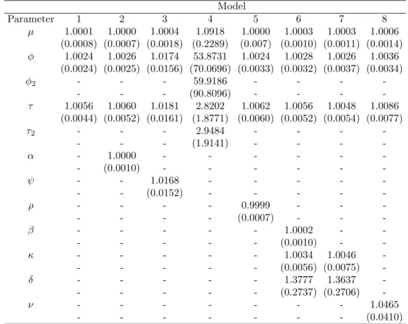
simultaneously for each simulated data set. Comparison between the two chains on the same set of data confirmed that the Markov chains are converged before the first 10,000 samples of the MCMC sampling (see Figure 4.1 for examples of the trace plots for model 6 parameters, and Table 4.1 for ˆR values). The ˆR is a relative measurement of cross-chain variances to within-chain variances, with values near 1.0 indicating good convergence (Gelman et al.,
2011). In our studies, we ran two individual Markov chains for each posterior distribution (based on a data set for a given model), and if the Markov chains do converge, the two chains for the same set of data should exhibit similar patterns after the convergence point. An ˆR value greater than 1 suggests imperfect convergence, and the bigger the ˆR value, the worse the convergence. The parameter ˆR values for the fitted models (using the simulated data) are mostly very close to one, indicating the Markov chains do converge for these models.
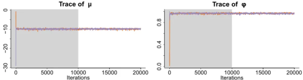
An exception, though, is the φ ( ˆR= 53.8731),τ ( ˆR = 2.8202), φ2 ( ˆR = 59.9186), and τ2 ( ˆR = 2.9484) parameters in model 4. These large values of ˆR show that the Markov chains do not converge well in this model. However, the issue is not a big concern in this particular case. In model 4, we have two independent AR(1) processes that have the same formula format. As a result, the model contains two modes. If one mode contains h(1)t , φ, τ, h(2)t , φ2, τ2 and all the other parameters, then the other mode is formed by keeping all the other parameters unchanged while exchanging the values of h(1)t ,φ, andτ altogether with h(2)t ,φ2, and τ2. Therefore, the high values of ˆR for model 4 are caused by the two chains converging to the two different modes (see Figure4.2for an example). Since the two modes are relatively far apart from each other, it is difficult for any existing sampler to explore the parameter space in this particular case. Since converging to different modes would keep the distribution of h(1)t +h(2)t unchanged, and the distribution of ˆyt only depends on the summation of h
(1) t and h(2)t , the overall model is unaffected with respect to the predictions ofyt.
The values of the fitted parameters and their standard deviations are listed in Table4.2. The results from the table show that the expected values of model parameters generally fits the profile of the data-generating parameters, which indicates a good fit.
ð ëððð ïðððð ïëððð îðððð ó í ð ó î ð ó ï ð ð Ì®¿½» ±º µ ׬»®¿¬·±²- ð ëððð ïðððð ïëððð îðððð ð òð ð òì ð òè Ì®¿½» ±º φ ׬»®¿¬·±²-ð ëððð ïðððð ïëððð îðððð ð î ì ê è Ì®¿½» ±º ׬»®¿¬·±²- ð ëððð ïðððð ïëððð îðððð ó ð òî ð òð ð òï Ì®¿½» ±º β ׬»®¿¬·±²-ð ëððð ïðððð ïëððð îðððð ð òð ð òì ð òè ï òî Ì®¿½» ±º δ ׬»®¿¬·±²- ð ëððð ïðððð ïëððð îðððð ð òð ð ð òð ì ð òð è Ì®¿½» ±ºκ
׬»®¿¬·±²-Figure 4.1: Example of trace plots of µ, φ, τ, β, δ, and κ in model 6.
The two chains in each trace plot are from two individually simulated Markov chains based on model 6 and the same set of data. The cross-chain variances is relatively small comparing to the within-chain variances after the burn-in period, indicating good convergence of the Markov chains.
0 5000 10000 15000 20000 0 .0 0 .4 0 .8 Iterations 0 5000 10000 15000 20000 0 .0 0 .4 0 .8 Iterations
trace of
2
for chain 2
trace of
2
for chain 1
trace of
for chain 1
trace of
for chain 2
Figure 4.2: Example of trace plots ofφ and φ2 in model 4 when two Markov chains converge to different modes. The φand φ2 in the trace plots are from two individually simulated Markov chains based on model 4 and the same set of data. The cross-chain variances are huge comparing to the within-chain variances due to the fact that the two chain converge to two different modes.
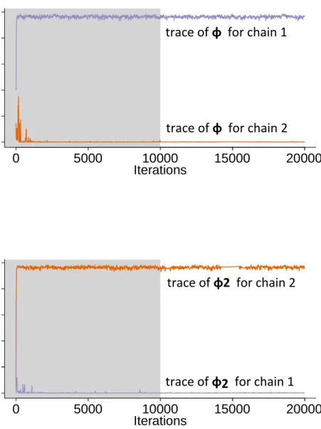
![Table 4.2: Average Parameter Estimates for Simulated Data (continued) Model Parameter Distribution 1 2 3 4 5 6 7 8 Posterior - - - - 0.0602 - - -- - - - (0.0404) - - -β Prior - - - - - 0 - -- - - - - (0.45) - -[0.1] Posterior - - - - - 0.0987 - -- - -](https://thumb-us.123doks.com/thumbv2/123dok_us/10060608.2905743/46.918.128.789.149.689/parameter-estimates-simulated-continued-parameter-distribution-posterior-posterior.webp)