Comparison of Blade Element Method and CFD Simulations of a 10 MW Wind Turbine

Comparison of Blade Element Method and CFD

Simulations of a 10 MW Wind Turbine

Galih Bangga

Institute of Aerodynamics and Gas Dynamics, University of Stuttgart, Pfaffenwaldring 21 70569 Stuttgart, Germany; [email protected], [email protected]

Academic Editor: name

Version October 12, 2018 submitted to Preprints

Abstract:The present studies deliver the computational investigations of a 10 MW turbine with a

1

diameter of 205.8 m developed within the framework of the AVATAR (Advanced Aerodynamic Tools

2

for Large Rotors) project. The simulations were carried out using two methods with different fidelity

3

levels, namely the computational fluid dynamics (CFD) and blade element and momentum (BEM)

4

approaches. For this purpose, a new BEM code namely B-GO was developed employing several

5

correction terms and three different polar and spatial interpolation options. Several flow conditions

6

were considered in the simulations, ranging from the design condition to the off-design condition

7

where massive flow separation takes place, challenging the validity of the BEM approach. An excellent

8

agreement is obtained between the BEM computations and the 3D CFD results for all blade regions,

9

even when massive flow separation occurs on the blade inboard area. The results demonstrate that

10

the selection of the polar data can influence the accuracy of the BEM results significantly, where the

11

3D polar datasets extracted from the CFD simulations are considered the best. The BEM prediction

12

depends on the interpolation order and the blade segment discretization.

13

Keywords:aerodynamics; BEM; CFD; simulation; wind turbine.

14

1. Motivation and State of the Art

15

The increased fossil fuel depletion in past decades has led to a shortage in electricity production

16

causing an increasing need in finding alternatives to fossil energy sources [1]. Wind energy has been

17

identified as one of the most promising sources for renewable energy industry [2,3]. There are two

18

main categories of wind turbines according to its rotational axis: Horizontal Axis Wind Turbines

19

(HAWTs) and Vertical Axis Wind Turbines (VAWTs). The former has been developed significantly

20

during the last decades in terms of research and commercialization.

21

Following the successful flight of Wright Brothers in 1903, researches within the aeronautical field

22

increase significantly especially in the field of propeller aerodynamics. In 1920, a German researcher

23

Betz [4] from Göttingen University developed a theory for propeller to drive the airplanes. Later, this

24

formula becomes the limit for energy extraction from the wind by simply reversing the flow of the

25

equations that is well known as the Betz limit. This implies that, even for the most ideal wind turbine,

26

the energy extracted cannot be higher than 59.3%. The performance of the turbine depends strongly

27

upon the aerodynamic design of the blades, that influences the loads acting on the rotor. It has been

28

shown from various studies that the lift driven turbine is more efficient compared to the drag driven

29

turbines [5].

30

Throughout the years, various aerodynamic modelling approaches for wind turbine simulations

31

have been developed, ranging from basic method to advanced high fidelity models. The works of Betz

32

[4] and Glauert [6] have become the founding theory for the famous blade element and momentum

33

(BEM) approach. This method, since then, has become the most widely used tool in wind turbine

34

research and industry due to its simplicity and minimal computing requirement. The method allows

35

one to perform a complete design of new blades or evaluating existing designs by utilizing the existing

36

lift and drag polar data of the airfoils constructing the blade, as described for example in [7].

37

The BEM approach models the turbine as a rotating actuator disc and the acting forces are

38

evaluated at each blade segment. There is no interaction from one to the other blade segments and the

39

method is based on the inviscid approach. As a result, the three-dimensional (3D) effects occurring

40

on the blade cannot be captured at all by the model. This is especially true near the tip and the root

41

areas. The former is caused by the flow recirculation resulting in the downwash effect and reduced

42

effective angle of attack. This effect can be modelled using a simple tip loss correction implemented in

43

the code, for example by the Prandtl tip loss correction [8], with a relatively good accuracy. On the

44

other hand, the 3D effect occurring in the root area is harder to be modelled because this involves

45

many factors including massive flow separation and three-dimensional flow behaviour. The effect is

46

widely known as rotational augmentation and has been investigated intensively since it was found by

47

Himmelskamp in 1945 [9], for example by Sörensen [10], Snel et al. [11], Du & Selig [12] and Bangga et

48

al. [1,13–16]. Under the influence of rotational augmentation, the sectional lift coefficient in the blade

49

root increases compared to the two-dimensional (2D) conditions causing the stall delay effect. The

50

centrifugal and Coriolis forces within the blade boundary layer are believed to be the main causes

51

of the phenomena for delaying the occurrence of separation. Wood [17] suggested an alternative

52

explanation that the inviscid effect is actually the main cause of the phenomenon, not the viscous effect.

53

Very recently, Bangga [13] found that both inviscid and viscous effects have their own importance for

54

the 3D rotational augmentation.

55

With the development of computing performance in the recent years, the use of the high fidelity

56

computational fluid dynamics (CFD) approach for fully resolved wind turbine rotor becomes possible.

57

This way, the three-dimensional effects occurring on the rotor blade can be physically captured. Duque

58

et al. [18] carried CFD computations of the NREL Phase VI blade using a lifting line code and a CFD

59

code that made use of overset grids and an algebraic turbulence model known as the Baldwin-Lomax

60

model, showing an improved prediction for the CFD approach compared to the lifting line model.

61

Pape and Lecanu [19] compared two turbulence models, namely the Wilcox [20] and SST models [21],

62

for wind turbine predictions. The results demonstrated that the SST model was superior compared to

63

the Wilcox model, but both were failed to accurately simulate the post-stall behaviour of the turbine

64

blade. Bangga et al. [16,22] performed CFD computations for a small MEXICO (Model Experiments

65

in Controlled Conditions) rotor [23]. They obtained a good agreement with experimental data by

66

using the Hybrid RANS/LES approach based on the SST model within the boundary layer area. They

67

observed that the 3D rotational augmentation is prominent in the root area of the rotor. It was observed

68

that the lift coefficient in the tip area reduces compared to the 2D condition due to the tip loss effect.

69

The same behaviour was also observed in [13,15]. With a sufficiently accurate CFD computation, it was

70

possible to reproduce the airfoil characteristics under rotational augmentation without using empirical

71

stall correction models.

72

One may think that there is no benefit for using the 3D polar as expensive 3D CFD computations

73

need to be done in advance. Despite that, this effort is useful when code-to-code comparison shall

74

be done in the absence of experimental data. Learning from the experience of similar comparison

75

for the AVATAR blade in [24], a significant discrepancy was obtained between different simulation

76

tools with different fidelity orders. At this point it was difficult to argue whether the differences are

77

coming from the polar data or the modelling approach. In this sense, the input polar data at least shall

78

be consistent if one intends to really assess the modelling behaviour of the method. The use of the

79

3D polar data is expected to be more beneficial for this purpose. Schneider et al. [25] documented

80

that the polar data extracted from the 3D CFD simulation of a 7.5 MW wind turbine enhanced the

81

BEM prediction significantly. A similar conclusion was obtained very recently by Guma et al. [26]

82

for a 750 kW research turbine. They observed that the origin of the polars is a crucial input that can

83

make strong difference in the results. The tangential component of the loads was proven to be harder

84

to reproduce for this case. They further indicated that the results of BEM may depend on the polar

85

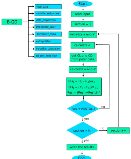
interpolation. BEM codes usually employ the linear interpolation approach, for example FAST [27]

86

and QBlade [28]. To obtain a good representation of the blade geometry and polar data, a large number

of blade elements need to be specified. This was supported by the work of Heramarwan [29] using

88

the QBlade code, especially near the tip region. Marten et al. [30] documented that the BEM results

89

linearly interpolated based on the real airfoil geometry in comparison to the direct polar data can

90

differ depending on the characteristic of the neighbouring airfoil sections. McCrink and Gregory [31]

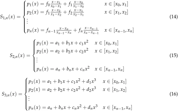
91

provided an example for the BEM calculations based on the polynomial interpolation functions in

92

MATLAB [32]. Despite that, the results were not compared to the other interpolation approaches.

93

It becomes clear that the source of the polar data and the type of interpolation used can influence

94

the blade element method predictions. Indeed these studies have been carried out long ago for wind

95

turbine applications. However, to the date there is no literature investigating the highlighted issues

96

for a very large wind turbine where the rotor diameter is greater than 200 m. The main aim of the

97

present work is to investigate the consistency of simulation tools with different fidelity levels to predict

98

the performance of a large 10 MW rotor. This becomes increasingly important as wind turbine is

99

significantly increasing in size nowadays to meet the energy demand. On the other hand, the design is

100

still based on a simple BEM model. The importance of the usage of 3D polar data and interpolation

101

order will be demonstrated in the paper. The paper is constructed as follows; the simulation approaches

102

are described in Section2, the results are discussed in Section3and all the findings are concluded in

103

Section4.

104

2. Simulation Approaches

105

2.1. Blade Element and Momentum

106

The blade element and momentum theory has its origins in momentum theory and the

107

development from this to the useful calculation tool is well explained in many texts [33–35]. The

108

general mathematical descriptions of this approach will be given in the following discussions, divided

109

into two sections. The first one is by using the momentum balance on a rotating annular stream tube

110

passing on a turbine (momentum theory). The second part is by examining the forces acting at the

111

blade elements at various sections along the blade (blade element theory). These two methods then

112

provide a series of equations that can be solved iteratively.

113

2.1.1. One dimensional momentum theory and the momentum transfer

114

The one-dimensional momentum theory that serves as a foundation for the BEM theory is

115

described in this section. This approach assumes the flow to be steady, inviscid, incompressible and

116

axisymmetric [1]. The rotor in this case can be modelled as a frictionless permeable actuator disc which

117

is assumed to impart no rotational velocity to the flow [33]. The momentum theory basically consists

118

of a control volume for conservation of mass, axial and angular momentum balances, and energy

119

conservation [36]. This surrounds the actuator disc and is bounded by a stream-tube, with two cross

120

sections far upstream and far downstream of the disc [33]. A commonly used general assumption for

121

the BEM theory is that the stream-tube is not interacting with the fluid flow outside of the evaluated

122

boundary. The modelled actuator disc extracts the energy from the stream-tube by generating an

123

axial force acting on the disc. The stream-tube enlarges downstream of the rotor plane. This causes

124

a pressure drop of the fluid flow just downstream of the disc. In the farfield region, the pressure is

125

usually assumed to reach the ambient atmospheric pressure level. In this sense, the flow velocity must

126

be smaller than the inflow speed to satisfy the Bernoulli’s equation.

127

The following equations define the energy equations upstream and downstream of the actuator

128

disc.

129

pamb+1 2ρU

2_=p

ud+1 2ρU

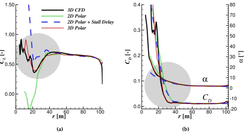
2

disc (1)

pdd+ 1 2ρU

2

disc=pamb+ 1 2ρU

2

where pamb, pud and pdd define the ambient pressure, the pressure just upstream of the disc and

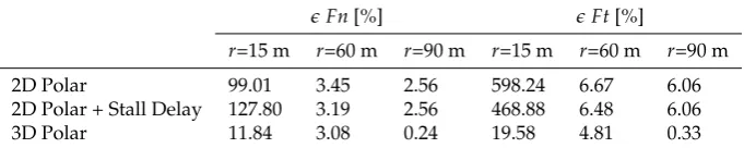
130

downstream of the disc, respectively. The velocity componentsU,UdiscandU1represent the inflow

131

velocity, the wind speed at the rotor disc and far downstream of the disc, respectively. The axial force

132

can then easily be obtained based on the pressure drop, between upstream-and-downstream-vicinity

133

of the actuator disc, derived from Equations (1) and (2) as

134

Fn= 1 2ρAdisc

U2−U₁2. (3)

Based on the momentum balance, the difference in the momentum between the upstream and

135

downstream planes of the disc must be compensated by an acting force in axial direction. In this sense,

136

the axial force can also be written in form of the flow momentum difference as

137

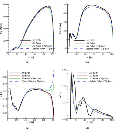
Fn =m˙ (U−U1), (4)

where the mass flow rate can be written as ˙m=ρAdiscUdisc. By comparing Equations (3) and (4), the

138

wind velocity at the actuator disc location is none other than the average velocity of the far upstream

139

and downstream the rotor plane. A new parameterais defined as the fractional reduction in flow

140

speed between the free-stream and the actuator disc.

141

a= U−Udisc

U . (5)

Then, the velocities at the rotor plane and far downstream of the disc can be redefined as a function of

142

a. The axial force in Equation (3) then can be rewritten as

143

Fn=2ρAdiscU2a(1−a). (6)

Using the axial induction factor with Equation (3), one may obtain the expression for the power

144

extraction

145

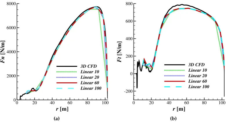
P=2ρAdiscU3a(1−a)2. (7)

According to one dimensional momentum theory, there is a pressure drop (energy lost) when the

146

wind flows through the rotor. Some of the energy loss from this axial flow is converted into rotational

147

momentum of the stream-tube, as a reaction to the rotational torque imparted to the turbine rotor thus

148

rotating annular stream tube is then introduced [1].

149

Rotating annular stream tube is shown in Figure1. Four stations are shown in the diagram, some

150

way upstream of the turbine (1), just before the blades (2), just after the blades (3) and some way

151

downstream of the blades (4). As the wind passes between stations 2 and 3, the motion of the turbine

152

causes the wind to rotate in the wake downstream of the turbine. The blade wake rotates with an

153

angular velocityωand the blades rotate with an angular velocity ofΩ. Recalling the conservation of

154

angular momentum, the torque calculation of a rotating annular element of fluid at a radiusrcan be

155

written as

156

dQ=dm˙(ωr)r=ρUdisc2πrdr(ωr)r (8) by introducing the angular (tangential) induction factorb = ω

2Ω, the elemental torque can then be

157

rewritten as

158

dQ=4b(1−a)ρUΩr2_{πrdr (9)}

2.1.2. Blade element theory

159

The blade element theory divides the rotor blade into several discrete radial elements (airfoils)

160

as described earlier in Section2.1. This theory relies on two key assumptions: (1) There are no

aerodynamic interactions between the 2D airfoil elements in different sections, and (2) the forces acting

162

on the elements are solely determined by the lift and drag characteristics of the airfoils shape and

163

relative inflow [1].

164

The definitions of the velocity vector and the lift (L) and drag (D) acting on the blade section are

165

illustrated in Figure2. The total angle between the circumferential direction to the relative inflow (V)

166

is represented by variableφ. This angle is composed by the local angle of attack (α) and the sum of the

167

pitch and twist angles (θ). The variableU_∞represents the inflow wind speed andΩis the rotational

168

speed of the turbine. Note thatU∞in Figure2is the same asUused in Section2.1.1.

169

The axial force and torque acting on the blade element can be obtained using the relations for lift

170

and drag, that are represented by the lift (CL) and drag (CD) coefficients assuming the chord length (c)

171

of the blade element is known from the geometrical model. These are formulated as following

172

dFA=N1 2ρV

2_c(C

Lcosφ+CDsinφ)dr (10)

dT =N1 2ρV

2_cr(C

Lsinφ−CDcosφ)dr. (11)

By introducing a new parameter that represents the ratio of the tangential to the inflow velocity,

173

λr = _UrΩ_∞, well known as the local speed ratio, the total flow angle can be redefined as

174

φ=tan−1

U(1−a) rΩ(1+b)

=tan−1

(1−a) λr(1+b)

. (12)

2.1.3. B-GO code description

175

A short description of the BEM code B-GO will be presented in the following section. The

176

B-GO code was written in Python language employing several commonly used packages. B-GO

177

is constructed by several subroutines that is called in the main calculations. These routines are

178

read_data, variable_assignment, data_preparation, interpolate_polar, interpolate_radial,

179

extrapolation, induction_calculation and tip_loss_correction, illustrated in Figure 3. By

180

writing each main part of the code as a subroutine, the code can be further developed in the future by

181

simply modifying only the respective functions.

182

blades

1

_{2 3}

4

Ωr(1+b)

U∞

(1-a)

V θ

ϕ

L

D ϕ

L sin ϕ - D cos ϕ

L cos

ϕ

+ D si

n

ϕ

Figure 2.Velocity vector and forces acting on the blade element.

The BEM computation is started by reading the input data. First, the axial (a) and tangential (a0)

183

induction factors are set to a small value (0.0001) to initialize the calculation. The angle of attack is

184

calculated by applying the following formula

185

α=φ−θ. (13)

CLandCDcan then be obtained from the polar data of the respective sections. Note that interpolation

186

and extrapolation of the polar data are necessary because there is a high probability that the polar data

187

does not exist for the corresponding angle of attack. The interpolation can be carried out using one

188

of the three different interpolation options that the user can choose, namely linear-, quadratic- and

189

cubic-spline interpolations. These can be expressed as:

190

S1,n(x) =

      

     

p1(x) = f0x−x1 x0−x1 +f1

x−x0

x₁−x0 x∈[x0,x1]

p2(x) = f1xx−x1−x22 +f2 x−x₁

x2−x1 x∈[x1,x2] ..

.

pn(x) = fn−1_xnx−xn₋₁−xn +fn_xnx−x−xn_n−−11 x∈[xn−1,xn]

(14)

S2,n(x) =

      

     

p1(x) =a1+b1x+c1x2 x∈[x0,x1] p2(x) =a2+b2x+c2x2 x∈[x1,x2] ..

.

pn(x) =an+bnx+cnx2 x∈[xn−1,xn]

(15)

S3,n(x) =

      

     

p1(x) =a1+b1x+c1x2+d1x3 x∈[x0,x1] p2(x) =a2+b2x+c2x2+d2x3 x∈[x1,x2] ..

.

pn(x) =an+bnx+cnx2+dnx3 x∈[xn−1,xn]

(16)

whereS1,n(x),S2,n(x)andS3,n(x)are the linear, quadratic and cubic continuous functions, respectively,

191

that interpolate the data constructed by several polynomialsp1(x),p1(x), ..,pn(x). The constants (an,

192

bn,cn,dn) shall be determined on each function for the corresponding dataset range[xn−1,xn]. Most of

193

BEM codes usually employ the linear interpolation approach. Newaanda0can be calculated using

194

a= 1

4

Cnσ

Ftipsin2φ+1

B-GO

variable_assignment read_data

data_preparation

interpolate_polar

extrapolation interpolate_radial

induction_calculation

tip_loss_correction

read input

Start

section = 1

initialize a and a'

calculate α

get CL and CD from polar data

calculate a and a'

Res1 = (ai - ai-1)/ai-1

Res2 = (a'i - a'i-1)/a'i-1

Res < RESTOL ? Res = (Res2_1+Res2₂₎0.5

section > N section++

End

no

no yes

yes

Figure 3.List of subroutines constructing the BEM code and the calculation procedure.

a0= 1

4

Ctσ

Ftipsinφcosφ−1

, (18)

where

195

Ct=CLsinφ−CDcosφ (20)

σ= cB

2πr. (21)

The Prandtl tip loss correction is given as [8]

196

Ftip= 2 π cos

−1 _e−B(R−r)

√ 1+λ2 2R

!

, (22)

whereBandRare the number of blades and the rotor radius, respectively. The obtained inductions

197

are then compared with the inductions from the previous iteration, and the residual is calculated. The

198

converge is defined when the residual is smaller than the user defined tolerance, that was set to 1 X

199

10−11for the present studies. Otherwise, 100 iterations were applied. The calculations are performed

200

for each blade section until the maximum number of blade elements ofN. The interpolation is also

201

applied to refine the evaluated segments in the radial directions, both for the polar and the blade

202

geometry, using one of the three available interpolation options as mentioned above. This allows a

203

more accurate computation to be performed.

204

In case the induction factor is higher than 0.4, the Froude momentum theory is no longer valid.

205

Spera [37] suggested a correction for the axial induction, ifa>ac, as

206

a=1+1

2K(1−2ac)− 1 2

q

(K(1−2ac) +2)2+4(Ka2c−1) (23) whereacis commonly about 0.2 andKis defined as

207

K= 4Ftipsin 2

φ

σCn . (24)

2.2. Computational Fluid Dynamics

208

The Computational Fluid Dynamics (CFD) approach is a combination of interdisciplinary fields such as physics, numerical mathematics and computer sciences to model the physical fluid flow phenomena. Turbulence is the main concern for accuracy and applicability for flow simulations using CFD. One way out of this issue is to simplify the solution variables of the Navier-Stokes equations by the Reynolds-Averaged Navier-Stokes (RANS) approach, which pose the time-averaged form of the Navier-Stokes equations. The fluid flow variables in the governing equations are subdivided into the mean and fluctuating components. For compressible flow, it is advocated to use the weighted density well known as the Favré averaging technique. This is done by utilizing the Reynolds averaging for density and pressure, yet for velocity, internal energy, enthalpy and temperature the Favré averaging procedure can be used [38–40]. The Favré averaged equation for velocity is acquired using:

˜ ui =

1 ¯ ρ T→lim∞

1 T

Z t+T

t ρuit.. (25)

equation is obtained. This mathematical expression is referred to as the Favré- and Reynolds-averaged Navier-Stokes equations [13]. In the cartesian tensor form the equations add up to

∂ρ¯ ∂t +

∂ ∂xi

(ρ¯u˜i) =0 (26)

∂

∂t(ρ¯u˜i) + ∂ ∂xj

¯ ρu˜iu˜j

= ∂p¯

∂xi

+ ∂ ∂xj

"

µ ∂u˜i ∂xj

+∂u˜j ∂xi

!#

− ∂

∂xj ˜

τ_ijRANS. (27)

The left hand side of Equation (27) accounts for the fluid momentum incorporating the variation of the mean flow with the time. This is balanced by the mean pressure gradient, viscous stresses and the apparent stress ˜τ_ijRANS, also known as the Reynolds stress (Favré-averaged) on the other side of the equation. Since the equation cannot directly be solved, the equation is remodeled to close the equation [13]. The Boussinesq hypothesis is generally taken as an approach to relate the mean velocity gradients to the Reynolds stress, for comparison see Hinze [41]. In this model the turbulent viscosity is expressed in the variableµt[13].

−τ˜_ijRANS=µt ∂u˜i

∂xj

+∂u˜j ∂xi

! −2

3

¯

pk˜+µt∂u˜k

∂xk

δij (28)

Many turbulence models are developed based on this relation through the modeling of the turbulent viscosity, commonly referred to as eddy viscosity turbulence models (EVTMs). Examples of the EVTMs are the Spalart-Allmaras (SA) model & its derivatives (1-equation),k−εmodel & the k−ωmodel & their derivatives (2-equation), and the Reynolds stress model (RSM) & its derivatives (7-equation). The shear stress transport (SST)k−ωmodel according to Menter [42] is a two-equation model family widely used in industry and research, because the model is able to deliver reasonable predictions for flows with a strong adverse pressure gradient. The model can be mathematically expressed as

∂ρk ∂t +

∂ρujk

∂xj

=P−β∗ρωk+ ∂ ∂xj

"

(µ+σ_kµt) ∂k

∂xj

#

(29)

∂ρω ∂t +

∂ρujω ∂xj

= γω νt P

−βρω2+ ∂ ∂xj

"

(µ+σωµt)

∂ω ∂xj

#

+2(1−F1)ρσω2

ω ∂k ∂xj

∂ω

∂xj. (30)

The parameters used in these equations are determined as

P=τij

ui

xj (31)

τij=µt

2Sij−

2 3ρkδij

(32)

Sij= 1 2

ui

xj

+uj xi

!

(33)

µt= ρa1k

max(a1ω,ΩF2). (34)

For the present studies, the generic 10 MW AVATAR blade [43] was chosen. The rotor is designed

209

based on the DTU 10 MW wind turbine [44] with a larger blade radius ofR= 102.9 m. The blade was

210

constructed by 6 different DU airfoils as presented in Table1. The airfoils are interpolated along the

211

blade radius, and the shapes are illustrated in Figure4. For further detail, the reader is suggested to

212

refer to [43]. The calculations were performed without tower to avoid the unsteady tower disturbance

213

effects. A Cartesian coordinate system was adopted in the present studies, where the details are

Table 1.Airfoil sections used for the AVATAR reference blade [15,43].

Airfoil Thickness [t/c] Airfoil Type

60.0% Artificial, based on thickest available DU

40.1% DU 00-W2-401

35.0% DU 00-W2-350

30.0% DU 97-W300

24.0% DU 91-W2-250 (modified fort/c=24%)

21.0% Based on DU 00-W212, added trailing edge thickness

x/c

y/

c

Figure 4.Visualization of the sectional airfoils employed in the AVATAR blade.

Figure 5.Surface mesh and detailed cross-section mesh of the blade. Variablesx,yandzrepresent local coordinate of the blade section in the rotating frame of reference.

illustrated in Figure5. In the rotating (local) coordinate system,x,yandzrepresent chordwise, normal

215

and spanwise directions of the blade which rotate together with the rotor.

216

The grid for the rotor simulations consist of several components, background (BGm), wake

217

refinement (Rm), blade (Bm) and nacelle (Nm) meshes as shown in Figure6. The blade mesh consists of

218

280x128 cells in chordwise and normal directions, respectively. The blade is discretized by 192 cells

219

along the radius with significant refinement near the root and tip areas. Figure5shows the surface

220

meshes and the sectional mesh of the blade used in the present investigations. The mesh of the blade is

221

C-H type and was constructed using the commercial grid generator Gridgen [45] with the "automesh"

Figure 6. Grid setup showing blade (purple); spinner and nacelle (red); refinement (yellow) and background grids (green). VariablesX,YandZrepresent coordinate system in the inertial frame of reference.

script developed at the institute. The 3D blade mesh was refined near the wall area satisfying the

223

non-dimensional wall distancey+ <1 to resolve the viscous sub-layer. The total resolution for the

224

complete domain reaches 39 million grid points.

225

The CFD FLOWer code [46,47] was used to numerically model the fluid flow over the rotor

226

by solving the Navier-Stokes equations on the structured meshes. A central scheme based on the

227

Jameson-Schmidt-Turkel (JST) formulation was employed for flux discretization, resulting in a second

228

order accuracy on smooth meshes. For turbulent closure, the two-equation shear stress transport (SST)

229

k−ωmodel according to Menter [42] was used. In the present analysis, fully turbulent computations

230

were carried out for the 3D rotor. The simulations were performed with the time step size of 0.037

231

s which corresponds to two degree blade revolution per physical time step. The time step can be

232

calculated as∆t[s] =∆t[°]/(Ω360°), where∆t[°]is the azimuthal time step size. Each physical time

233

step was iterated towards a pseudo steady state using 35 sub-iterations. The simulations have been

234

carried out for 11 rotor revolutions. The last one revolution was employed for the data extraction

235

purpose. The impacts of different rotor revolutions on the extracted data are shown in [13]. The basic

236

sensitivity of the CFD computations towards the blade grid and time resolutions have been presented

237

in Ref [15] and [48], respectively. For a better overview of the grid convergence studies, the results

238

of the quantified grid convergence index (GCI) according to Celik et al. [49] are presented in Table2

239

and the sectional loads are shown in Figure7. The coarse blade mesh consists of 136 cells in radial

240

direction (blade total cells number of 8.1 x 106_{), medium mesh of 192 cells (10.9 x 10}6_{) and fine mesh of}

241

272 cells (15.9 x 106). The background, wake refinement and nacelle meshes consist of 1.9 x 106, 16.34 x

242

106and 3.5 x 106cells, respectively. The grid convergence index for the fine grid is very small (less than

243

0.5%), stating that the solutions are spatially converged. It can be seen that the magnitude of power

244

and thrust for the medium and the fine grids are very close. The extrapolated relative errors are less

245

than 0.5% in both parameters, while a higher error is observed for the coarse grid due to inaccurate

246

prediction of the sectional forces in the blade inboard region. This is indicated in the sectional loads

247

predictions displayed in Figure7showing the sectional axial (Fn) and tangential force (Ft) distributions

r [m]

F

n

[

N

/m

]

0 20 40 60 80 100

0 2000 4000 6000 8000

Coarse Medium Fine

(a)

r [m]

F

t

[

N

/m

]

0 20 40 60 80 100

-200 0 200 400 600 800

Coarse Medium Fine

(b)

Figure 7.Grid density influence on the sectional loads predictions of the generic 10 MW AVATAR blade.

Table 2.Grid convergence study for the AVATAR blade using the GCI approach. Data are obtained from the URANS calculations.

Parameter Power Thrust

Value fine 9.28 x 106W 1.330 x 106N Value medium 9.26 x 106W 1.328 x 106N Value coarse 9.20 x 106W 1.326 x 106N Extrapolated rel. error

-fine 0.12% 0.27%

-medium 0.36% 0.47%

-coarse 1.02% 0.58%

Grid convercence index 0.15% 0.34%

over the radius. It can be seen clearly that the coarse grid shows a strong underestimation of the

249

sectional loads in the inboard area atr≈20 m. The main reason is that the rotational augmentation

250

effects are not well captured by the corresponding grid, that separated flow is stronger. On the other

251

hand, the medium and fine grids have similar results, indicating grid convergence. Considering the

252

accuracy and computational effort, the selection of the medium grid for CFD simulations is reasonable.

253

3. Results and Discussion

254

3.1. 3D CFD and BEM Comparison

255

This section presents the results of the comparative studies between the expensive fully resolved

256

CFD with the lower fidelity BEM computations for the AVATAR turbine. The simulations were

257

conducted at a wind speed ofU∞= 10.5 m/s, rotational speed ofn= 9.02 rpm and at zero pitch angle

258

(αp). This is the standard test case in the code-to-code comparison for the AVATAR project in [24]. To

259

avoid the necessity for 3D correction in the root area, the 3D polar data extracted from CFD simulations

260

in Ref [15] were considered in the BEM computations. The term 3D polar means that the polar data is

261

obtained directly from the 3D CFD simulations of wind turbine. In this sense, all the 3D effects are

262

already included in the polar. To demonstrate that this polar dataset is suitable for the computations,

two different polar datasets, namely the polar obtained from 2D CFD computations with and without

264

a stall delay model based on [50], are considered for comparison. The same 2D polar datasets were

265

used in [51]. The comparison is displayed in Figure8, showingFn Ftdistributions over the blade

266

radius. Note that the Prandtl tip loss correction is activated only for the 2D polar data, with and

267

without the stall delay model. It is clearly shown that the 3D CFD simulations can only be modelled

268

accurately by the use of the 3D polar dataset, especially in the root area. The pure 2D polar definitely

269

underestimates the loads in the inboard region of the blade as the 3D rotational effect is missing. The

270

use of the stall delay model improves the BEM prediction at certain regions. However, the blade

271

forces are overestimated significantly in the extreme root area forr≤20 m. A slight overestimation

272

is also observed starting forr≤40 m forFn. The quantified error of the BEM simulations relative to

273

the 3D CFD results is presented in Table3. In Figure9, the effects of the polar origin on theCL,CD

274

r [m]

F

n

[

N

/m

]

0 20 40 60 80 100

0 2000 4000 6000 8000

3D CFD 2D Polar

2D Polar + Stall Delay 3D Polar

(a)

r [m]

F

t

[

N

/m

]

0 20 40 60 80 100

-200 0 200 400 600 800

3D CFD 2D Polar

2D Polar + Stall Delay 3D Polar

(b)

Figure 8.Effects of various polar datasets on the accuracy of BEM predictions.

r [m] CL

[

-]

0 20 40 60 80 100

0.00 0.50 1.00 1.50

3D CFD 2D Polar

2D Polar + Stall Delay 3D Polar

(a)

r [m]

CD

[

-]

α

[

°]

0 20 40 60 80 100

0.0 0.1 0.2 0.3 0.4

-20 -10 0 10 20 30 40 50 60 70 80

C

D

α

(b)

andαdistributions are presented. A large discrepancy between the results is observed in the grey

275

shaded area in the root region of the blade in comparison with the 3D CFD results when the 2D polar

276

is employed. The uncorrected 2D polar underestimatesCLwhile the corrected 2D polar overestimates

277

it. It is interesting to see that an inverse behaviour is shown forα. In terms ofCD, results from the

278

2D and 2D corrected polars consistently show overpredictive values within this area. In contrast, the

279

usage of the 3D polar extracted from the 3D CFD simulations yields a consistent agreement with the

280

3D CFD data.

281

Despite the usefulness of the 3D polar, there is a limitation of its use. For example, it requires

282

the expensive 3D simulations to be carried out in advance and the tip loss effect is already present in

283

the extracted polar results. Regarding the latter, it is an advantage for BEM because this removes the

284

dependency of the calculations on the employed tip loss model, but is a side effect when a lifting line

285

approach will be used as the tip loss is calculated directly in the calculation of the induced velocity

286

itself. Therefore, a simple approach combining the 3D polar dataset with the 2D polar is suggested in

287

the present studies. The 2D polar, for example, can be applied in the region that is affected by the tip

288

loss influence. This is expected to arise starting fromr≥90 m. The evidence of this can be seen on the

289

αandCLdistributions in Figure10, indicated by the vertical lines. Figure11displays the comparison

290

of three cases; (1) 3D polar without a tip loss, (2) 3D polar with a tip loss model and (3) hybrid polar

291

with a tip loss model. It is shown that the 3D polar dataset accuracy in modelling the axial (Figure11a)

292

and tangential (Figure11b) forces near the tip area reduces as the tip loss model is activated. The use

293

of the hybrid polar is clearly able to minimize this drawback. Despite that, the hybrid polar trend is

294

clearly different than the 3D CFD results in terms of the induction distributions. Figure11cshows the

295

axial induction (a) distributions predicted using different models. It can be seen that the pure 3D and

296

Table 3.Error quantification of the sectional loads with respect to the 3D CFD data.

eFn[%] eFt[%]

r=15 m r=60 m r=90 m r=15 m r=60 m r=90 m

2D Polar 99.01 3.45 2.56 598.24 6.67 6.06

2D Polar + Stall Delay 127.80 3.19 2.56 468.88 6.48 6.06

3D Polar 11.84 3.08 0.24 19.58 4.81 0.33

r [m]

CL

[

-]

0 20 40 60 80 100

0.00 0.50 1.00 1.50 2.00 2.50 3.00

2D Polar + No Tip Loss 2D Polar + Tip Loss

(a)

r [m]

α

[

°]

0 20 40 60 80 100

-2.00 0.00 2.00 4.00 6.00 8.00 10.00 12.00 14.00 16.00

2D Polar + No Tip Loss 2D Polar + Tip Loss

(b)

r [m]

F

n

[

N

/m

]

0 20 40 60 80 100

0 2000 4000 6000 8000

3D CFD 3D Polar

3D Polar + Tip Loss Hybrid Polar + Tip Loss

(a)

r [m]

F

t

[

N

/m

]

0 20 40 60 80 100

-200 0 200 400 600 800

3D CFD 3D Polar

3D Polar + Tip Loss Hybrid Polar + Tip Loss

(b)

r [m]

a

[

-]

0 20 40 60 80 100

0.05 0.10 0.15 0.20 0.25 0.30

3D CFD 3D Polar

3D Polar + Tip Loss Hybrid Polar + Tip Loss

(c)

r [m]

a’

[

-]

0 20 40 60 80 100

0.00 0.01 0.02 0.03

3D CFD 3D Polar

3D Polar + Tip Loss Hybrid Polar + Tip Loss

(d)

Figure 11.Tip loss model influence on the 3D polar datasets.

the hybrid polar datasets predict an increasing axial induction factor near the tip when the tip loss

297

model is activated. This is caused simply by the modelling behaviour of the Prandtl tip loss factor that

298

increases the induction term in order to reduce the local effective angle of attack. A similar behaviour

299

is observed for the tangential induction (a0) distribution shown in Figure11d, but is less prominent.

300

The local drop and increase of the tangential induction in the middle and in the root area is hardly

301

captured by BEM using all polar datasets. This fluctuating behaviour is caused by the trailing vortices

302

influence within that area as demonstrated in [13,48], that surely cannot be modelled by BEM.

303

As the polar and the blade geometry has to be interpolated, the use of several interpolation

304

options in B-GO for BEM predictions is investigated. Figure12presents the influence of the linear

305

and cubic spline interpolations for polar on the BEM results. It can be seen that the effect of polar

306

interpolation is minimum if the polar data points for a blade section is sufficient. Experience has

307

shown that if the data points are limited, i.e., the polar has no enough resolution, the interpolation

308

option can determine the accuracy of the results.

The interpolation order of the blade geometry and the polar in radial direction, however, can

310

strongly influence the results as demonstrated in Figures13to16. For linear interpolation in Figure

311

13, it can be seen that the number of blade elements strongly influence the accuracy of the prediction

312

especially in the tip area of the blade. With increasing blade element number, the accuracy of the

313

computation improves. This is, however, does not hold true for the quadratic interpolation displayed

314

in Figure14. A prominent periodic change of the polar trend is shown in the middle part of the blade

315

even though though the accuracy of the results near the tip improves. Therefore, this interpolation

316

type is not recommended for further simulations. Figure15shows the effects of using the cubic

317

interpolation approach on the results. It can be seen that the accuracy improves significantly for all

318

r [m]

F

n

[

N

/m

]

0 20 40 60 80 100

0 2000 4000 6000 8000

3D CFD Linear Cubic

(a)

r [m]

F

t

[

N

/m

]

0 20 40 60 80 100

-200 0 200 400 600 800

3D CFD Linear Cubic

(b)

Figure 12.Effects of interpolation order of the polar data on the sectional force distributions along the blade radius.

r [m]

F

n

[

N

/m

]

0 20 40 60 80 100

0 2000 4000 6000 8000

3D CFD Linear 10 Linear 20 Linear 60 Linear 100

(a)

r [m]

F

t

[

N

/m

]

0 20 40 60 80 100

-200 0 200 400 600 800

3D CFD Linear 10 Linear 20 Linear 60 Linear 100

(b)

r [m]

F

n

[

N

/m

]

0 20 40 60 80 100

0 2000 4000 6000 8000

3D CFD Quadratic 10 Quadratic 20 Quadratic 60 Quadratic 100

(a)

r [m]

F

t

[

N

/m

]

0 20 40 60 80 100

-200 0 200 400 600 800

3D CFD Quadratic 10 Quadratic 20 Quadratic 60 Quadratic 100

(b)

Figure 14. Effects of blade element discretization for radial-quadratic spline interpolation on the sectional force distributions along the blade radius.

r [m]

F

n

[

N

/m

]

0 20 40 60 80 100

0 2000 4000 6000 8000

3D CFD Cubic 10 Cubic 20 Cubic 60 Cubic 100

(a)

r [m]

F

t

[

N

/m

]

0 20 40 60 80 100

-200 0 200 400 600 800

3D CFD Cubic 10 Cubic 20 Cubic 60 Cubic 100

(b)

Figure 15.Effects of blade element discretization for radial-cubic spline interpolation on the sectional force distributions along the blade radius.

blade regions by increasing the blade elements from 10 to 20. This interpolation type shows a better

319

prediction than the linear interpolation for the same amount of blade elements. This behaviour is

320

shown in Figure16where the BEM prediction using the cubic interpolation is more accurate than the

321

linear interpolation especially at the maximum axial force level in Figure16a. Therefore, the cubic

322

interpolation is suggested for further studies.

323

3.2. Simulations at Various Operating Conditions

324

In this sections, the influence of various operating conditions on the rotor performance is evaluated.

325

Figure17presents the numerical simulations of the AVATAR rotor for two different wind speeds,

r [m]

F

n

[

N

/m

]

0 20 40 60 80 100

0 2000 4000 6000 8000

3D CFD Linear 60 Cubic 60

(a)

r [m]

F

t

[

N

/m

]

0 20 40 60 80 100

-200 0 200 400 600 800

3D CFD Linear 60 Cubic 60

(b)

Figure 16.Effects of the radial interpolation order on the sectional force distributions along the blade radius.

r [m]

F

n

[

N

/m

]

0 20 40 60 80 100

0 4000 8000 12000

16000 3D CFD

BEM

20 m/s

10.5 m/s

(a)

r [m]

F

t

[

N

/m

]

0 20 40 60 80 100

0 1000 2000 3000 4000

3D CFD BEM

20 m/s

10.5 m/s

(b)

Figure 17.Sectional loads predicted by BEM and CFD for two different wind speeds. 3D polar and cubic-spline interpolation are employed.

namelyU∞= 10.5 m/s and 20 m/s. The rotational speed and pitch angle are kept constant (n= 9.02

327

rpm andαp= 0°). The higher wind speed case is characterized by massive flow separation for most of

328

the blade sections as the operating angle of attack is high, especially in the inboard area as already

329

shown in [48]. Despite that, the BEM simulations carried out in the B-GO code are able to mimic the

330

3D CFD results with an excellent agreement for the whole blade region. This indicates that the use of

331

the 3D polar data and cubic interpolation for polar and blade geometry is a suitable approach to be

332

used for wind turbine simulations at various flow situations.

333

In Figure18, the effects of tip speed ratio (λ) and pitch angle of the blade on the rotor performance

334

are evaluated. The results of the 3D CFD simulations are also presented for comparison. Three different

λ [-] CP

[

-]

4 6 8 10 12 14

0 0.1 0.2 0.3 0.4 0.5

BEM α

p = -5°

BEM α

p = 0°

BEM α

p = 5°

3D CFD α

p = 0°

(a)

λ [-] CT

[

-]

4 6 8 10 12 14

0.0 0.2 0.4 0.6 0.8 1.0 1.2

1.4 _BEM α_{p = -5°}

BEM α p = 0° BEM α

p = 5° 3D CFD α

p = 0°

(b)

Figure 18.Power and thrust coefficients at various tip speed ratios and pitch angles.

pitch angles are considered;αp= -5°, 0° and 5°. Note that positive pitch reduces the angle of attack. It

336

can be seen that the turbine power coefficientCPis about 0.2 regardless of the pitch angle value. This

337

shows that a higher pitch angle than 5° is required to control the turbine when it is operating at a wind

338

speed higher than 20 m/s, assuming the rotational speed is 9.02 rpm. With increasingλ, the power

339

coefficient value differs considerably. The smallest pitch angle generates the most mechanical power as

340

the angle of attack increases. The operating range of the turbine is also broader, from 2<λ<14, that

341

is ideal for the turbine operation. The turbine performance in terms of the power coefficient reduces

342

accordingly as the pitch angle increases to 0° and 5°. The maximum power coefficient is, however,

343

located at a similar flow situation forαp= -5° and 0° atλ≈9, while it occurs atλ ≈5.5 forαp= 5°.

344

Despite that, the increased power coefficient for the reduced pitch angle is not appearing without price.

345

The thrust coefficientCTincreases considerably for the lower pitch value than the higher one. This

346

may be dangerous for the rotor and tower structure and may reduce the lifetime of the machines.

347

4. Conclusions

348

Numerical simulations employing Blade Element and Momentum (BEM) and Computational

349

Fluid Dynamics (CFD) approaches for a large 10 MW wind turbine have been carried out. The AVATAR

350

(Advanced Aerodynamic Tools for Large Rotors) turbine with a diameter of 205.8 m developed within

351

the framework of the AVATAR project was chosen for this purpose.

352

A careful selection of the polar dataset for BEM computations is important to ensure the accuracy

353

of the results. It was shown that the 3D polar obtained from fully resolved 3D CFD simulations is the

354

most accurate dataset. The inability of the 3D polar to use the tip loss correction in BEM or ultimately

355

in the lifting line approach can be compensated by using the hybrid polar, replacing the area where

356

the tip loss appear by the 2D polar data. The accuracy of the BEM computations is also influenced

357

by the discretization of the blade segments and how they are interpolated from the existing polar

358

dataset. The studies reveal that the cubic-spline interpolation is suitable for the prediction. The linear

359

interpolation is also suitable for this purpose. However, it requires more number of blade segments to

360

achieve similar results especially in the tip area. On the other hand, the quadratic-spline interpolation

361

produces non physical oscillations of the data in the middle blade area. Thus, this is not recommended

362

to be used for later studies. Considering all the parameters above, the comparison between BEM and

363

CFD shows an excellent agreement for all blade sections even at a high wind speed case where massive

flow separation takes place in the inboard area. At last, it has been documented that the turbine

365

performance depends upon the pitch angle and tip speed ratio. The smaller pitch angle increases the

366

maximum power coefficient and rotor operating range, but the thrust force coefficient enhances as well

367

as a price. This may put more stress on the structure and can reduce the lifetime of the machine itself.

368

Funding:This research received no external funding.

369

Acknowledgments: The authors would gratefully acknowledge the follwoing institutions; the AVATAR

370

consortium for the provision of the blade geometry and the High Performance Computing Center Stuttgart

371

(HLRS) for the computational resources.

372

Conflicts of Interest:The authors declare no conflict of interest.

373

374

1. Bangga, G.; Hutomo, G.; Syawitri, T.; Kusumadewi, T.; Oktavia, W.; Sabila, A.; Setiadi, H.; Faisal, M.;

375

Hendranata, Y.; Lastomo, D.; others. Enhancing BEM simulations of a stalled wind turbine using a 3D

376

correction model. Journal of Physics: Conference Series. IOP Publishing, 2018, Vol. 974, p. 012020.

377

2. Hutomo, G.; Bangga, G.; Sasongko, H. CFD studies of the dynamic stall characteristics on a rotating airfoil.

378

Applied Mechanics and Materials2016,836, 109–114.

379

3. Bangga, G.; Lutz, T.; Dessoky, A.; Krämer, E. Unsteady Navier-Stokes studies on loads, wake, and dynamic

380

stall characteristics of a two-bladed vertical axis wind turbine. Journal of Renewable and Sustainable Energy

381

2017,9, 053303.

382

4. Betz, A. Das Maximum der theoretisch möglichen Ausnutzung des Windes durch Windmotoren.Zeitschrift

383

fur das gesamte Turbinenwesten1920,20.

384

5. Gasch, R.; Twele, J.Wind power plants: fundamentals, design, construction and operation; Springer Science &

385

Business Media, 2011.

386

6. Glauert, H.The elements of aerofoil and airscrew theory; Cambridge University Press, 1983.

387

7. Ingram, G. Wind turbine blade analysis using the blade element momentum method version 1.0.School of

388

Engineering, Durham University, UK2005.

389

8. Prandtl, L.; Betz, A. Vier Abhandlungen zur Hydrodynamik und Aerodynamik; Vol. 3, Universitätsverlag

390

Göttingen, 2010.

391

9. Himmelskamp, H.Profile investigations on a rotating airscrew; MAP, 1947.

392

10. Sørensen, J.N. Three-level, viscous-inviscid interaction technique for the prediction of separated flow past

393

rotating wing. PhD thesis, Technical University of Denmark (DTU), 1986.

394

11. Snel, H.; Houwink, R.; Bosschers, J.; Piers, W.; Van Bussel, G.; Bruining, A. Sectional prediction of 3D effects

395

for stalled flow on rotating blades and comparison with measurements. Proc. European Community Wind

396

Energy Conference, HS Stevens and Associates, LÃ1, 1993, Vol. 4.

397

12. Du, Z.; Selig, M. The effect of rotation on the boundary layer of a wind turbine blade. Renewable Energy

398

2000,20, 167–181.

399

13. Bangga, G.Three-Dimensional Flow in the Root Region of Wind Turbine Rotors; Kassel University Press GmbH,

400

2018.

401

14. Bangga, G.; Kim, Y.; Lutz, T.; Weihing, P.; Krämer, E. Investigations of the inflow turbulence effect on

402

rotational augmentation by means of CFD.Journal of Physics: Conference Series2016,753, 022026.

403

15. Bangga, G.; Lutz, T.; Jost, E.; Krämer, E. CFD studies on rotational augmentation at the inboard sections of

404

a 10 MW wind turbine rotor.Journal of Renewable and Sustainable Energy2017,9, 023304.

405

16. Bangga, G.; Lutz, T.; Krämer, E. Root flow characteristics and 3D effects of an isolated wind turbine rotor.

406

Journal of Mechanical Science and Technology2017,31, 3839–3844.

407

17. Wood, D. A three-dimensional analysis of stall-delay on a horizontal-axis wind turbine. Journal of Wind

408

Engineering and Industrial Aerodynamics1991,37, 1–14.

409

18. Duque, E.P.; Burklund, M.D.; Johnson, W. Navier-Stokes and comprehensive analysis performance

410

predictions of the NREL phase VI experiment. ASME 2003 Wind Energy Symposium. American Society of

411

Mechanical Engineers, 2003, pp. 43–61.

412

19. Pape, A.L.; Lecanu, J. 3D Navier–Stokes computations of a stall-regulated wind turbine. Wind Energy: An

413

International Journal for Progress and Applications in Wind Power Conversion Technology2004,7, 309–324.

20. Wilcox, D.C.; others. Turbulence modeling for CFD; Vol. 2, DCW industries La Canada, CA, 1998.

415

21. Menter, F.R. Two-equation eddy-viscosity turbulence models for engineering applications.AIAA journal

416

1994,32, 1598–1605.

417

22. Bangga, G.; Weihing, P.; Lutz, T.; Krämer, E. Effect of computational grid on accurate prediction of a wind

418

turbine rotor using delayed detached-eddy simulations.Journal of Mechanical Science and Technology2017,

419

31, 2359–2364.

420

23. Boorsma, K.; Schepers, J. New MEXICO experiment. Preliminary overview with initial validation Technical

421

Report ECN-E–14-048) ECN2014.

422

24. Sørensen, N.; Hansen, N.; Garcia, N.; Florentie, L.; Boorsma, K.; Gomez-Iradi, S.; Prospathopoulus, J.;

423

Barakos, G.; Wang, Y.; Jost, E.; others. AVATAR D2. 3–Power curve predictions.AVATAR project2015.

424

25. Schneider, M.S.; Nitzsche, J.; Hennings, H. Accurate load prediction by BEM with airfoil data from 3D

425

RANS simulations. Journal of Physics: Conference Series. IOP Publishing, 2016, Vol. 753, p. 082016.

426

26. Guma, G.; Bangga, G.; Jost, E.; Lutz, T.; Krämer, E. Consistent 3D CFD and BEM simulations of a research

427

turbine considering rotational augmentation. Journal of Physics: Conference Series. IOP Publishing, 2018,

428

Vol. 1037, p. 022024.

429

27. Jonkman, J.M.; Buhl Jr, M.L.; others. FAST user’s guide. National Renewable Energy Laboratory, Golden, CO,

430

Technical Report No. NREL/EL-500-382302005.

431

28. Marten, D.; Wendler, J.; Pechlivanoglou, G.; Nayeri, C.; Paschereit, C. QBLADE: an open source tool for

432

design and simulation of horizontal and vertical axis wind turbines. Int. J. Emerging Technol. Adv. Eng

433

2013,3, 264–269.

434

29. Heramarwan, H. Sensitivity of wind turbine loads to variation of aerodynamic polars predicted by BEM

435

and free vortex approaches. Bachelor’s thesis, University of Stuttgart, 2018.

436

30. Marten, D.; Pechlivanoglou, G.; Nayeri, C.; Paschereit, C. Integration of a WT Blade Design tool in

437

XFOIL/XFLR5. 10th German Wind Energy Conference (DEWEK 2010), Bremen, Germany, Nov, 2010, pp.

438

17–18.

439

31. McCrink, M.; Gregory, J.W. Blade element momentum modeling of low-Re small UAS electric propulsion

440

systems. 33rd AIAA Applied Aerodynamics Conference, 2015, p. 3296.

441

32. Li, L. MATLAB User Manual.The MathWorks, Inc., Natick, MA2001.

442

33. Masters, I.; Chapman, J.; Willis, M.; Orme, J. A robust blade element momentum theory model for tidal

443

stream turbines including tip and hub loss corrections. Journal of Marine Engineering & Technology2011,

444

10, 25–35.

445

34. Moriarty, P.J.; Hansen, A.C.AeroDyn theory manual; National Renewable Energy Laboratory Golden, CO,

446

2005.

447

35. Manwell, J.F.; McGowan, J.G.; Rogers, A.L.Wind energy explained: theory, design and application; John Wiley

448

& Sons, 2010.

449

36. Sørensen, J.N.General momentum theory for horizontal axis wind turbines; Vol. 4, Springer, 2016.

450

37. Spera, D.A. Wind turbine technology1994.

451

38. Blazek, J.Computational Fluid Dynamics - Principles and Applications; Butterworth-Heinemann, imprint of

452

Elsevier, 2015.

453

39. Jameson, A. Multigrid algorithms for compressible flow calculations. Lecture Notes in Mathematics.

454

Springer, 1986, Vol. 1228, pp. 166–201.

455

40. Favre, A. Equations des gaz turbulents compressibles, part 1 et 2. Journal de mecanique1965,4, 391.

456

41. Hinze, J. Turbulence McGraw-Hill. New York1975,218.

457

42. Menter, F.R. Two-equation eddy-viscosity turbulence models for engineering applications.AIAA journal

458

1994,32, 1598–1605.

459

43. Lekou, D.; others. Avatar deliverable d1.2 reference blade design. Technical report, ECN Wind Energy,

460

2015.

461

44. Bak, C.; Zahle, F.; Bitsche, R.; Kim, T.; Yde, A.; Henriksen, L.; Andersen, P.; Natarajan, A.; Hansen,

462

M. Design and performance of a 10 MW turbine. Technical report, Technical University of Denmark,

463

dtu-10mw-rwt.vindenergi.dtu.dk, 2013.

464

45. -. Gridgen version 15 user manual. Pointwise Inc., 2012.

465

46. Kroll, N.; Rossow, C.C.; Becker, K.; Thiele, F. The MEGAFLOW project.Aerospace Science and Technology

466

2000,4, 223–237.

47. Aumann, P.; Bartelheimer, W.; Bleecke, H.; Kuntz, M.; Lieser, J.; Monsen, E.; Eisfeld, B.; Fassbender, J.;

468

Heinrich, R.; Kroll N, Mauss M, Raddatz J, Reisch U, Roll B, Schwarz T.FLOWer installation and user manual.

469

Deutsches Zentrum fur Luft- und Raumfahrt, 2008.

470

48. Bangga, G.; Weihing, P.; Lutz, T.; Krämer, E. Hybrid RANS/LES simulations of the three-dimensional flow

471

at root region of a 10 MW wind turbine rotor. InNew Results in Numerical and Experimental Fluid Mechanics

472

XI; Springer, 2018; pp. 707–716.

473

49. Celik, I.B.; Ghia, U.; Roache, P.J.; others. Procedure for estimation and reporting of uncertainty due to

474

discretization in CFD applications.Journal of fluids Engineering2008,130.

475

50. Chaviaropoulos, P.; Hansen, M.O. Investigating three-dimensional and rotational effects on wind turbine

476

blades by means of a quasi-3D Navier-Stokes solver. Journal of Fluids Engineering2000,122, 330–336.

477

51. Bangga, G.; Guma, G.; Lutz, T.; Krämer, E. Numerical simulations of a large offshore wind turbine exposed

478

to turbulent inflow conditions. Wind Engineering2018,42, 88–96.