Page 117 www.ijiras.com | Email: [email protected]
Improving The Tracking Performance Of A Wireless Sensor
Network Using Leak Detection And Localization Technique
Onyeyilit.I.
Onohg.N.
Nwizu.U.C
Enugu State University of Science and Technology, Enugu, Nigeria
I. INTRODUCTION
In the current advent of fluid transportation (oil, water etc.) from one destination to the other, it has become a global concern (Jiagwen, Yang, and Yinfeng, 2011). Mosttimes, the carrier (pipeline) could be subjected to vandalization, rupture sabotage and corrosion. This most times result to wastage of its contents. The use of human patrol system in pipeline monitoring poses a great difficulty in detecting leakages in pipelines. This is because; the patrol team can only take observations of what is happening when they are present (Azubogu and Oguejiofor, 2013). There are many mechanisms in detecting and locating points of leak in pipeline system. Some mechanisms make use of acoustic emission which generates noises signal which can be picked up by acoustic sensors installed outside the pipeline (Wang and Hunaidi, 2004). The Oil pipeline Supervisory Control and Data Acquisition (SCADA) system for pipeline monitoring focuses on centralized data collection and control. This makes the pipeline monitoring system expensive and tedious (Azubogu and Oguejiofor 2013).
II. RELATED WORKS
LEAK POINT LOCALIZATION
Many researchers have used different techniques in locating the points of leakage in pipeline. Some combined RF signal and acoustic signal to locate a node in a WSN. Others used centralized algorithms where all computations were done by sensor nodes themselves which communicated with each other to get their position. Some algorithms rely on range measurements to estimate distance between nodes while others cannot be considered a ranged-based techniques. Many techniques are line-of-sight dependent. If there is no direct communication with the anchor nodes, its operation is limited. However, RSSI gives smaller localization error when used as a communication signal during localization. RSSI does not need extra hardware or line-of-sight to localize. A typical example is the use of RSSI in trilateration.
Abstract: Improving the tracking performance of targets in motion using low cost wireless sensor network (WSN) does not only require tracking randomly but also demands specifivity in the actual spot where there is either rupture or leak on the pipeline network. This paper proposes to develop a water pipeline test bed which can be used to experimentally simulate and detect leakages in a pipeline system in a non-invasive manner using valves and acceleration-based wireless sensor nodes. The research test bed can be used to carry out some activities which include: estimating rupture points using trilateration algorithm, measurement of network throughput, and evaluation of communication link quality, effective energy management and network security of a water pipeline network.
Page 118 www.ijiras.com | Email: [email protected]
THEORY OF TRILATERATION LOCALIZATION
ALGORITHM
To determine the actual position of the rupture in the network, trilateration localization technique is adopted in this work. Trilateration based localization algorithm is a distributed beacon-based localization algorithm; which is range-based, i.e. it uses distance estimation to compute the 2D position of the nodes in a network with the help of a communication signal from sender node to the receiving node called received signal strength indicator (RSSI). of three circles. Fig. 2.2 illustrates the computation geometry of trilateration technique.
Figure 2.2: Geometry of trilateration technique Consider the basic formular of general equation of a sphere as shown in equation (2.1)
d2 = x2 + y2 + z2
The values for x and y gives us the accurate position in two dimension for the blind node. In other to apply the above equation, the signal propagation model and power law model need to be considered. The signal propagation model shows that the received signal strength decreases with distance to the transmitter. From power law model, the mean path loss exponent is determined. Therefore, the two important values to be determined from measurement are: RSSI and path loss exponent.
III. METHODOLOGY
This paper shows an experimental performance and validation of leak detection and localization technique using wireless MEMS (Micro-Electro Mechanical System) sensor network that monitors the pipe surface acceleration in between network joints in a non-invasive manner and computes the measure of acceleration change. Six pieces of accelerometer sensor nodes were placed at uniformly spaced intervals on a water pipeline to monitor water flow. When there is leakage, there will be sudden disturbance in the water flow which induces corresponding sudden change in acceleration of the pipe vibration. This change in the pipe acceleration is measured. The location of the pipe rupture can be found in the pipe network using trilateration localization algorithm. In practice, rupture was emulated in the pipe line test bed using various valves. The emulated events include opening and closing of the water discharge valves.
EXPERIMENTAL MEASUREMENTS AND DATA
COLLECTION
The measured data at the base station during the experiment were processed in form of distribution charts and graphs subsequently analyzed.
SYSTEM IMPLEMENTATION
The designed acceleration-based sensor node was tested in the laboratory using the Shake Table method and data was recorded by the base station. The node was deployed on the developed testbed for experiments after confirming that it was working according to design specifications. The experiment was done in stages corresponding to various degrees of rupture that were emulated. Data was recorded by the Base Station when no fluid is flowing from the installed sensor nodes so as to differentiate it from when fluid is flowing in the network, and then the valves labeled V1 through V6 were adjusted
manually but sequentially to three states: closing, half-opening, and complete half-opening, Initially, all the valves were closed to allow the pressure to build up gradually, and after 240 seconds the valves were half opened sequentially and allowed to stay in that position for about 240 seconds to simulate partial rupture through V1 to V3 one after another before closing, and subsequently the valves were completely opened sequentially also for another 240 seconds to simulate full rupture through V4 to V6.
DETERMINATION OF RSSI AT VARIOUS DISTANCES
Due to the fact that the custom built sensor nodes don’t have an in-built mechanism for measuring the RSSI, calculations were made from the Friis’ equation in other to get the values of RSSI with respect to each node. Each node was assigned a different unique ID.
IV. RESULT ANALYSIS
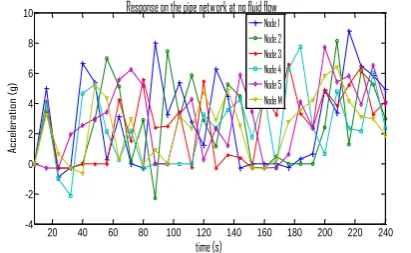
This relies on the hypothesis that rupture of considerable size in the system causes sudden expulsion of water which results in abrupt change in pipe surface vibration of the system. Also, various pipeline network conditions were examined to ascertain the magnitude of the acceleration of pipe surface at these conditions. These include: non-fluid fluid condition, fluid low condition, half-rupture and full rupture condition.
20 40 60 80 100 120 140 160 180 200 220 240
-4 -2 0 2 4 6 8 10
time (s)
Ac
ce
le
ra
tio
n
(g
)
Response on the pipe network at no fluid flow
Node 1 Node 2 Node 3 Node 4 Node 5 Node M
Page 119 www.ijiras.com | Email: [email protected] ANALYSIS OF FLUID FLOW CONDITION IN THE
PIPELINE NETWORK
Fig. 4.2 shows the plot of acceleration with time at fluid flow and valves (V1 through V6) being fully closed whereas appendix E shows the mat lab program codes. From Fig. 4.2, nodes 5 and M have the highest value of acceleration as a result of the topography of the test bed environment. These nodes were installed on pipe network which were located at sloppy terrain. This means the acceleration of the fluid flow would be high compared to that of other nodes. Node 5 has the highest acceleration (38.61g) at 170 seconds. The pipe acceleration has very high values when compared to non-flow condition in Fig. 4.1
20 40 60 80 100 120 140 160 180 200 220 240
-5 0 5 10 15 20 25 30 35 40 time (sec) Ac ce le ra ti on ( g)
Response on the Pipe Network when all Valves are Closed
Node1 Node2 Node3 Node4 Node5 NodeM
Figure 4.2: a graph of acceleration versus time at flow
FLUID FLOW IN THE PIPE NETWORK WHEN V1 WAS HALF OPENED
From Fig. 4.3, it is seen that node 1 has the highest acceleration value of 67g at exactly 90 seconds and 200 seconds. This suggests the presence of partial rupture around node 1. This relies on the hypothesis that rupture of considerable size in the system causes sudden expulsion of water, resulting in abrupt change in fluid acceleration through the pipe network. Also, the figure shows that there is a sharp change in the acceleration of the pipe surface at 98 seconds and 200 seconds when valve V1 is half opened.
20 40 60 80 100 120 140 160 180 200 220 240
-10 0 10 20 30 40 50 60 70 time (sec) A c c el er at io n ( g)
Response at Node 1 when V1 is half opened
Node1 Node2 Node3 Node4 Node5 NodeM
Figure 4.3: a graph of acceleration versus time when V1 is half opened
FLUID FLOW IN THE PIPE NETWORK WHEN V2 WAS HALF OPENED
From Fig. 4.4, it is seen that node 2 has the highest acceleration value which means there is partial rupture close to the node. There is also sharp change in the acceleration of the pipe surface at 156 seconds and 186 when V2 was half opened.
20 40 60 80 100 120 140 160 180 200 220 240
-20 0 20 40 60 80
Response at Node 2 when V2 is half opened
time (sec) A cc el era ti o n ( g) Node 1 Node 2 Node 3 Node 4 Node 5 Node M
Figure 4.4: a graph of acceleration versus time when V2 is half opened
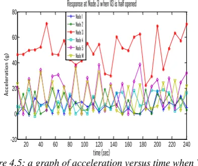
FLUID FLOW IN THE PIPE NETWORK WHEN V3 WAS HALF OPENED
From Fig. 4.5, it will be seen that node 3 has the highest acceleration values which suggest there is presence of partial rupture around the node. The Fig. 4.5 also depicts there is a sharp change in acceleration of pipe surface at 50 seconds, 78 seconds and 200 seconds.
20 40 60 80 100 120 140 160 180 200 220 240
-20 0 20 40 60 80
Response at Node 3 when V3 is half opened
time (sec) A c c e le ra ti o n ( g ) Node 1 Node 2 Node 3 Node 4 Node 5 Node M
Figure 4.5: a graph of acceleration versus time when V3 is half opened
FLUID FLOW IN THE PIPE NETWORK WHEN V4 WAS FULLY OPENED
Page 120 www.ijiras.com | Email: [email protected]
20 40 60 80 100 120 140 160 180 200 220 240
0 20 40 60 80 100 120
Response at Node 4 when V4 is fully opened
time (sec)
Ac
ce
le
ra
ti
on
(
g)
Node 1 Node 2 Node 3 Node 4 Node 5 Node M
Figure 4.6: a graph of acceleration versus time when V4 is fully opened
FLUID FLOW IN THE PIPE NETWORK WHEN V5 WAS FULLY OPENED
From Fig. 4.7, when the fluid flows through the pipeline network, and V5 is fully opened, it will be seen there is sharp change in acceleration of the fluid at exactly 104seconds, 128seconds, 155seconds 200secods with their corresponding acceleration at 139.18g, 140.34g, 141.71g, 142.75g respectively. This suggests that full rupture takes place at V5. The values of acceleration data at this node are higher than other nodes acceleration data. This is as result of the topography of the test bed environment. It shows that the node is located at sloppy terrain.
Figure 4.7: a graph of acceleration versus time when V5 is fully opened
FLUID FLOW IN THE PIPE NETWORK WHEN V6 WAS FULLY OPENED
From Fig. 4.8, when the fluid flows through the pipeline network, and V6 is fully opened, it will be seen there is sharp change in acceleration of the fluid at exactly 90seconds, 122seconds, 179seconds 200secods 210seconds and 220seconds with their corresponding acceleration at 122.36g, 139.56.g, 89.34g, 118.41g, 120.78g and 125.13 respectively. This suggests that full rupture takes place at V6. The values of acceleration data at this node are highest than other nodes acceleration data. This is as a result of the topography of the test bed environment. It shows that the node is located at sloppy terrain which validates the fact that fluid flow rate is at maximum in a sloppy terrain. The graphs show that the effect of simulated rupture in terms of acceleration depends on the distance of the rupture and the sensor locations. The closer the nodes to the point of rupture the higher the acceleration changes. The magnitude of acceleration change decreases as one moves away from the rupture point with distance. The peak values obtained are considered as the main parameter in identifying the rupture in the pipe network.
20 40 60 80 100 120 140 160 180 200 220 240
0 20 40 60 80 100 120 140
Response at Node M when V6 is fully opened
time (sec)
Ac
ce
le
ra
ti
on
(
g) Node 1
Node 2 Node 3 Node 4 Node 5 NodeM
Figure 4.8: a graph of acceleration versus time whenV6 is fully opened
ANALYSIS AND RESULT OF LOCALIZATION
ALGORITHM
From the average RSSI data collated in the table in appendix N, it will be clear that RSSI decreases with distance as a result of attenuation and other impairments. The graph of RSSI versus distance in Fig. 4.9 shows that as the RSSI decreases with distance, at a certain point, the RSSI values (-33.44 and -34.49) seem to be constant. It means that attenuation has completely set in. The mat lab code for the plotting of RSSI versus distance will appear in appendix M
25 30 35 40 45 50 55 60 65 70 75
-35 -30 -25 -20
DISTANCE (m)
R
S
S
I
(
d
B
m
)
RSSI Vs DISTANCE
Figure 4.9 Average values of RSSI versus Distance Figure 4.10 computation of path loss exponent n
Figure 4.11: Actual position of the blind node
Page 121 www.ijiras.com | Email: [email protected] Figure 4.13: Energy comparison metrics between Tilateration
GPS-based localization algorithm
Figure 4.14: Cost comparison metrics between Trilateration and GPS-based algorithm
Figure 4.15: Accuracy comparison metrics between Trilateration and GPS-based algorithm
V. CONCLUSION
From the results generated based on the experimental analysis, it is discovered that the closer the nodes to the point of rupture, the higher the acceleration change. However the magnitude of the acceleration change drastically drops based on distance from the point of rupture. Therefore location of leakage is discovered based on the sudden change in acceleration of the pipe surface vibration, thereby indicating a high value on that particular node thereby also determine the exact location based on the node involved.
Trilateration Localization Algorithm was used to discover the rupture location with the help of RSS at the receiving end. The low cost and less energy usage of the algorithm necessitated its application in leakage localization for a linear network pipeline system.
Generally, it can be deduced from the experiments and the plots that the amplitude of the acceleration depends on the level or size of the rupture and distance of rupture to the node location.
REFERENCES
[1] Ali, E., & Yuanwei, J. (2008). Monitoring of distributed pipelines systems by wireless sensor networks. Ali Eydgahi and Y IIJME International conference on information processing in sensor networks, ACM , 264-273.
[2] Azubogu, A. C., Oguejiofor, O. S., & al, e. (2013). Wireless Sensor Networks for Long distance pipeline Monitoring. World Academy of Science, Engineering and Technology , 2.
[3] Azubogu, A., & Nwalozie, G. C. (2014). Design and Implementation of pipeline monitoring system using acceleration-Based Wireless Sensor Network. International Journal of Science and Engineering , 50. [4] Ge, C., Wang, G., & Ye, H. (2008, August). Analysis of
the smallest detectable leakage flow rate of negative pressure wave-based leak detection systems for liquid pipelines. Computers And Chemical Engineering , pp. 32, 1669-1680.
[5] Isa, D., & Rajkumar, R. (2009). Pipeline defect prediction using support vector machines. Appl. Artif. Intell , 23, 758-771.
[6] Jiangwen, W., Yang, Y., & Yinfeng, W. (2011, December). School of Instrumentation science and opto-electronics engineering, Beijing University of Aeronautics and Astronautics. Retrieved March 2, 2015, from www.scirp.org/journal/articles.aspx.
[7] Jihyoung, K., Jung, S. L., Jonathan, F., Uichin, L., Luiz, V., Diego, R., et al. ( 2009). Sewersnort. Jihyoung Kim, Jung Soo LIn sixth Annual IEEE communication society conference on sensor mesh and ad hoc communications Networks (SECON) .
[8] Kamin, W., Chris, K., & David, c. (2007). A practical Evaluation of Radio Signal Strength for Ranging-based Localization. ACM international workshop on wireless sensor networks , 4.
[9] Lay-Ekuakille, A., Pariset, C., & Trotta, A. (2010). Meas. Sci. Technol . Leak detection of complex pipelines based on filter diagonalization method: Robust technique for eigenvalue assessment , 21.
[10]Lay-Ekuakille, A., Trotta, A., & Vendramin, G. (2009). FFT-Based Spectral Response for Smaller Pipeline Leak Detection. IEEE Instrumentation and
[11]Lay-Ekuakille, A., Vergallo, P., & Trotta, A. (2010). Impedance method for leak detection in zigzag pipelines. Meas. Sci. Rev , 32, 209–213.
[12]Liu, Y., Qian, Z. H., Wang, X., & Li, Y. (2010). Wireless sensor network centroid localization algorithm based on time difference of arrival. Jilin Daxue Xuebao (Gongxueban)/Journal of Jilin University (Engineering and Technology Edition) , 40, 245-249.
Page 122 www.ijiras.com | Email: [email protected] Transform . Proceedings of International Conference on
Computer, Mechatronics, Control and Electronic Engineering, Changchun, China, , 306–308.
[14]Madden, S., Nachman, L., & Stoianov, T. T. (2007). PIPENET a wireless Sensor Network for pipeline monitoring. Proceedings of the 6th international conference on information processing in sensor network, ACM , 264-273.
[15]Martins, J., & Seleghim, P. (2010). Assessment of the performance of acoustic and mass balance methods for leak detection in pipelines for transporting liquids. . ASME J. Fluids Engineering , 132.