O R I G I N A L A R T I C L E
Open Access
Spatial and temporal resolution of
geographic information: an observation-based
theory
Auriol Degbelo
1*and Werner Kuhn
2Abstract
After a review of previous work on resolution in geographic information science (GIScience), this article presents a theory of spatial and temporal resolution of sensor observations. Resolution of single observations is computed based on the characteristics of thereceptorsinvolved in the observation process, and resolution of observation collections is assessed based on the portion of the study area (or study period) that has been observed by the observations in the collection. The theory is formalized using Haskell. The concepts suggested for the description of the resolution of observation and observation collections are turned into ontology design patterns, which can be used for the annotation of current observations with their spatial and temporal resolution.
Keywords: Observation, Observation collection, Resolution, Ontology design pattern, Haskell, OWL, Spatial information theory
Introduction
Resolution is a key notion to the field of geographic infor-mation science (GIScience): it is critical in determining a data set’s fitness for a given use (see [1]), and influ-ences the patterns that can be observed during an analysis process (see [2]). In addition, as Goodchild [3] pointed out, resolution determines the volume of data which is generated and therefore the processing costs and storage volume. Finally, resolution is necessarily present in any data collection process because the world is too complex to be studied in its full detail (see for instance [1] and [4]). The literature on geographic information science and related field contains various definitions, and understand-ings of resolution. In an attempt to provide conceptual clarity, Degbelo and Kuhn [5] discussed some of these notions, and presented a framework to reconcile vari-ous connotations of the term. The framework consists ofdefinitions of resolution,proxy measures for resolution andrelated notions to resolution. Definitions of resolution refer to possible ways of defining the term; proxy mea-sures for resolution denote different meamea-sures that can be
*Correspondence:[email protected]
1Institute for Geoinformatics, University of Muenster, Muenster, Germany Full list of author information is available at the end of the article
used to characterize resolution; and related notions to res-olution denote notions closely related to resres-olution, but in fact different from it. Examples of related notions to resolution include scale, granularity and accuracy, while examples of proxy measures include the step size of a sen-sor, and the mean spacing of samples. In line with [5], resolution is defined in this article as the amount of detail (or level of detail, or degree of detail) in a representation. Resolution applies to data (i.e., representations), whereas granularity applies to conceptual models (see [4,5]). Res-olution is only one of many components of scale, with other components including extent, grain, lag, support and cartographic ratio (see [6,7]).
The transition to the digital age, and the rise of Vol-unteered Geographic Information (VGI, [8]) call for a rethinking of traditional criteria to describe the resolution of data in GIScience. The current work explores the idea of anobservation-based characterization of resolution. At least four reasons motivate this.
First, observations are key to the geo-sciences. For example, Frank [9] asserts that “all we know about the world is based on observation”. Janowicz [10] indicates that observations have been proposed as the foundation of geo-ontologies. Adams and Janowicz [11] point out that
the geosciences rely on observations, models, and simu-lations to answer complex scientific questions such as the impact of global change. Stasch et al. [12] point out that observations form the basis of empirical and physical sci-ences. The information-based ontological system outlined in [13] has, at its core, the notion of observation.
Second, observations are a central concept of the digi-tal age (which relies on information), and of VGI (where humans act as sensors to produce geographic informa-tion). Describing resolution in the era of VGI is a com-plex, underexplored, and important issue. As Goodchild [14] indicated, metrics of spatial resolution are strongly affected by the analog to digital transition. In addition (and as pointed out in [15]), mechanisms to describe the quality of human observations are needed, and are miss-ing. Describing the quality of these observations, in turn, is important to effectively assess their suitability for a given task.
Third, Frank [16] indicated that “Data quality research needs a quantitative, theory based approach. The theory must relate to the physical characteristics of the observa-tion process, where the imperfecobserva-tions in the data originate” (emphasis added). An ontology design pattern for the spa-tial data quality of observations was proposed in [17]. Yet, more specific, observation-based treatments of how spa-tial data quality components (e.g., accuracy, resolution, completeness and lineage) may be accounted for are still needed. The ultimate usefulness of an observation-based characterization of resolution is the provision of a
con-ceptual apparatus, which helps to understand semantic
differences with respect to resolution in two geographic datasets.
Fourth, a full ‘science of scale’ (as envisioned in [18]) requires progress in the understanding of resolution. As described in [18], a science of scale needs to tackle five main issues: invariants of scale, the ability to change scale, measures of the impact of scale, scale as a parameter in process models, and the implementation of multiscale approaches. Since resolution is one component of scale, measuring the impact of scale on spatial analysis requires a better understanding of resolution. Frank [19] pointed out that scale (and hence resolution) is introduced in spa-tial datasets by observation processes. Therefore, a first step towards measuring the impact of resolution of spa-tial analysis is a greater understanding ofhow resolution is introduced in observation processes. The current arti-cle attempts to provide an answer to this question, by elaborating an observation-based characterization of res-olution. The main contributions of this article are as follows:
• a brief review of previous work on resolution in GIScience;
• a formal theory of spatial and temporal resolution of observations underlying geographic information. The
theory has a dual importance: (i) at the theoretical level, it is to be taken as a small and necessary piece of the science of scale; (ii) at the practical level, the axioms of the theory (or parts of them) can be implemented, and serve the purposes of reasoning over datasets at different spatial and temporal resolution;
• a critical analysis of existing criteria for the
description of the spatial and temporal resolution of observation collections;
• ontology design patterns extending the SSN
Ontology [20]. These ontology design patterns can be used for the annotation of observations, and
observation collections of the Sensor Web with their spatial and temporal resolution.
Since GIScience has investigated resolution of
geo-graphic information for many years, Section Resolution
in GIScience: a brief review briefly reviews previous work, pointing out what is still missing. Ontology is used
as amethodto elaborate the theory, and SectionMethod
introduces the different steps followed during the devel-opment. An observation-based theory of resolution for single observations is expounded in Section Spatial and temporal resolution of a single observation, and
Section Spatial and temporal resolution of an
observa-tion collecobserva-tion discusses the resolution of observation collections. Since the spatial and temporal dimensions of geographic information are currently more understood than the thematic dimension, the theory focuses on these two as a first step (deferring a theory of observation resolution applicable to all three dimensions of geo-graphic information to future work). SectionApplications presents some examples of use of the ideas discussed.
Section Comparison with previous work discusses the
current work in relation to previous work. Section Limitations points at limitations before Section Conclusion and future workconcludes the paper.
Resolution in GIScience: a brief review
The optimum resolution: Lam and Quattrochi [24] commented on the issues of scale, resolution, and frac-tal analysis in the mapping sciences and pointed out one important research question in this context, namely‘what is the optimum resolution for a study or does an optimum really exist?’. On that subject, Marceau et al. [25] proposed and tested a method to identify the optimal resolution for a study. They concluded that (i) the concept of opti-mal spatial resolution is relevant and meaningful for the field of remote sensing, and (ii) there is a need of select-ing the appropriate resolution in any study involvselect-ing the manipulation of geographical data. Though the study was conducted in the field of remote sensing, its results are included in this literature review because they are relevant for GIScience.
Influence of resolution on other variables:Gao [26] explored the correlations between spatial resolution and root mean square error (RMSE), spatial resolution and accuracy, as well as spatial resolution and mean gradient in the context of digital elevation models (DEMs). He concluded that (i) the RMSE of a gridded DEM increases linearly with its spatial resolution from 10m to 60m, (ii) the accuracy of representing a terrain with a gridded DEM decreases as the resolution decreases from 10m to 60m, and (iii) resolution has a minimal impact on mean gradient. Deng et al. [27] used correlation and regression analysis to assess the effect of DEM resolution on cal-culated terrain attributes such as slope, plan curvature, profile curvature, north–south slope orientation, east– west slope orientation, and topographic wetness index. Their work indicated that terrain attributes respond to resolution change in different ways. Among the different terrain attributes studied, plan and profile curvatures were found to be the most sensitive attributes, and slope was the least sensitive attribute to change in resolution. The findings are valid only for landscapes found in the Santa Monica Mountains. The experiments reported in [28] revealed that there is a logarithmic relationship between DEM resolution and mean slope. Jantz and Goetz [29] examined the ability of the urban land-use-change model SLEUTH (slope, land use, exclusion, urban extent, transportation, hillshade) to capture urban growth patterns across varying spatial resolutions (i.e., cell sizes). The authors reported that, during their experiments, the amount of growth that could be produced through spontaneous growth at a resolution of 360m was more than five times the amount at a resolution of 45m. That is, the resolution of the input data impact the overall performance of an urban land-use-change model. A similar conclusion was reached by Kim [30] whose study indicated that variations in spatial and temporal resolu-tion can generate substantial differences in the outcomes of a land-use change simulation. Pontius Jr and Cheuck
[31] proposed a method which helps to examine the
sensitivity of statistical results to changes in resolution. The method was designed to facilitate multi-resolution analysis during the comparison of maps that display a shared categorical variable. Csillag et al. [32] studied the impact of spatial resolution on the classification of areas into taxonomic attributes. ‘Classification’ here means that a measurement is made at a point in space, and based on the measurement value, one would like to assign a (predefined) class to the point at which the measurement is made. Csillag et al. [32] used two examples during their study: (i) vegetation is sampled at given locations and classified according to species and/or associations; (ii) soil properties are measured at a given locations, and soil types are assigned to the locations based on the value of the measured property. They pointed out that changes in spatial resolution lead to changes in the accuracy in terms of class identification, and concluded that there may not be a single best resolution for environmental data. Finally, Lechner and Rhodes [33] recently presented a review of the effects of spatial and thematic resolution on ecologi-cal analysis. They indicated that spatial resolution affects statistical analysis outcomes such as inference about population mean, variation and statistical significance. In addition, changing spatial and thematic resolution affects the characterisation of landscapes and ecological anal-yses (e.g., measuring land cover proportions, landscape metrics and change detection). Lechner and Rhodes [33] also pointed out that spatial and thematic resolution not only have affect ecological variables, but also mutually influence one another.
Integration of resolution features and multi-resolution databases: Du et al. [34] suggested an approach to check directional consistency between rep-resentations of features at different resolutions. Examples of direction relations include east (of ), west (of ), south (of ), north (of ), southeast (of ), southwest (of ), northeast (of ), northwest (of ), and directional consistency is eval-uated by checking whether direction relations between pairs of spatial regions at different resolutions are similar. Balley et al. [35] proposed an approach to build a unified database from source databases. The source databases are databases which contain the same feature represented at different levels of spatial and thematic detail.
Formalisms for resolution: A formal framework for multi-resolution spatial data handling was suggested in
[36]. The framework has five main components: map,
thefederated multi-resolution database management sys-tem, the resolution space, the multi-resolution type and methods for aggregating resolution. Worboys [38] dealt with multi-resolution geographic spaces and proposed a formal account for multi-resolution geographic spaces using ideas related to fuzzy logic and rough set the-ory. Other formalisms for resolution, focusing on sensor observation and processes, can be found in [16] and [39] respectively. Frank [16] suggested to model (formally) the effect of resolution on the final sensor observation using a convolution with a Gaussian kernel. Weiser and Frank [39] proposed a formalism to represent multiple level of details (i.e., resolution) in discrete processes (e.g., a train ride). Finally, Bruegger [40] suggested a theory for the integration of spatial data presenting differences in spa-tial resolution and representation format (i.e., raster and vector).
Summary: In sum, there is a need of selecting the appropriate resolution in any study involving the manip-ulation of geographical data. The literature has also documented correlations between resolution and other parameters (e.g., error, accuracy, slope). This stresses the importance of choosing the appropriate resolution, and documenting the resolution at which inferences are done during an analysis. In addition, different formalisms have been suggested to model the resolution of geographic data. Yet, there is no observation-based theory of res-olution. The aim of the next section is to outline one.
The theory is proposed as an ontology, and this has
two main benefits: (i) conceptual clarification, and (ii) implementability and processability by machines (when encoded in ontology languages such as the Web Ontol-ogy Language). The latter benefit (i.e., processability by machines) is one of the advantages of the new theory over previous formalisms for resolution (and what makes the theory applicable to the Sensor Web).
Method
The steps followed in this work involve a design stage
and an implementation stage. In line with [41], the
design stage includes the identification of a motivating scenario, the identification of terms useful to describe the resolution of datasets, and the formal specification of these terms. The design stage results in a logical the-ory. The implementation stage derives a computational artifact (from the design stage), which can be used for practical tasks such as query disambiguation and query expansion. Both the motivating scenario, and terms used to describe the observation process are presented in the following subsections. The terms to describe the resolu-tion of datasets and the computaresolu-tional artifacts derived from the design stage (i.e., Ontology Design Patterns)
are introduced in Sections Spatial and temporal
reso-lution of a single observation andSpatial and temporal
resolution of an observation collection. Applications of the ontology design patterns are discussed in Section Applications. In keeping with [42], different lan-guages were used for the different phases of the
theory development. Haskell was used in the
work for the design phase (presented in Sections Spatial and temporal resolution of a single observation and Spatial and temporal resolution of an observation collection), while the Web Ontology Language was used during the implementation phase (whose results are introduced in SectionApplications). The use of different languages at different stages helps to better accommo-date the requirements of each of the phases of ontology development. As Bittner et al. [43] put it: “[o]nce one has developed a highly expressive theory, less expressive log-ics with better computational properties can be used to implement certain portions of the full theory for specific purposes”.
Motivating scenario
A collection of sensors has been deployed in a city to measure the concentration of carbon monoxide (CO) in the air. The concentration of CO is taken at different moments of the day, by different carbon monoxide ana-lyzers (COAs) placed at different locations in the city. A group of scientists is interested in analyzing the quality of the air in the city. Using the Semantic Sensor Observation Service (SemSOS), the group is able to develop an applica-tion software, which retrieves data generated by the COAs so that differences of sensors and observations regarding measurement procedures and measurement units are
har-monized. The group is now interested in extending the
semantic capabilitiesof the application so that the reso-lution of the observations is made explicit, and retrieval at different resolution, with minimal human intervention, is made possible. In particular, the group would like to know the spatial and temporal resolution of one observa-tion (Q1), and the spatial and temporal resoluobserva-tion of the observation collection produced by the COAs (Q2). Mak-ing an application software understand what ‘resolution’ of an observation (or an observation collection) means, is only possible through a formal characterization of the concept.
The scenario above presupposes the use of in-situ COAs, but remote COAs such as the MOPITT instru-ment introduced in [44] might be also used for data col-lection purposes. The theory proposed in this article takes into account both in-situ and remote sensors. For an intro-duction to SemSOS, see [45]. Q1 and Q2 are competency questions in the sense of [46].
The relevance of these analyses for the Sensor Web is at least twofold: to provide a shared conceptual basis for scientific discourse; and to provide (practical) means of representing observations generated by sensors in an information system. This section aims at selecting one of these observation ontologies as starting point for the development of the ontology of resolution. Three criteria are used to guide this choice:
• Remain neutral with respect to the distinction between field and object (C1): as mentioned in [51], the most widely accepted conceptual model for GIScience considers that geographic reality is represented either as fully definable entities (objects) or smooth, continuous spatial variation (fields). An ontology of resolution, which remains neutral to the distinction field vs object is therefore highly desirable, to ensure a wide applicability of the terms suggested in GIScience and the Sensor Web.
• Take into account humans as sensors (C2): Goodchild [8] defined Volunteered Geographic Information as the widespread engagement of private citizens in the creation of geographic information, and pointed out some valuable aspects of the information produced by volunteers: (i) the information can be timely; (ii) it is far cheaper than any alternative; and (iii) information produced by volunteers can tell about local activities in various geographic locations that go unnoticed by the world’s media. Humans acting as sensors are at the heart of VGI; the ontology of resolution should therefore be developed using a notion of sensor encompassing both instruments and humans, to be usable for both observations generated by humans and technical devices. Only ontologies capable of processing both types of observations can help to take advantage of VGI’s potential, namely, “the potential to be a significant source of geographers’ understanding of the surface of the Earth” [8]. • Take into account observation as a result and
observation as a process (C3): there has been two uses of ‘observation’ in the literature:observation as a process and observation as a result. An observation process is “an act associated with a discrete time instant or period through which a number, term or other symbol is assigned to a phenomenon” [52]. An observation result (orobservation for short) is the outcome of an observation process. The ontology of resolution should be developed in such a way that justice is done to these two senses of ‘observation’.
Table1presents the results of the application of these three criteria to the observation ontologies mentioned at the outset of this section. A detailed explanation of the results is provided in [53]. The table shows that the functional ontology of observation and measurement
Table 1Criterias C1, C2 and C3 applied to the observation ontologies
Observation ontologies C1 C2 C3
The SSN ontology of the W3C semantic sensor network incubator group [20]
Yes Yes No
The Stimulus-Sensor-Observation ontology design pattern [47]
Yes Yes No
A functional ontology of
observation and measurement [48]
Yes Yes Yes
An ontology for describing and synthesizing ecological observation data [49]
No No No
Ontological analysis of observations and measurements [50]
Yes No Yes
(or FOOM for short) is the only one which fulfills the three criteria outlined above. According to FOOM, four main entities are involved in the observation process: the particular (i.e., entity to be observed), thestimulus (i.e., detectable change in the environment), theobserver
or sensor (i.e., someone or something that provides a
symbol for a property of the particular) and the observa-tion result (i.e., a value). FOOM was formally specified using Haskell, and aligned to the foundational ontol-ogy DOLCE (Descriptive Ontolontol-ogy for Linguistic and Cognitive Engineering, see [54]). For this reason, both Haskell and DOLCE are also used while extending FOOM with concepts of spatial and temporal resolution in the next sections. Figure1illustrates the observation process. Terms useful to specify the spatial and temporal resolu-tion of sensor observaresolu-tions are highlighted in bold in the next sections.
Results
The theories of observation-based resolution are
expounded in this section. SectionSpatial and temporal resolution of a single observationdiscusses the resolution
of single observations, and Section Spatial and
temp-oral resolution of an observation collection discusses observation collections.
Spatial and temporal resolution of a single observation
The first competency question (Q1, see Section
Moti-vating scenario) is the focus of this section. As men-tioned in SectionIntroduction, resolution is a property of a representation. On that account, two terms are
introduced: spatial resolution, and temporal
Fig. 1Observation process (reprinted from [55] with permission)
approaches: a stimulus-centric approach and a property-centric approach. A stimulus-property-centric approach constrains spatial/temporal resolution using the spatial/temporal extent of the stimulus participating in the observation process. It suffers from vagueness issues regarding the determination of the spatial extent of the stimulus, and strongly depends on one’s adopted view (i.e., stimulus as process or an event) for the determination of the tempo-ral extent of the stimulus. A property-centric approach specifies resolution based on the spatial/temporal region over which the property of interest is considered homo-geneous. It avoids vagueness issues, but needs to accom-modate arbitrariness since there might be various
rea-sons for which a data provider considers the property
of interest homogeneous for his/her data collection pur-poses. To cope with both issues, our work introduces a receptor-centric approach where the spatial and tempo-ral resolution of a single sensor observation are specified based on thephysical properties of the observer. The three approaches are discussed in detail next.
The stimulus-centric approach
Stasch et al. [55] suggested to constrain the spatial and temporal resolution of an observation by the spatial and temporal extent of the stimulus. A drawback of this approach is that there is no one-way of defining the spa-tial and/or temporal extent of the stimulus involved in an observation process. For instance, in the case of a
thermometer placed in a room of area 20m2and
measur-ing the temperature, the stimulus is theheat flow of the amount of air in the room. It can be stated that the spa-tial extent of the stimulus is equal to the spaspa-tial footprint of the amount of air in the room (e.g.,20 m2), but there is no logical basis for preferring the value 20m2over smaller values of the amount of air in the room such as 15m2, 10m2 or 1m2. In fact, every size of the amount of air in the room falling within the interval ] 0, 20 ] has an equal right to be called the spatial extent of the stimulus par-ticipating in the observation process. Said another way, vagueness issues arise as to the determination of the spa-tial extent of the stimulus. As regards the temporal extent of the stimulus, its characterization is not straightforward
because, as [48] pointed out, a detectable change can be viewed as a process (periodic or continuous) or an event (intermittent). The duration of the stimulus is therefore perspective-dependent.
The property-centric approach
Frank [16] indicates that a sensor always measures over an extended area and time (called), and reports a point-observation (i.e., average value for an attribute) for this extended area and time. The extended area or time was termed thesupportof the sensor. Frank [16] ascribes sup-port to the sensor, but supsup-port has also been attributed in the literature to the observation. For instance, Atkin-son and Tate [22] define support as “[t]he size, geometry,
and orientation of the space on which the observation
is defined” (emphasis added). Modelling support as an attribute of the observation rather than of the sensor is the standpoint adopted in this work, becauseneeds not be related to the characteristics of the sensing device. As
Burrough and McDonnell ([56], page 101) pointed out,
support is the technical name used in geostatistics for the area or volume of the physical sample on which the mea-surement is made. Measuring soil pH over a physical soil
sample of 10 cm·10 cm would imply a support of 100
cm2. That is, the support is determined independently of the sensor (i.e., the instrument measuring and reporting a value for the pH of the soil at a location).
observation implies therefore a certain degree of arbitrari-ness inherent in the resolution value. The next subsection attempts to improve this situation by proposing a method to characterize the resolution of the observation based on the physical characteristics of the observer.
The receptor-centric approach
From the previous two subsections, existing criteria for observation resolution are wanting in some respects. Besides, Frank [16] pointed out in previous work that “quantitative descriptors of data quality must bejustified by the properties of the observation process” (emphasis added). That is, in the context of resolution, quantitative descriptors should be traceable to the physical proper-ties of the observation process. The introduction of a new criterion for observation resolution here aims at making progress towards fulfilling this desideratum.
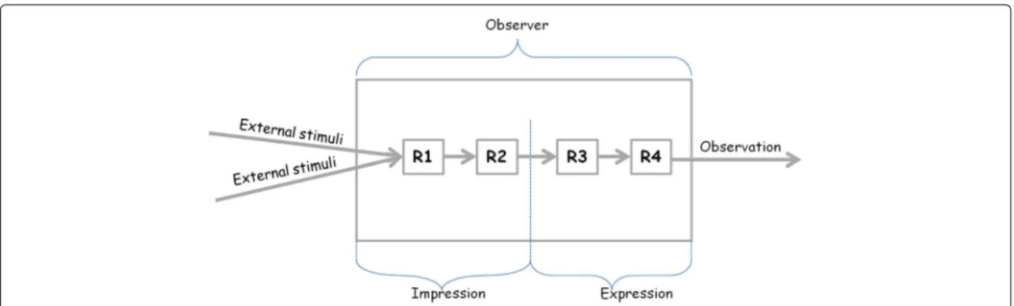
In line with [48], the observation process is concep-tualized as consisting of four steps (the first two steps are required only once, to determine the observed phe-nomenon):
Step 1: choose an observable,
Step 2: find one or more stimuli that are causally linked to the observable,
Step 3 (also called ‘impression’): detect the stimuli pro-ducing analog signals,
Step 4 (also called ‘expression’): convert the signals to observation values.
The entity which produces the analog signal upon detec-tion of the stimulus (Step 3) is called here thereceptor. Receptorsare similar to thethreshold devicesintroduced in [58], in that the production of the output (analog sig-nal) doesn’t happen immediately upon activation of the input (stimulus), but only after a short delay. However (and contrary to [59]),receptorsare not considered as the interface between the external world and the observer. In other words,receptorsdon’t need to be located at the sur-faceof the observer. It is suggested here to use the spatial region containing all the receptors stimulated during the observation process as criterion to characterize the spatial resolution of the observation. The short delay required by the receptors to produce analog signals (upon detection of the stimulus) can be used as a criterion to specify the temporal resolution of the observation.
Two new terms borrowed and adapted from neuro-science (see [60–62]) are also introduced at this point: the spatial receptive field(of the observer) and thetemporal receptive window(of the observer). Thespatial recep-tive field(SRF) is the spatial region of the observer which isstimulated during the observation process. This spatial region can be seen as two-dimensional (e.g., the palm of the hand) or three-dimensional (e.g., the whole hand) depending on the type of receptors participating in the
observation process, and hence the word ‘field’ in SRF to
reflect this fact. Thetemporal receptive window(TRW)
is the smallest interval of time required by the observer’s receptors in order to produce analog signals.
The definition of SRF above is compatible with the one ofreceptive fieldin neuroscience as a “specific region of sensory space in which an appropriate stimulus can drive an electrical response in a sensory neuron” [60]. The def-inition of TRW paraphrases and generalizes to all sensor devices the definition proposed in [61,62]. The spatial resolutionof an observation can be approximated by the spatial receptive fieldof the observer, and itstemporal resolutioncould be equated with thetemporal receptive windowof the observer participating in the observation process. There might be a chaining of different types of receptors in an observation process. In these cases, the relevant receptors for the computation of the spatial and temporal resolution are those that are stimulated by external stimuli. Figure2illustrates this point.
Examples of SRF and TRW for a single observation
With the approach introduced in Section The
receptor-centric approach, the computation of the spatial and tem-poral resolution of a single sensor observation involves three steps:
Step 1: identify the type of receptor involved in the obser-vation process;
Step 2: find the duration needed for the production of analog signal upon detection of the stimulus (rele-vant to the estimation of the TRW);
Step 3: find the size of the receptors and the number of receptors stimulated during the observation process (relevant to the estimation of the SRF).
The approach hinges on the availability of information about the receptors which participate in an observation process. This information can be found in technical docu-mentations (for sensor devices), and in research outcomes of the field of neuroscience (for human observers). The next paragraphs provide some examples of receptor, spa-tial receptive field and temporal receptive window for
human and technical observers. As said in SectionThe
Fig. 2Observer with several receptors.Note: Only receptor R1 is relevant to the estimation of the spatial and temporal resolution of the observation because it is directly stimulated by external stimuli. An example of observation process where several receptors are chained is the hearing process as described in [93]. The process can be summarized as follows:eardrums(R1) collect sound waves and vibrate; after them,hair cells(R2) convert the mechanical vibrations to electrical signals. These electrical signals are then carried to the auditory cortex, i.e., the part of the brain involved in perceiving sound. In the auditory cortex, there arespecialist neurons(R3) which specialize in different combinations of tone (e.g., some are sensitive to pure tones, such as those produced by a flute, and some to complex sounds like those made by a violin). At last, there are other neurons (R4) which can combine information from the specialist neurons to recognize a word or an instrument
the time needed for the impression operation. That is, for now, TRW is approximated using the duration of the whole observation process.
EXAMPLE 1: A Carbon Monoxide Analyzer of type
GM901 (see [63]) returns the concentration of carbon
monoxide (Observation) in a gas. The receptor of this
sensing device is themeasuring probe. Thespatial recep-tive fieldis equal to the size of the opening of the
measur-ing probe, and thetemporal receptive windowis equal
to the response time. The value of thetemporal receptive windowlies between 5 and 360 seconds. The diameter of the opening of the measuring probe varies between 300 and 500 millimeters and this suggests aspatial receptive fieldbetween 707 and 1963 square centimeters.
EXAMPLE2: A digital camera returns an image (Obser-vation), with aspatial receptive field equal to the size
of the aperture and atemporal receptive windowequal
to the shutter speed. The aperture is “the size of the adjustable opening inside the lens, which determines how much light passes through the lens to strike the image sen-sor” [64], and the shutter speed is “the amount of time the digital camera’s shutter remains open when capturing a photograph” [65]. Thereceptorof the camera is theimage sensor, but the size of the aperture determines the actual portion of the image sensor that is stimulated during the production of an image. The shutter speed determines the duration of the image sensor’s exposure to light. It is acknowledged here that resolution has been defined in the literature (for example, [66]) as a function of imag-ing aperture and the wavelength of the light. This is the optical resolution (which has sometimes also been called spatial resolution). It is inversely correlated with aperture, and measures the shortest distance between two points on
an image that can still be distinguished by the observer. However, in line with previous work [5,67], the term ‘dis-crimination’ is reserved for the shortest distance between two points on an image that can still be distinguished by the observer (the optical resolution). Approximating spatial resolution (as defined in this work, see Section Introduction) with spatial receptive field intends to inform about a different notion, and tell instead about the portion of the observer which was stimulated while producing the observation. It also reflects intuition, namely: the larger the aperture, the smaller the optical resolution (small-est details the lens can resolve), and consequently the larger the amount of spatial detail in the final image (spa-tial resolution). Further examples of receptors for tech-nical observers include thermistors (for medical digital
thermometers), bulbs (for clinical mercury
thermome-ters), telescopes (for laser altimeters), aneroid capsules (for pressure altimeters), bulbs (for psychrometers), to name a few.
EXAMPLE3: A human observer reports on a scenery at atemporal receptive windowof about 14 milliseconds (ms) using the sentence ‘there is an apple here’ (Observa-tion). The value of TRW is assigned based on the results from [68], where the authors investigated the mechanisms involved in object recognition by monkeys’ and humans’ visual systems. Keysers et al. [68] studied visual responses to very rapid image sequences composed of “color pho-tographs of faces, everyday objects familiar and unfamiliar to the subjects, and naturalistic images taken from image archives” and reported a rate of 14 ms per image for human perception and memory.
defined in [59,69] in that the observer assigns unreflec-tively on the spot a value to external stimuli. Lederman [70] indicates that, in the context of purposive exploration of the world, it typically takes 1 to 2 seconds to identify
common objects such as spoon. Therefore, thetemporal
receptive windowfor the observation ‘spoon’ in the con-text of a purposive exploration task using human hands (of blind subjects) varies between 1 and 2 seconds. The temporal receptive windowsof observations produced by human observers will depend on the observer, the type of task, and the stimulus.
EXAMPLE 5: The spatial receptive field of human observations is equal to the size of the surface stimulated during the observation process. This surface might be
cal-culated using the product N·S, where N is the number
of receptors which have participatedin the observation process, and S is the size of one receptor (if the receptors overlap, the size of the overlap should be subtracted from the product). As starting point for the computation, the
knowledge presented in Table2 can be used. Theexact
knowledge of the receptors which have participated in an observation process will become available as neuroscience evolves. For example, Krulwich [71] pointed out that it is only in 2002 that it became the new view that there is a fifth taste (umami), in addition to the four admitted during many centuries (bitter, salty, sour, sweet). This fifth taste is detected by a specific type of receptors (receptors for L-glutamate on the tongue).
Table 2Examples of receptors for a human observer
Sense Receptors, Number & Size References
Hearing eardrum(or tympanic membrane) of the ear; there is one eardrum per ear; the surface area of an eardrum is about 85 mm2
[93–95]
Sight photoreceptors of the retina; photoreceptors are about 125 million in each human eye; their diameter varies roughly between 2.5 μm and 10 μm
[93,95–97]
Smell olfactory ciliaof the olfactory neuron in the nose; there are about five million olfactory neurons in each nose, each neuron has 8-20 cilia; cilia have a length between 30 and 200 μm
[95,98,99]
Taste taste buds of the tongue; a human has between 5,000 and 10,000 taste buds; taste stimuli interact with taste buds at a small 2-10 μm region called the taste pore
[93,95,100,101]
Touch touch receptors of the skin; there are about 17,000 touch receptors in the human hand; the mean spatial receptive field of touch receptors of type FAI is about 12.6 mm2
[70,93,95]
The table illustrates that information about the type of receptors involved in an observation process, their number and their size is available from research on neuroscience and can be used to compute the spatial receptive field of the observer (and thereby estimate the spatial resolution of human observations, based on physical properties of the observers)
As this section illustrates, a receptor-centric approach to characterize the spatial and temporal resolution of a sensor observation is applicable to both in-situ (e.g., tongue) and remote (e.g., eye) sensors, and to both human and technical observers. Information given about the Carbon Monoxide Analyzer of type GM901 (tech-nical observer) was extracted from the tech(tech-nical docu-mentation of the product (see [63]). Table 2 illustrates that the (neuroscience) literature is a useful source to gather necessary information to estimate the spatial res-olution of observations produced by human observer. [68], cited previously, is an example showing that the literature on neuroscience is also a useful source to collect information for the computation of the tem-poral resolution of observations generated by human observers.
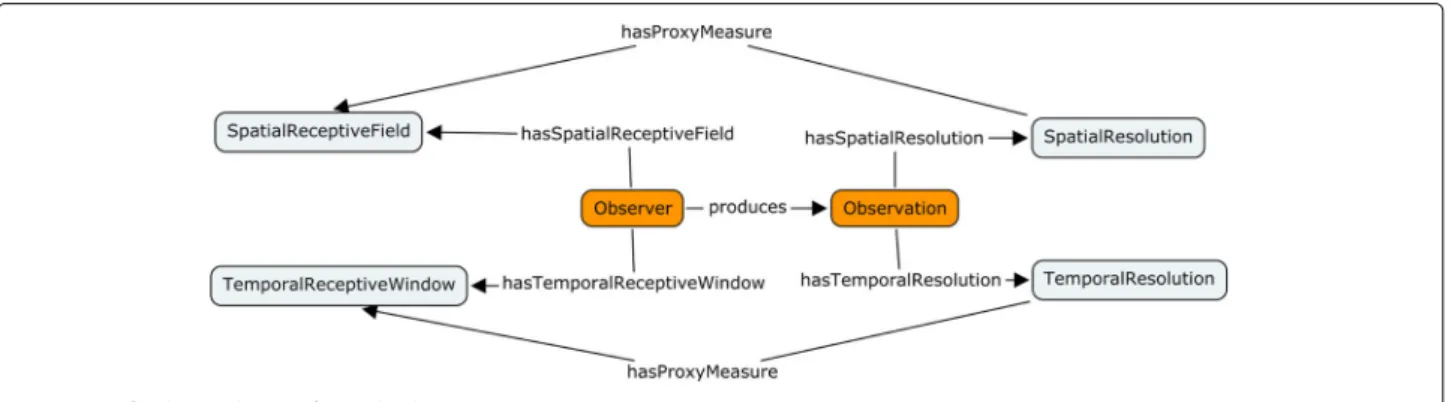
Alignment to DOLCE: resolution of an observation
‘Spatial resolution’, ‘temporal resolution’, ‘spatial receptive field’, and ‘temporal receptive window’ as characteristics of an entity (the observation or the observer) correspond
to the notion of quality in DOLCE. A quality can be
defined as “any aspect of an entity (but not a part of it), which cannot exist without that entity” [72]. Spatial receptive field and temporal receptive window inhere in the observer, and are thereforephysical qualities. Spatial receptive field and temporal receptive window are also examples ofreferential qualities, i.e., “qualities of an entity taken with reference to another entities” [73]. Both SRF
and TRW are qualities of the observer taken with
ref-erence to the stimulus. Spatial resolution and temporal resolution inhere in the observation (i.e., a social object),
and hence belong to DOLCE’s class abstract quality.
Finally, DOLCE proposes a general distinction between agentive physical objects (i.e., endurants with unity to which we ascribe intentions, beliefs and desires), and non-agentive physical objects(which are endurants which constitute these agentive physical objects). The recep-tor, being an element of the observer, is a non-agentive physical object.
Formal specification: resolution of a sensor observation The case of a carbon monoxide analyzer (COA) of type GM901 reporting a value of the concentration of
car-bon monoxide (CO) (see Example 1, SectionExamples of
Listing 1 introduces three relevant datatypes for the scenario: Magnitude (to represent the magnitude of a quality), Quale (entity evoked in a cognitive agent’s mind when observing a quality), and ObsValue (to represent observation values). For a detailed discussion of these notions, see [74].
Listing 1Definition of the datatypes Magnitude, Quale and ObsValue
−−A magnitude i n t h i s c o n t e x t i s t h e
s i z e o f a c e r t a i n r e g i o n i n a q u a l i t y s p a c e (magnitude a s Double) . T h i s i s i n
l i n e w i t h P r o b s t [ 6 1 ] who v i e w s m a g n i t u d e s a s r e g i o n s i n a c e r t a i n q u a l i t y s p a c e and c a l l s them a t o m i c q u a l i t y r e g i o n s t y p e Magnitude = Double −− magnitude a s Double
−− D e f i n i t i o n o f t h e d a t a t y p e Quale d a t a Quale = Quale Magnitude
−−An o b s e r v a t i o n v a l u e can have one o f
f o u r t y p e s : n u m e r i c a l d i s c r e t e ( r e s u l t i n g from a c o u n t i n g p r o c e s s ) ; n u m e r i c a l c o n t i n u o u s ( r e s u l t i n g from a measurement p r o c e s s − what i s measured i s t h e magnitude o f a c e r t a i n q u a l i t y ,
and measurement r e s u l t s a l w a y s come w i t h an a s s o c i a t e d measurement u n i t ) ;
c a t e g o r i c a l nominal ( c a n n o t be o r g a n i z e d
i n a l o g i c a l sequence) ; c a t e g o r i c a l o r d i n a l ( can be l o g i c a l l y o r d e r e d or
r a n k e d ) t y p e U n i t = S t r i n g −−
measurement u n i t a s S t r i n g d a t a ObsValue = Count I n t | Measure Magnitude U n i t | C a t e g o r y S t r i n g | O r d i n a l S t r i n g
The amount of air surrounding the COA is modelled as containing a certain amount (i.e., magnitude) of carbon monoxide, that is:
t y p e I d = S t r i n g −− an i d e n t i f i e r data AmountOfAir = AmountOfAir { carbonMonoxideMagnitude : :
Magnitude }
c i t y A i r = AmountOfAir
{ carbonMonoxideMagnitude = 2 . 8 }
A receptor has an id, a size, a processing time for incom-ing stimuli and a certain role. The receptor involved in the observation of the CO concentration in the city is the
measuring probe (see SectionExamples of SRF and TRW
for a single observation). It has a size and a processing time set provisionally to 1500 cm2and 60 seconds respec-tively, and the role of detecting CO molecules. The size of the receptor is set here to the size of the opening of the measuring probe (the opening of the measuring probe determines the actual portion of the measuring probe that is stimulated by external stimuli). The receptor’s role is modelled here as a description in natural language.
t y p e Area = I n t −− s p a t i a l a r e a a s I n t t y p e D u r a t i o n = I n t −− t e m p o r a l d u r a t i o n
a s I n t t y p e D e s c r i p t i o n = S t r i n g −− d e s c r i p t i o n i n n a t u r a l l a n g u a g e a s
S t r i n g
−−a r e c e p t o r can be m o d e l l e d a s h a v i n g
an id, a s i z e , a p r o c e s s i n g t i m e f o r incoming s t i m u l i , and a c e r t a i n r o l e
d a t a R e c e p t o r = R e c e p t o r { r e c e p t o r I d : : Id , r e c e p t o r S i z e : : Area , p r o c e s s i n g T i m e
: : D u r a t i o n , r o l e : : D e s c r i p t i o n } m e a s u r i n g P r o b e = R e c e p t o r { r e c e p t o r I d =
‘ ‘ re1 ’ ’ , r e c e p t o r S i z e = 1 5 0 0 , p r o c e s s i n g T i m e = 6 0 , r o l e = ‘ ‘ d e t e c t i o n o f CO m o l e c u l e s ’ ’ }
An observer has an id and a number of receptors of a certain type. It carries a quale and an observation value. The measurement unit used below for observation values is “ppm” standing for parts per million. For simplicity, it is assumed here that all receptors (with a similar function) have the same size, and there is no malfunction during the observation process (i.e., either all the receptors detecting the stimulus are stimulated or none of them). The assump-tion that all receptors have the same size is in line with Quine [59] who states: “The subject’s sensory receptors are fixed in position, limited in number, and substantially alike”. A COA has one measuring probe.
d a t a O b s e r v e r = O b s e r v e r { o b s e r v e r I d : : Id , r e c e p t o r : : R e c e p t o r ,
numberOfReceptors : : I n t, q u a l e : : Quale , o b s e r v a t i o n V a l u e : : ObsValue } c o A n a l y z e r = O b s e r v e r { o b s e r v e r I d =
‘ ‘ ob1 ’ ’ , r e c e p t o r = m e a s u r i n g P r o b e , numberOfReceptors = 1 , q u a l e = Quale 0 . 0 , o b s e r v a t i o n V a l u e =
Measure 0 . 0 ‘ ‘ ppm ’ ’ }
Listing2presents the alignment of the terms ‘observer’ and ‘receptor’ to DOLCE.
Listing 2Alignment of observer and receptor to DOLCE
c l a s s PHYSICAL_ENDURANTS p h y s i c a l E n d u r a n t c l a s s
PHYSICAL_ENDURANTS p h y s i c a l O b j e c t =>
PHYSICAL_OBJECTS p h y s i c a l O b j e c t c l a s s
PHYSICAL_OBJECTS a g e n t =>
AGENTIVE_OBJECTS a g e n t −− a g e n t i v e
p h y s i c a l o b j e c t s c l a s s PHYSICAL_OBJECTS nonAgent => NON_AGENTIVE_OBJECTS nonAgent −− non−a g e n t i v e p h y s i c a l
o b j e c t s
−− Q u a l i t i e s have h o s t s i n which t h e y
i n h e r e c l a s s QUALITIES q u a l i t y e n t i t y
where
h o s t : : q u a l i t y e n t i t y −> e n t i t y
−−an o b s e r v e r i s an a g e n t i v e
p h y s i c a l o b j e c t i n s t a n c e
PHYSICAL_ENDURANTS O b s e r v e r i n s t a n c e
PHYSICAL_OBJECTS O b s e r v e r i n s t a n c e
AGENTIVE_OBJECTS O b s e r v e r
−−a r e c e p t o r i s a non−a g e n t i v e p h y s i c a l
o b j e c t i n s t a n c e PHYSICAL_ENDURANTS R e c e p t o r i n s t a n c e PHYSICAL_OBJECTS R e c e p t o r i n s t a n c e NON_AGENTIVE_OBJECTS
R e c e p t o r
and this leads to a spatial and temporal resolution for the quale. The spatial resolution of the quale is modelled in the current work as being equal to the spatial receptive field of the observer involved in the perception operation. The temporal resolution of the quale is equal to the tem-poral receptive window of the observer which participated in the perception of the observed quality. The function magnitudeToQuale establishes a mapping from a certain magnitude to the corresponding quale, and more details about it are provided below.
−− d e f i n i t i o n o f t h e q u a l i t y c a r b o n
monoxide d a t a PHYSICAL_ENDURANTS p h y s i c a l E n d u r a n t => CarbonMonoxide p h y s i c a l E n d u r a n t = CarbonMonoxide p h y s i c a l E n d u r a n t i n s t a n c e QUALITIES CarbonMonoxide AmountOfAir where
−− t h e h o s t o f t h e c a r b o n monoxide
q u a l i t y i s t h e amount o f a i r
h o s t ( CarbonMonoxide amountOfAir ) = amountOfAir
−− S t i m u l u s a s a p r o c e s s which i n v o l v e s
a q u a l i t y and an a g e n t c l a s s ( QUALITIES q u a l i t y e n t i t y , AGENTIVE_OBJECTS a g e n t ) => STIMULI q u a l i t y e n t i t y a g e n t
where
−− p e r c e p t i o n a s a b e h a v i o u r , t h a t t a k e s
a s i n p u t a s t i m u l u s , and r e t u r n s a s o u t p u t a q u a l e t h a t i s c a r r i e d by an a g e n t
p e r c e i v e : : q u a l i t y e n t i t y −> a g e n t −> a g e n t
i n s t a n c e STIMULI CarbonMonoxide AmountOfAir O b s e r v e r where
p e r c e i v e ( CarbonMonoxide amountOfAir ) o b s e r v e r = o b s e r v e r { q u a l e =
magnitudeToQuale ( carbonMonoxideMagnitude amountOfAir ) }
Based on the quale, the observer produces an obser-vation value. The function qualeToMeasure introduced below establishes a mapping between a quale and an observation value (resulting from a measurement process).
−− O b s e r v a t i o n a s a p r o c e s s which
i n v o l v e s a q u a l i t y and an a g e n t
c l a s s STIMULI q u a l i t y e n t i t y a g e n t =>
OBSERVATIONS q u a l i t y e n t i t y a g e n t where
o b s e r v e : : q u a l i t y e n t i t y
−> a g e n t −> a g e n t
i n s t a n c e OBSERVATIONS CarbonMonoxide AmountOfAir O b s e r v e r where
o b s e r v e ( CarbonMonoxide amountOfAir ) o b s e r v e r = o b s e r v e r { q u a l e = q u a l e
( p e r c e i v e ( CarbonMonoxide amountOfAir ) o b s e r v e r ) ,
o b s e r v a t i o n V a l u e = qualeToMeasure ( q u a l e ( p e r c e i v e ( CarbonMonoxide
amountOfAir ) o b s e r v e r ) ) }
The spatial resolution and the temporal resolution of the observation value are now equated with the spatial reso-lution and temporal resoreso-lution of the quale respectively1.
−− t h e s p e c i f i c a t i o n o f t h e r e s o l u t i o n o f an o b s e r v a t i o n n e c e s s i t a t e s
t h e o c c u r r e n c e o f t h e o b s e r v a t i o n
c l a s s OBSERVATIONS q u a l i t y e n t i t y a g e n t
=> OBSERVATION_RESOLUTIONS q u a l i t y e n t i t y a g e n t where
−− s p a t i a l r e s o l u t i o n o f an o b s e r v a t i o n
v a l u e ( w i t h r e f e r e n c e t o a
c e r t a i n q u a l i t y ) i s an a r e a . The o b s e r v a t i o n v a l u e i s c a r r i e d by
t h e a g e n t
s p a t i a l R e s o l u t i o n O b s e r v a t i o n : : q u a l i t y e n t i t y −> a g e n t −> Area
−− t e m p o r a l r e s o l u t i o n o f an o b s e r v a t i o n
v a l u e ( w i t h r e f e r e n c e t o a
c e r t a i n q u a l i t y ) i s a d u r a t i o n . The o b s e r v a t i o n v a l u e i s c a r r i e d
by t h e a g e n t
t e m p o r a l R e s o l u t i o n O b s e r v a t i o n : : q u a l i t y e n t i t y −> a g e n t −>
D u r a t i o n
i n s t a n c e OBSERVATION_RESOLUTIONS CarbonMonoxide AmountOfAir O b s e r v e r
where
−− s p a t i a l r e s o l u t i o n o f an o b s e r v a t i o n
i s e q u a l t o t h e s p a t i a l
r e c e p t i v e f i e l d o f t h e o b s e r v e r s p a t i a l R e s o l u t i o n O b s e r v a t i o n
( CarbonMonoxide amountOfAir ) o b s e r v e r = s p a t i a l R e c e p t i v e F i e l d ( p e r c e i v e ( CarbonMonoxide amountOfAir )
o b s e r v e r )
−− t e m p o r a l r e s o l u t i o n o f an o b s e r v a t i o n
i s e q u a l t o t h e t e m p o r a l
r e c e p t i v e window o f t h e o b s e r v e r t e m p o r a l R e s o l u t i o n O b s e r v a t i o n
( CarbonMonoxide amountOfAir ) o b s e r v e r = t e m p o r a l R e c e p t i v e W i n d o w ( p e r c e i v e ( CarbonMonoxide amountOfAir )
o b s e r v e r )
Spatial receptive field is now specified as the size of the spatial region containing all receptors stimulated during the observation process. Temporal receptive window is the processing time of the receptors stimulated during the observation process.
s p a t i a l R e c e p t i v e F i e l d : : O b s e r v e r
−> Area
s p a t i a l R e c e p t i v e F i e l d o b s e r v e r = numberOfReceptors o b s e r v e r ∗
r e c e p t o r S i z e ( r e c e p t o r o b s e r v e r )
t e m p o r a l R e c e p t i v e W i n d o w : : O b s e r v e r
−> D u r a t i o n
t e m p o r a l R e c e p t i v e W i n d o w o b s e r v e r = p r o c e s s i n g T i m e ( r e c e p t o r o b s e r v e r )
qualeToMeasure is a monotonic function. In the context of the current scenario, these two functions will be given a simple definition, assuming an approximation factor of the magnitude amounting to 0.9 during the mapping magnitudeToQuale, and another approximation factor of 0.9 during the mapping qualeToMeasure.
a F a c t o r = 0 . 9 : : Double
−− t h e a p p r o x i m a t i o n f a c t o r i s
i n t r o d u c e d t o r e f l e c t t h e f a c t t h a t q u a l i a a p p r o x i m a t e a b s o l u t e m a g n i t u d e s
magnitudeToQuale : : Magnitude −> Quale magnitudeToQuale magnitude = Quale (magnitude ∗ a F a c t o r )
−− t h e u n i t a s s o c i a t e d w i t h o b s e r v a t i o n
v a l u e s i n t h i s example i s ‘ ‘ ppm ’ ’ .
−− t h e r e i s a f u r t h e r a p p r o x i m a t i o n o f
t h e magnitude d u r i n g t h e e x p r e s s i o n p r o c e s s
qualeToMeasure : : Quale −> ObsValue qualeToMeasure ( Quale magnitude) = Measure (magnitude ∗ a F a c t o r ) ‘ ‘ ppm ’ ’
The Haskell specification presented above is available athttps://doi.org/10.5281/zenodo.1293285. As argued in
Winter and Nittel [75], a running Haskell
specifica-tion guarantees theconsistency(i.e., internal consistency between the concepts in the specification), correctness (i.e., the developer has said what he intended to say),
and completeness (i.e., appropriate coverage of
ques-tions within a domain) of the specification. The theory expounded above is thus consistent, correct, and complete with respect to the question Q1 (how to specify the res-olution of an observation using the characteristics of the observed entity, the stimulus, and the sensor?). All con-cepts suggested to model the resolution of single observa-tions have also been implemented as an ontology design pattern (ODP) in the Web Ontology Language (OWL).
The ODP is an extension to the SSN Ontology [20] and
offers concepts needed to annotate single observations with their resolution. The ODP for the resolution of single observations is shown in Fig.3, and can be downloaded at: https://doi.org/10.5281/zenodo.1293285.
Spatial and temporal resolution of an observation collection
The second competency question (Q2, see Section Motivating scenario) is put under scrutiny in this section. ‘Spatial resolution’ and ‘temporal resolution’ denote the amount of spatial detail in the observation collection, and the amount of temporal detail in the observation collec-tion respectively. An observacollec-tion colleccollec-tion is a colleccollec-tion of single observations (or ‘observations’ for short). Wood and Galton [76] presented a review of existing ontologies (including DOLCE and the Basic Formal Ontology) for the representation of collectives (‘collective’ from [76] is equivalent to ‘collection’ in this article), and proposed a taxonomy allowing the classification of around 1800 dis-tinct types of collectives. Adapting their reflections to the specific case of collections of observations leads to the following statements:
• An observation collection is aconcrete particular, not a type, nor an abstract entity;
• An observation collection is acontinuant, that is, it is to be thought of as enduring over a period of time, existing as a whole at each moment during that period, and possibly undergoing various types of change over that period;
• An observation collection has multiple observations (and only observations) asmembers. In line with [77], themember-collection relationship is a more specific kind ofpart-of relation. Winston et al. [77] also point out that membership in a collection is determined based on one of two factors: spatial proximity or social connection. As regards observation collections, membership in an observation collection is
determined based onsocial connection (not spatial proximity).
In addition, the current work adopts the standpoint that an entity iseithera single observationoran observation collection. It cannot be both. Put differently, an obser-vation collection has n members, where n is a natural
number greater than one. An observation collection with only one observation is a single observation. In that sense, one remote sensing image is not an observation collec-tion, but two consecutive pictures of an area (are already enough to) form an observation collection.
Observation collections and observations are social objects in the sense of the DOLCE Ultra Light (DUL) upper ontology2. There is however one important differ-ence between the two which relates to their process of generation: an observation is generated by observing the physical reality3; an observation collection is produced by gathering other social objects (i.e., observations). In terms of DUL, an observation collection can be viewed as a DUL:Configuration (‘A collection whose members are organized according to a certain schema that can be represented by a Description’) while an observation may be regarded as a DUL:Situation (‘A relational context created by an observer on the basis of a Description’).
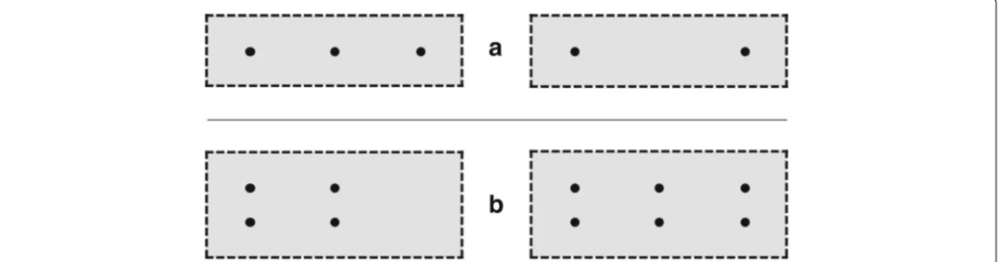
Figure4shows four examples of observation collections. Two criteria suggested in previous work - spacing and cov-erage - can be used to characterize the spatial resolution of the observation collections. These two criteria are criti-cally discussed in the next two paragraphs. The arguments brought forward for the spatial resolution hold,mutatis mutandis, for the temporal resolution of the observation collections.
Spacing: Goodchild and Proctor [1] mentioned the spacing of the points (i.e., observations) as a criterion to characterize the spatial resolution of observation col-lections. The estimation of spacing necessitates some information about the spatial location of each observa-tion. Spacing can be calculated in (at least) four ways:
the maximum spacing, the minimum spacing, the total
spacing and the mean spacing. All four have some
dis-advantages. For example, themaximum spacing and the
minimum spacingsay nothing about how the observation
collection is spatially detailed. They rather tell that, within the current observation collection, the closest locations are within a distance equal to theminimum spacing, the
farthest within a distance equal to themaximum
spac-ing. Regarding thetotal spacing, one disadvantage is the need to specify a spatial ordering for the observation col-lection. As discussed in [53], this choice might involve some arbitrariness. The ultimate implication of the use of total spacing as criterion, is that a decision-maker will be provided with different values of spatial resolution for an observation collection, with no means to decide which one to choose for his or her purpose. In addition,
there are cases such as the one from Fig. 4awhere the
total spacing fails to capture the fact that two observation collections have different amounts of spatial detail. It is indeed arguable that (under the assumption that the size of the points is negligible) the two observation collections from Fig.4ahave the same spacingS. The use of themean spacinghas the advantage that it is no longer necessary to define what observation is the first, and what is the next. However, a serious drawback of this criterion is that, when applied to the observation collections from Fig.4b, it gives the same value. In other words, this criterion fails to cap-ture the fact, as far as Fig.4bis concerned, the observation collection further right is spatially more detailed than the observation collection further left.
Coverage: coverage, proposed in [78], is another crite-rion that can be used to characterize the spatial resolution of observation collections. The value C of this criterion for the observation collections presented in Fig.4is:
C= N·A
E
where N is the number of observations, A is the area covered by each observation, and E is the extent of the study area. This criterion will yield different values for
the spatial resolutions of the observation collections from Fig. 4a-b, capturing the fact that these observation col-lections have different amounts of spatial detail. There is also no need to face the arbitrariness which comes with the specification of a spatial ordering for an observation collection, and C gives an immediate impression of the portion of the study area which has been observed. A drawback of this criterion is that it leads to a dimen-sionless value, and this fails to account for the intuition (reflected in expressions such as ‘10 meters resolution’, ‘20 meters resolution’, and so on) that resolution is a property to which humans associate a dimension of length.
From the previous paragraphs, spacing and coverage as criteria to characterize the spatial/temporal resolution of observation collections are wanting in some respects. As a general requirement for the Sensor Web and GIScience, proxy measures for the spatial/temporal resolution of observation collections should: (i) avoid the arbitrari-ness ensuant on the necessity to define a spatial ordering for the observation collection; (ii) have the dimension of length/time4.; and (iii) mirror the fact that a perfect sampling strategy covers the whole study area/period. This motivates the introduction of the following two terms for the description of the resolution of observation
collections: observed study area and observed study
period. The observed study area is the portion of the
study area that has been observed. Theobserved study
period is the portion of the study period that has been observed. The study area is the spatial extent of the anal-ysis and the study period is the temporal extent of the analysis.
Observed study area and observed study period
Theobserved study areaof an observation collection can be obtained by summing up theobserved areas of each of the observations of the collection. Theobserved areaof anobservationis the spatial region of the phenomenon of interest that has been observed. LetRSumbe defined after [79] as the sum of two spatial regions.RSumis similar to the operatorunionused in set theory in that theRSumof two regions A and B is a region C such that all the elements belonging to C either belong to A, or B or both A and B. TheRSumof two regions is itself a region (see [79] for the formalization). The following equation holds:
ObservedStudyArea=RSumni=1[ai]
whereai denotes the observed area of each observation,
and n is the number of observations in the observation collection.
Likewise, theobserved study periodof an observation
collection can be obtained by summing up theobserved
periods of each of the observations in the observation col-lection. Theobserved periodof asingle observationis the
temporal region of the phenomenon of interest that has been observed.
ObservedStudyPeriod=RSumni=1[wi]
wherewidesignates the observed period of each
tion, and n is the number of observations in the observa-tion collecobserva-tion.
Modelling the resolution of an observation collection The spatial resolution and temporal resolution of the observation collection (Q2) can be equated with the observed study area, and the observed study period respectively. The observed study area provides the decision-maker with a value which reflects how much of the study area has effectively been observed (or sam-pled). Its value is independent of the ordering of the observations, and also independent of the type of sam-pling strategy (i.e., regular vs irregular). The observed areas of the individual observations in the collection need not be alike (some might be greater or smaller than oth-ers). Theobserved study areahas a dimension of length squared, but a linear measure can be obtained by tak-ing the square root. For a given study area, the equation ObservedStudyArea= RSumni=1[ai] will approximate the
study area if n tends to infinity (and under the sufficient condition that theaiare disjoint).
The observed study area and the observed study period are more suitable than spacing and coverage to characterize the spatial and temporal resolution of observation collections. The fulfill the three require-ments for proxy measures for resolution listed above, thereby addressing shortcomings of criteria suggested in previous work. In addition, decision-makers are free to compute the proportion of the study area/study period that has effectively been observed through the ratios
ObservedStudyArea StudyArea or
ObservedStudyPeriod StudyPeriod .
If the observed area is defined as spatial reference field, and the observed period as temporal receptive
win-dow, a computation of theobserved study areaand the
and temporal supports may be used as criteria to charac-terize the observed area and observed period and
com-pute theobserved study areaandobserved study period
(one should be aware of supports’ drawbacks discussed in SectionThe property-centric approachthough).
A minor drawback of these two criteria is that their full significance is only unfolded when the extent of the whole study area/period is known. For example, stating that the observed study periodof an observation collection isone hoursays nothing about the actual quality of the obser-vation collection, unless the whole temporal extent under consideration (e.g., one day or one month) is also made explicit. The extent of the study area/period will also be required for a meaningful comparison of two observa-tion collecobserva-tions with respect to their spatial and temporal resolution. Even so, this drawback is not intrinsic to the criteria suggested. It is rather a consequence from the gen-eral fact that values need some context if their significance is to be assessed. Another minor drawback of these two criteria is that they arenew, and thus yet to be adopted by the practice of metadata documentation. However, the lack of criteria in the literature which fulfill the three characteristics mentioned in SectionSpatial and temporal resolution of an observation collectionsuggests that the Sensor Web and GIScience should come up with new cri-teria to describe the resolution of observations collections (rather than conforming to existing ones).
Alignment to DOLCE: resolution of an observation collection In line with [80], an ‘observation collection’ is viewed as a social object. A social object is an object that exists only within a process of social communication, in which at least one PhysicalObject participates. ‘Spatial resolution’, ‘temporal resolution’, ‘observed study area’, ‘observed study period’, ‘observed area’ and ‘observed period’ are all qual-ities that inhere in a social object, and thereforeabstract
qualities. Figure 5 shows the ODP for the resolution
of observation collections which summarizes all terms
introduced in this section. The ODP can be downloaded athttps://doi.org/10.5281/zenodo.1293285.
Applications
This section presents the practical usefulness of some of the ideas presented in this work. As discussed in [41], practical usefulness is an evaluation criterion of the implementation stage of ontology development, and is demonstrated through one or more applications which use the ontology. The ontology design patterns introduced earlier in Sections Formal specification: resolution of a sensor observation and Alignment to DOLCE: resolu-tion of an observaresolu-tion collecresolu-tionare particularly relevant in this context. As the name suggests, they are relevant for thedesign stageof ontology development. If in addi-tion, they are encoded in an ontology implementation language (e.g., OWL), they become useful for practical tasks (e.g., information retrieval). In short, ODPs act here
as a bridge between design stage and implementation
stage during ontology development, and provide a nexus between the theoretical investigations and their practical complements.
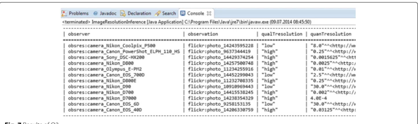
SectionResolution of single observations: Retrieval of Flickr data at a certain temporal resolutionshows how the ODP for the resolution of single sensor observation can be used to annotate and retrieve Flickr data with their tem-poral resolution. The purpose of the section is to illustrate how information from a real dataset could be
accom-modated through the ODP. SectionResolution of single
observations: Expressing resolution qualitatively demon-strates how translation rules in SPARQL can be specified to account for qualitative values of resolution in the con-text of query expansion. Both sections illustrate the use of the ODP for information retrieval and query expan-sion respectively. Since the principles are similar, infor-mation retrieval and query expansion using the ODP for observation collection are not further presented. Instead, SectionResolution of observation collections:

![Fig. 1 Observation process (reprinted from [ 55 ] with permission)](https://thumb-us.123doks.com/thumbv2/123dok_us/7905186.2104642/6.892.89.812.130.302/fig-observation-process-reprinted-permission.webp)