Compositional analysis techniques for multiprocessor soft real-time scheduling

(1)

Compositional Analysis Techniques For Multiprocessor Soft

Real-Time Scheduling

Hennadiy Leontyev

A dissertation submitted to the faculty of the University of North Carolina at Chapel

Hill in partial fulfillment of the requirements for the degree of Doctor of Philosophy in

the Department of Computer Science.

Chapel Hill

2010

Approved by,

Prof. James H. Anderson

Prof. Sanjoy Baruah

Prof. Kevin Jeffay

Prof. Ketan Mayer-Patel

Prof. Jasleen Kaur

(2)

c

2010

(3)

ABSTRACT

HENNADIY LEONTYEV: Compositional Analysis Techniques For Multiprocessor Soft Real-Time Scheduling.

(Under the direction of Prof. James H. Anderson)

The design of systems in which timing constraints must be met (real-time systems) is being affected by three trends in hardware and software development. First, in the past few years, multiprocessor and multicore platforms have become standard in desktop and server systems and continue to expand in the domain of embedded systems. Second, real-time concepts are being applied in the design of general-purpose operating systems (like Linux) and attempts are being made to tailor these systems to support tasks with timing constraints. Third, in many embedded systems, it is now more economical to use a single multiprocessor instead of several uniprocessor elements; this motivates the need to share the increasing processing capacity of multiprocessor platforms among several applications supplied by different vendors and each having different timing constraints in a manner that ensures that these constraints were met. These trends suggest the need for mechanisms that enable real-time tasks to be bundled into multiple components and integrated in larger settings.

There is a substantial body of prior work on the multiprocessor schedulability analysis of real-time systems modeled as periodic and sporadic task systems. Unfortunately, these standard task models can be pessimistic if long chains of dependent tasks are being analyzed. In work that introduces less pessimistic and more sophisticated workload models, only partitioned scheduling is assumed so that each task is statically assigned to some processor. This results in pessimism in the amount of needed processing resources.

(4)

ACKNOWLEDGMENTS

My dissertation and graduate school career would not have been possible without the help of many people. First, I would also like to thank my dissertation committee: James Anderson, Sanjoy Baruah, Kevin Jeffay, Ketan Mayer-Patel, Jasleen Kaur, and Samarjit Chakraborty, for the feedback they have provided during my work. Especially, I am grateful to my advisor, Jim Anderson, who patiently guided me through research and writing over these five years. I cannot imagine a better advisor.

I would also like to thank the UNC Department of Computer Science as a whole for its positive and friendly environment. Due to some great teachers here, I learned more about computer science than I had learned during my previous five years as a student. I owe much to the many colleagues with whom I have published over the years: Uma Devi, Bj¨orn Brandenburg, John Calandrino, Aaron Block. Also, I owe many thanks to my other real-time colleagues: Nathan Fisher and Cong Liu. I wished I had written a paper with you.

I would like to thank people at places where I did my two summer internships in 2007 and 2009: the School of Computing at National University of Singapore and AT&T Labs Research. My collaborator Theodore Johnson at AT&T deserves a large amount of credit for showing that my research can really have a big impact.

Finally, I want to thank my wife. Maria, you are the most wonderful wife I could have asked for. Without you, I would not be able to finish this dissertation and graduate. Thank you for your unconditional love, continuous support, and patience. I love you so much.

(5)

LIST OF TABLES

2.1 System parameters in Example 2.13. . . 41

3.1 χ-values in Example 3.5. . . 46

(9)

LIST OF FIGURES

1.1 Example sporadic task system. . . 6

1.2 SMP architectures. . . 8

1.3 Processor availability restrictions . . . 9

1.4 Multiprocessor PEDF and GEDF schedules. . . 12

1.5 Illustration of limitations of sporadic task model. . . 15

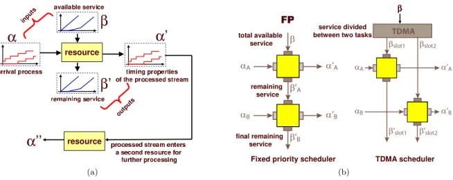
1.6 (a) Computing the timing properties of the processed stream using real-time calculus. (b)Scheduling networks for fixed priority and TDMA schedulers. . . 16

1.7 Complex multiprocessor multimedia application. . . 17

1.8 Example container allocation. . . 21

1.9 Analysis of multiprocessor element using RTC extensions. . . 23

2.1 Example EDZL and EPDF schedules. . . 27

2.2 EPDF schedules with early release . . . 28

2.3 An illustration to SB-test. . . 30

2.4 Example component-based system. . . 32

2.5 Component-based system scheduled using megatasks. . . 33

2.6 Example virtual cluster scheduling. . . 35

2.7 Example of parallel-supply function abstraction. . . 37

2.9 Embedded automotive application. . . 41

3.1 Example priority mappings. . . 45

3.2 Example global LLF schedule. . . 46

3.3 EPDF priority mapping example. . . 47

3.4 Example PS schedule. . . 49

3.6 Job set partitioning. . . 55

3.7 Illustration of proof of Lemma 3.15. . . 62

3.8 Task execution for different processor availability patterns. . . 68

(10)

3.10 Tightness of generalized tardiness bound (I). . . 74

3.11 Tightness of generalized tardiness bound (II). . . 75

4.1 Example container structure. . . 78

4.2 Comparison of supply parallelism. . . 80

4.3 Isolating HRT tasks. . . 82

4.4 Example of processor reclamation. . . 84

4.5 Server task’s minimum and maximum allocation scenarios. . . 91

4.6 Server task allocation and its linear upper bound. . . 93

4.7 Maximum allocation scenario for a HRT task. . . 96

4.8 Illustration of Theorem 4.2. . . 97

4.9 Example of utilization loss in hierarchical scheduling. . . 98

4.10 Container isolation. . . 100

4.11 Experimental setup for hierarchical scheduling. . . 101

4.12 Finding required container bandwidth. . . 103

4.13 Experimental evaluation results. . . 105

5.1 A multiprocessor PE analyzed using multiprocessor real-time calculus. . . 107

5.2 (a)Unavailable time instants and(b)service function in Example 5.4. . . 111

5.3 Conditions for a response-time bound violation forλ= 1. . . 120

5.4 Iterative process for findingδℓin Example 5.9. . . 132

5.5 Conditions for a response-time bound violation forλ= 1. . . 134

5.6 (a)A video-processing application. Experimental setup(b)without and(c)with containers. . 142

5.7 Job arrival curveαuand completion curvesαu′ _{for tasks}_T 1 andT2 in the (a)- and (b)-systems. . 145

(11)

LIST OF ABBREVIATIONS

CA Container-Aware Scheduling EDF Earliest Deadline First EDL Earliest Deadline Last EDZL Earliest Deadline Zero Laxity EPDF Earliest Pseudo-Deadline First FIFO First-In-First-Out

FP Fixed-Priority GEDF Global EDF HRT Hard Real-Time HS Hard-Soft Scheduling LLF Least Laxity First

LLREF Least Local Remaining Execution First NPGEDF Non-preemptive Global EDF

PEDF Partitioned EDF PS Processor-Sharing RM Rate-Monotonic SRT Soft Real-Time

(12)

(13)

Chapter 1 Introduction

The goal of this dissertation is to extend prior work on multiprocessor real-time scheduling to enable soft real-time schedulability theory to meet the expectations of system designers. The particular focus of this work is sets of real-time tasks that need to be integrated as components in larger settings. Such settings include stream-processing (multimedia) applications, systems where computing resources are shared among multiple real-time applications, embedded systems, etc. Prior to the research in this dissertation, scheduling in multiprocessor soft real-time systems has been mainly considered in standalone contexts. In this dissertation, we extend prior work on multiprocessor soft real-time scheduling and construct new analysis tools that can be used to design component-based soft real-time systems. Further, we present novel validation procedures for several well-known scheduling algorithms that allow heterogeneous real-time constraints to be tested in a uniform fashion.

To motivate the need for compositional analysis, we start with a brief introduction to real-time systems. Next, we present the system model that is assumed in this dissertation. We then briefly review prior work on multiprocessor soft real-time scheduling and compositional analysis and state the thesis of this dissertation. Finally, we summarize this dissertation’s contributions and give an outline for the remainder of the dissertation.

1.1 What is a Real-Time System?

(14)

correct-ness. Embedded systems such as automotive controllers and medical devices, some multimedia software, radar signal-processing, and tracking systems are the examples of real-time systems.

Timing constraints are often specified in terms ofdeadlinesfor activities. Based on the cost of failure associated with not meeting them, deadlines in real-time systems can be broadly classified as eitherhard

or soft. A hard real-time deadline is one whose violation can lead to disastrous consequences such as loss of life or a significant loss to property. Industrial process-control systems and robots, controllers for automotive systems, and air-traffic-control systems are some examples of systems with hard deadlines. In contrast, a soft deadline is less critical; hence, soft deadlines can occasionally be violated. However, such violations are not desirable, either, as they may lead to degraded quality of service. For example, in an HDTV player, a new video frame must be created and displayed every 33 milliseconds. If a frame is not processed on time (a deadline is missed), then there may be a perceptible disruption in the displayed video. Another example of a soft real-time application is a real-time data warehouse. Such a system periodically gathers data across a large-scale computer network and analyzes the data in order to identify network performance problems (Golab et al., 2009). As long as most deadlines are met, network problems can be properly detected and handled as they happen. Many multimedia systems and virtual-reality systems also have soft real-time constraints (Block, 2008; Bennett, 2007; Bennett and McMillan, 2005; Vallidis, 2002).

For a real-time system, it should be possible to ensure that all timing requirements can always be met under the assumptions made concerning the system. In other words, the system should bepredictable. Ensuring a priori that timing requirements are met is the core of real-time systems theory and the subject of concentration of this dissertation. In order to make such predictions, for complex real-time systems in which global (resource-efficient) scheduling algorithms are used, appropriate analysis tools are yet to be developed. This motivates the research addressed in this dissertation as explained in the next section in greater detail.

1.2 Motivation

The main goal of this dissertation is to bridge the gap between the current state-of-the-art in multipro-cessor soft real-time scheduling and real-world needs. Such needs are being impacted by three trends in hardware and software development.

(15)

and in-kernel priority-inheritance mechanisms (e.g., the RT-PREEMPT patch for the Linux kernel (RTp, 2009)). This trend has been driven by a growth in applications with timing constraints that developers wish to host on such systems.

Second, new features are being introduced to support “co-hosted” applications. Though general-purpose OSs are typically used to run several applications simultaneously, in some situations, one appli-cation may occupy all available system resources and make the entire system unresponsive. To prevent such behaviors, strong isolation mechanisms known as application containershave been introduced in Linux (LVS, 2007; Eriksson and Palmroos, 2007; Lessard, 2003). Containers are an abstraction that allows different application groups to be isolated from one another (mainly, by providing different name spaces to different application groups for referring to programs, files, etc.). Containers are seen as a lightweight way to achieve many of the benefits provided by virtualization without the expense of run-ning multiple OSs. For example, quotas on various system resources such as processor time, memory size, network bandwidth, etc., can be enforced for encapsulated applications.

Third, these OS-related developments are happening at a time when multicore processors are now in widespread use. Additionally, reasonably-priced “server class” multiprocessors have been available for some time now. One such machine can provide many functions, including soft real-time applications like HDTV streaming and interactive video games, thus serving as amulti-purpose home appliance (In-tel Corporation, 2006). The spectrum of settings where multicore architectures are being used even includes handheld devices. The resulting increase in processing power on such devices enables MPEG video encoding/decoding software to be deployed on them. These hardware-related developments are profound, because they mean that multiprocessors are now a “common-case” platform that software designers must deal with.

(16)

by different vendors. These complicating factors often cause standard workload models and analysis techniques to lead to overly pessimistic results. To enable efficient system design solutions and to reduce design and verification costs, existing compositional frameworks need to be extended so that soft real-time

workloads can be efficiently supported on multiprocessor platforms.

Unlike most prior related efforts (see Chapter 2), we are mainly interested in supporting soft timing constraints. There is growing awareness in the real-time-systems community that, in many settings, soft constraints are far more common than hard constraints (Rajkumar, 2006). If hard constraints do exist, then ensuring themefficientlyon most multiprocessor platforms is problematic for several reasons. First, various processor components such as caches, instruction pipelines, and branch-prediction mechanisms make it virtually impossible to estimate worst-case execution times of programs accurately. (While execution times are needed to analyze soft real-time systems as well, less-accurate empirically-derived costs often suffice in such systems.) Second, while there is much interest in tailoring OSs like Linux to support soft real-time workloads, such OSs are not real-time operating systems and thus cannot be used to support “true” hard timing constraints.

Real-time programs are typically implemented as a collection of threads or tasks. A scheduling algorithm determines which task(s) should be running at any time. A task model describes the pa-rameters of a set of real-time tasks and their timing constraints. On the other hand, a resource model describes the resources available on a hardware platform for executing tasks. The most basic analysis of a real-time system involves running validation tests, which determine whether a real-time system’s timing constraints will be met if a specified scheduling algorithm is used.

In the next section, we describe one of the real-time task models studied in this dissertation. In Sec-tion 1.4, a resource model is presented. In SecSec-tion 1.5, we present some important scheduling algorithms and schedulability tests for them (more algorithms and tests are discussed in detail in Chapter 2).

1.3 Real-Time Task Model

(17)

1.3.1 Sporadic Task Model

Many real-time systems consist of one or more sequential segments of code, calledtasks, each of which is invoked (or released) repeatedly, with each invocation needing to complete within a specified amount of time. Tasks can be invoked in response to events in the external environment that the system interacts with, events in other tasks, or the passage of time as determined by using timers. Each invocation of a task is called ajobof that task, and unless otherwise specified, a task is long-lived, and can be invoked an infinite number of times, i.e., can generate jobs indefinitely.

In this dissertation, we consider a set of n sequential tasks τ ={T1, T2, . . . , Tn}. Associated with each taskTi are three parameters,ei,pi, andDi: ei gives theworst-case execution time(WCET) of any job ofTi, which is the maximum time such a job can execute on a dedicated processor;pi ≥ei, called theperiod ofTi, is the minimum time between consecutive job releases; andDi≥ei, called therelative deadline ofTi, denotes the amount of time within which each job ofTishould complete execution after its release.

Thejth _{job of} _T

i, where j≥1, is denotedTi,j. A task’s first job may be released at any timet≥0. Thearrivalorrelease timeof jobTi,jis denotedri,jand its (absolute) deadlinedi,jis defined asri,j+Di. The completion time ofTi,jis denotedfi,j andfi,j−ri,jis called itsresponse time. TaskTi’s maximum response time is defined as maxj≥1(fi,j−ri,j). The execution time of jobTi,j is denoted ei,j.

For each jobTi,j, we define aneligibility timeǫi,jsuch thatǫi,j≤ri,j andǫi,j−1≤ǫi,j. The eligibility time ofTi,j denotes the earliest time when it may be scheduled. A jobTi,jis said to beearly-released if ǫi,j< ri,j. An unfinished jobTi,j is said to beeligible at timetift≥ǫi,j. The early-release task model was considered in prior work on Pfair scheduling (Anderson and Srinivasan, 2004). As shown later in Example 2.3 in Section 2.1.2, allowing early releases can reduce job response times.

If Di = pi (respectively, Di ≤ pi) holds, then Ti and its jobs are said to haveimplicit deadlines (respectively, constrained deadlines). A sporadic task system in which Di =pi (respectively,Di ≤pi) holds for each task is said to be animplicit-deadline system(respectively,constrained-deadline system). In anarbitrary-deadline system, there are no constraints on relative deadlines and periods. For brevity, we often use the notationTi(ei, pi, Di) to specify task parameters in constrained- and arbitrary-deadline systems andTi(ei, pi) in implicit-deadline systems.

(18)

t

0 2 4 6 8 10 12

T

3,1

T

3,2

T

1,1

T

1,2

T

2,2

T

2,1

T

2,3

T

3,1

t

0 2 4 6 8 10 12

T

3,1

T

3,2

T

1,1

T

1,2

T

2,2

T

2,1

T

2,3

T

3,1

job release job deadline job eligibility time

(a) (b)

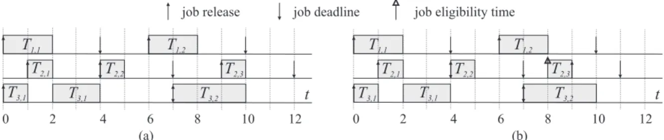
Figure 1.1: Example schedules of a sporadic task system from Example 1.1.

max(0, fi,j−di,j), and thetardinessof taskTiin scheduleSis defined astardiness(Ti,S) = maxj≥1(tardiness(Ti,j,S)). Because Ti is sequential, its jobs may not execute on multiple processors at the same time, i.e.,

parallelism is forbidden even if deadlines are missed. Further, a tardy job does not delay the releases of later jobs of the same task.

A task with the characteristics as described is referred to as a sporadic task and a task system composed of sporadic tasks is referred to as a sporadic task system. Aperiodic taskTi is a special case of a sporadic task in which consecutive job releases are separated by exactly pi time units, and a task system whose tasks are all periodic is referred to as a periodic task system. A periodic task system is calledsynchronousif all tasks release their first jobs at the same time, andasynchronous, otherwise.

Example 1.1. An example sporadic task system with two implicit-deadline sporadic tasksT1(2,4) and T2(1,3) and one periodic taskT3(3,7) running on two processors is shown in Figure 1.1(a). Figure 1.1(b) shows the same task system except that job T2,3 is released early by one time unit. In this example, we assume that jobs ofT1have higher priority than those of T2 andT3. In the rest of the dissertation, up-arrows will denote job releases and down-arrows will denote job deadlines (if any).

Definition 1.1. Theutilization of sporadic taskTi is defined as ui=ei/pi, and the utilization of the task system τ asUsum(τ) =PTi∈τui.

The utilization ofTiis the maximum fraction of time on a dedicated processor that can be consumed byTi’s jobs over an interval during which a large number ofTi’s jobs are released. In Example 1.1, task T1can consume up to half of the available processing time on a dedicated processor.

1.3.2 Hard vs. Soft Timing Constraints

(19)

Alternatively, if, for task Ti, deadline misses are allowed, then Ti is called a soft real-time (Soft Real-Time (SRT))task. The system containing one or more SRT tasks is called asoft real-time(SRT)

system. Because jobs in SRT systems may miss deadlines occasionally, there is no single notion of SRT correctness. Some possible notions of SRT correctness include: bounded deadline tardiness (i.e., each job completes within some bounded time after its deadline) (Devi, 2006); a specified percentage of deadlines must be met (Atlas and Bestavros, 1998); and m out of every k consecutive jobs of each task complete before their deadlines (Hamdaoui and Ramanathan, 1995). In this dissertation, we are primarily concerned with HRT systems and SRT systems with bounded deadline tardiness. Bounded tardiness is important because each task with bounded tardiness can be guaranteed in the long run to receive processor time proportional to its utilization.

With HRT and SRT correctness defined as above, HRT correctness is simply a special case of SRT correctness. In both cases, we are concerned with whether a task’s response time occurs within a specified bound. If a task’s maximum response time is required to be at most its relative deadline, then that task is a HRT task. If it is required to be at most the relative deadline plus the maximum allowed tardiness, then that task is a SRT task.

In Chapters 3 and 4, we will specify timing requirements in terms of deadlines and tardiness. In Chapter 5, we will specify timing constraints in terms of maximum response times.

1.4 Resource Model

In this dissertation, we consider real-time task systems running on a platform comprised of a set of m ≥2 identical unit-speed processors. Such a platform is called an identical multiprocessor platform. In this setting, all processors have the same characteristics, including uniform access times (in the absence of contention) to memory. Later, in Chapter 3, we also discuss how some of the results of this dissertation can be applied touniform multiprocessorplatforms, in which processors can have different speeds, i.e., different processors may execute instructions at different rates. Unless stated otherwise, in this dissertation, we assume that the platform is an identical multiprocessor.

(20)

CPU1

cache L1, L2,...

CPU2

cache L1, L2,...

CPU3

cache L1, L2,...

Memory bus interconnect

Memory

(a)

CPU1

L1

CPU2 CPU3

Memory bus interconnect

Memory

L1 L1

Shared L2 cache

(b)

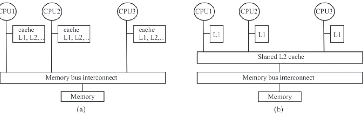
Figure 1.2: Symmetric multiprocessor architecture(a)without and(b)with a shared cache.

job (task) executes on different processors at different times, then we say that that job (task)migrates. When a job migrates, it may be necessary to load task-related instructions and data into a local cache. One of the ways to lower migration overheads is to restrict the execution of a task or a job to one or a subset of processors. Another way is to use a multicore architecture with shared caches. As the name suggests, the multicore chip has several processing cores on one die, which reduces power consumption and production costs. In addition, different cores may share a cache at some level as illustrated in Figure 1.2(b). Shared caches may reduce migration overheads, if task-related data and instructions do not need to be loaded from memory after a migration. Task preemptions, context switches, task migrations, and scheduler activity are system overheads that take processor time from the task system. It is not possible to predict the behavior of the system without accounting for these overheads. This problem is exacerbated in a platform with shared caches: due to cache interference, each individual job’s execution time will depend on the job set being currently scheduled. Commonly, overheads are accounted for by charging each external activity (e.g., a preemption, migration, or scheduler invocation) to a unique job, and the WCET of each task is inflated by the maximum cumulative time required for all the external activities charged to any of its jobs. Throughout this dissertation, we will assume that system overheads are included in the WCETs of tasks using efficient charging methods (Devi, 2006). The WCET of a task is therefore dependent on the implementation platform, application characteristics, and the scheduling algorithm.

(21)

t

0 2 4 6 8 10 12

p

1

(a)

0 2 4 6 8 10 12

0 1 2 3 4 5

b (D)*

D

b (D)=l D

1 max(0,5/8( -2))

(b)

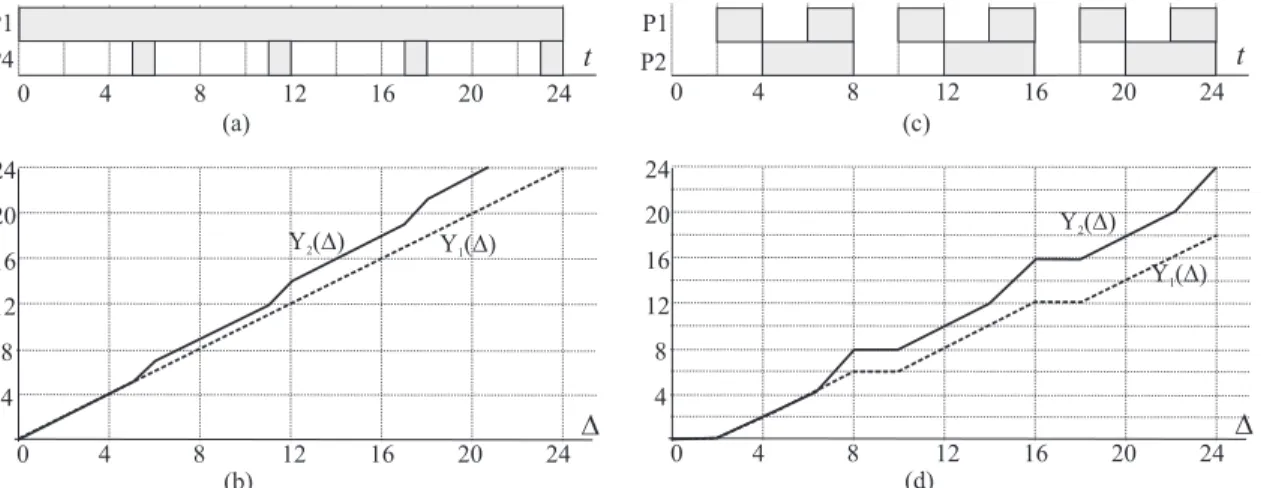
Figure 1.3: (a) Unavailable time instants and (b) service functions for processor 1 (denoted P1) in Example 1.2.

Definition 1.2. The minimum guaranteed time that processorhcan provide toτ in any time interval of length ∆≥0 is characterized by the service function

βhl(∆) = max(0,cuh·(∆−σh)), (1.1)

whereu_ch∈(0,1] andσh≥0.

In the above definition,uch is the total long-term utilization available to the tasks inτ on processor h and σh is the maximum length of time when the processor can be unavailable. These parameters are similar to those in the bounded delay model (Mok et al., 2001) and multi-supply function abstrac-tion (Bini et al., 2009b). We require_cuh(∆) andσh to be specified for eachh. Note that, if (unit-speed) processorhis fully available to the tasks inτ, thenβl

h(∆) = ∆.

Example 1.2. Consider a system with a processor that is not fully available. The availability pattern, which repeats every eight time units, is shown in Figure 1.3(a); intervals of unavailability are shown as black regions. For processor 1, the minimum amount of time that is guaranteed toτ over any interval of length ∆ is zero if ∆≤2, ∆−2 if 2≤∆≤4, and so on. Figure 1.3(b) shows the minimum amount of time β∗_{(∆) that is available on processor 1 for soft real-time tasks over any interval of length ∆. It}

also shows a service curveβ1(∆) = max(0,cu1(∆−σ1)), wherecu1=5₈ andσ1= 2, which boundsβ∗(∆) from below. β1(∆) can be used to reflect the minimum service guarantee for processor 1.

(22)

1.5 Real-Time Scheduling Algorithms and Tests

The ultimate goal of real-time systems analysis is guaranteeing temporal correctness. That is verifyinga priorithat no job deadline is ever missed or, if deadlines are allowed to be missed, then these misses are by no more than certain amount of time. Temporal correctness depends on how jobs are scheduled. A

scheduling algorithmis used at runtime to determine which job to run next on the available processors.

Definition 1.3. A task system τ is concrete if the release and eligibility times of all of its jobs are specified and isnon-concreteotherwise.

The task set considered in Example 1.1 is a non-concrete task system, while the schedules considered in this example are produced by two concrete instantiations ofτ with different eligibility times forT2,3. In the real-time systems literature, a concrete task system τ isfeasible on a given platform if there exists a schedule in which no job deadline is missed. A non-concrete task systemτ is feasible on a given platform if every concrete instantiation ofτ is feasible.

A HRT systemτis calledschedulableunder scheduling algorithmAon a given platform if no deadline is missed in the schedule produced byAfor any concrete instantiation ofτ. Alternatively, a SRT system τis schedulable underAif the maximum task tardiness is bounded. Often, tardiness bounds arespecified

by system designers. Let Θi be the maximum allowed tardiness for task Ti. (Note that if Θi = 0 for each taskTi, then the system is HRT.) In this case,τ is schedulable if these specified tardiness bounds are not exceeded.

Associated with a scheduling algorithm is a procedure for verifying schedulability called a schedula-bility test. In the rest of the section, we briefly describe the earliest-deadline-first (Earliest Deadline First (EDF)) scheduling algorithm for uniprocessor and multiprocessor platforms and schedulability results for it when considering implicit-deadline task systems. Other important scheduling algorithms, their associated schedulability tests, and schedulability tests for EDF for constrained- and arbitrary-deadline sporadic task systems are discussed in detail in Chapter 2. In the discussion below, we assume that all processors are fully available.

1.5.1 Uniprocessor Scheduling

(23)

For an implicit-deadline task systemτ, all deadlines can be met iffUsum(τ)≤1 (Liu and Layland,

1973). In contrast, if Usum(τ)>1, then some tasks inτ have unbounded deadline tardiness in certain

concrete instantiations of τ (e.g., when job releases are periodic). Therefore, the notions of HRT and SRT schedulability are the same for implicit-deadline systems under uniprocessor EDF.

1.5.2 Partitioned Multiprocessor Scheduling

Similarly to uniprocessor scheduling, under multiprocessor scheduling, an implicit-deadline task system τ isfeasible onmprocessors iff Usum(τ)≤m (Anderson and Srinivasan, 2000; Baruah et al., 1996). If

τ is schedulable using an algorithmAonm′ _{processors, then the difference}_m′₋_U

sum(τ) is called the utilization loss. We would like to minimize such loss while still be able to satisfy all timing requirements. Most multiprocessor scheduling algorithms can be classified as either partitioned or global (or some combination thereof). Inpartitionedalgorithms, each task is permanently assigned to a specific processor and each processor independently schedules its assigned tasks using a uniprocessor scheduling algorithm. Inglobalscheduling algorithms, tasks are scheduled from a single priority queue and may migrate among processors.

The advantage of partitioned schedulers is that they enable uniprocessor schedulers to be used (on each processor) and usually have low migration/preemption costs. The disadvantage of partitioned schedulers is that they may require more processors to schedule a task system when compared to global schedulers (as we will see later in this section). In this section, we consider the partitioned EDF (Parti-tioned EDF (PEDF)) scheduling algorithm.

Because uniprocessor EDF is optimal, for implicit-deadline task systems, it suffices to construct a partition of τ into the m subsets {τk} such that, for each k, Usum(τk) ≤ 1. This partitioning prob-lem is related to the NP-complete bin-packing probprob-lem and becomes even more difficult for restricted-and arbitrary-deadline systems. For these task systems, some sufficient schedulability tests have been developed for partitioned EDF and static-priority scheduling (Baruah and Fisher, 2006, 2007). Unfor-tunately, not all task sets can be successfully partitioned. In general, an implicit-deadline task system τ with utilizationUsum(τ) could require up to ⌈2·Usum(τ)−1⌉processors in order to be schedulable

(24)

t

0 2 4 6 8 10 12

T

3,1

T

1,1

T

1,2

T

2,2

T

2,1

T

1,3

T

3,2

P1 P2

T

4,1

T

4,1

(a)

t

0 2 4 6 8 10 12

T

3,1

T

1,1

T

1,2

T

2,2

T

2,1

T

1,3

T

1,4

T

3,2

P1 P2 P3

T

4,1

T

4,2

(b)

t

0 2 4 6 8 10 12

T

3,1

T

4,1

T

1,1

T

1,2

T

2,2

T

2,1

T

1,3

T

1,4

T

3,2 P1 P2

T

4,2

T

4,1 (c)

t

0 2 4 6 8 10 12

T

3,1

T

4,1

T

1,1

T

1,2

T

2,2

T

2,1

T

1,3

T

1,4

T

3,2

P1 P2

T

4,2

(d)

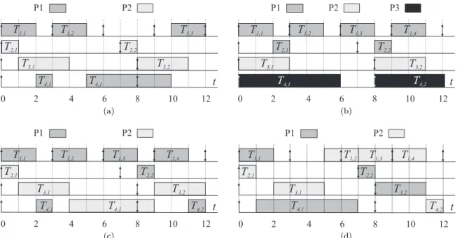
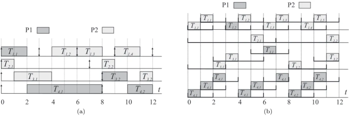
Figure 1.4: (a)Two- and(b)three-processor PEDF schedules in Example 1.3. (c)Preemptive and(d) nonpreemptive GEDF schedules in Example 1.4.

Example 1.3. Consider an implicit-deadline task system τ = {T1(2,3), T2(1,7), T3(3,8), T4(6,8)}, which has total utilization Usum(τ) ≈ 1.93 ≤ 2. As mentioned at the beginning of Section 1.5.2, τ

is feasible on two processors. For any partitioning of this task set onto two processors, the total utiliza-tion of the tasks assigned to one of the processors is greater than one. Therefore,τ cannot be scheduled under PEDF on two processors so that all tasks meet their deadlines (or have bounded deadline tardi-ness).

(25)

1.5.3 Global Multiprocessor Scheduling

In contrast to partitioned scheduling, some global schedulers incur no utilization loss in implicit-deadline systems. Global algorithms can be further classified as either restricted or unrestricted. A scheduling algorithm is considered to be restricted if the scheduling priority of each job (for any given schedule) does not change once the job has been released. A scheduling algorithm is considered to beunrestricted

if there exists a schedule in which some job changes its priority after it is released.

In this section, we discuss two restricted global scheduling algorithms, preemptive global EDF (Global EDF (GEDF)) and non-preemptive global EDF (Non-preemptive Global EDF (NPGEDF)); unrestricted algorithms are considered later in Section 2.1.2. Under both GEDF and NPGEDF, tasks are scheduled from a single priority queue on an EDF basis. The only difference between GEDF and NPGEDF is that jobs can be preempted under GEDF and cannot be preempted under NPGEDF.

Example 1.4. Consider the task systemτ from Example 1.3. An example GEDF schedule for τ on two processors is shown in Figure 1.4(c). In this schedule, job T4,1 misses its deadline at time 8 by one time unit. Note that, in this schedule, taskT4 migrates between processors 1 and 2. Figure 1.4(d) shows a NPGEDF schedule forτ. In this schedule, jobT4,1 meets its deadline. However, jobT1,2misses its deadline by one time unit because it is blocked by lower-priority jobs of T3 andT4 during the time interval [3,5).

Similarly to PEDF, GEDF may leave up to half of the system’s processing capacity unused if HRT schedulability is required. Particularly, an implicit-deadline sporadic task system τ with total utiliza-tion Usum(τ) and max(ui) ≤ 1/2 may need up to ⌈2·Usum(τ)−1⌉ processors in order to be HRT

schedulable (Baruah, 2003). (Even more processors may be needed if max(ui)>1/2.)

In contrast, for purely SRT systems, utilization loss can be eliminated. According to Devi and Anderson (2008b), for an implicit-deadline task system τ, bounded deadline tardiness is guaranteed under GEDF and NPGEDF if Usum(τ) ≤ m. For the task system τ in Example 1.4, the maximum

deadline tardiness is at most 8.5 under GEDF (see Section 2.1.1 for details).

We conclude this section by briefly mentioning one unrestricted global scheduler, namely, thePD2 Pfair algorithm, which is one of the few optimal multiprocessor scheduling algorithms for implicit-deadline task systems. Any such task systemτ, where tasks have integral execution times and periods and Usum(τ)≤m, is HRT schedulable byPD2(Anderson and Srinivasan, 2004). Conversely, ifUsum(τ)> m,

(26)

schedulers are discussed in greater detail later in Section 2.1.2.

1.6 Limitations of the Sporadic Task Model

Modern embedded systems are becoming complex and distributed in nature. Such complexity may preclude efficient analysis using the periodic and sporadic models, thus making the schedulability results described in the prior sections inapplicable.

In this section, we use an example to illustrate some of the critical limitations of the sporadic task model that can arise during the analysis of a real application. We then briefly describe the streaming task model and the associated real-time calculus analysis framework, which circumvents these limitations and is widely used in the analysis of embedded systems.

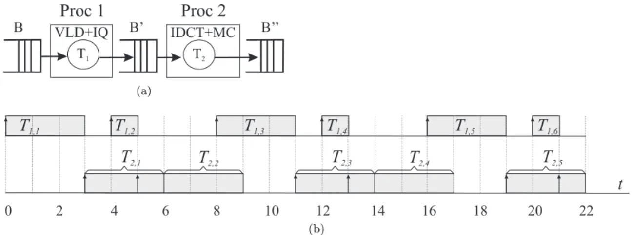
Example 1.5. We consider an MPEG-2 video decoder application that has been studied previously in (Chakraborty et al., 2006; Phan et al., 2008). The originally-studied application, shown in Fig-ure 1.5(a), is partitioned and mapped onto two processors. Processor 1 runs the VLD (variable-length decoding) and IQ (inverse quantization) tasks, while processor 2 runs the IDCT (inverse discrete cosine transform) and MC (motion compensation) tasks. The (coded) input bit stream enters this system and is stored in the input buffer B. The macroblocks (portions of frames of size 16×16 pixels) in B are first processed by taskT1 and the corresponding partially-decoded macroblocks are stored in the buffer B′ _{before being processed by} _T

2. The resulting stream of fully decoded macroblocks is written into a playout buffer B′′ _{prior to transmission by the output video device. In the above system, the coded}

input event stream arrives at a constant bit-rate.

(27)

IDCT+MC

Proc 1

Proc 2

B

T2

B’ B’’

VLD+IQ T1

(a)

t

0 2 4 6 8 10 12 14 16 18 20 22

T

1,1

T

1,2

T

2,2

T

2,4

T

2,1

T

2,3

T

2,5

T

1,3

T

1,4

T

1,5

T

1,6

(b)

Figure 1.5: (a)MPEG Player application and(b)example schedule of tasksT1andT2in Example 1.5.

is u1 = 0.75. However, task T1’s effective utilization is 0.5 as it consumes half of the capacity of one processor over sufficiently long time intervals.

In the example above, the sporadic task model is insufficient because it does not capture the long-term execution requirements of tasks or long-long-term job arrival patterns. The multiframe and periodic with jitter task models have been proposed to include these features in task descriptions (Mok and Chen, 1997). However, a more systematic approach to the analysis of communicating tasks such as those in Example 1.5 was enabled with the introduction of the streaming task modeland the real-time calculusframework described next (Chakraborty et al., 2003, 2006).

1.7 Real-Time Calculus Overview

(28)

us-(a) (b)

Figure 1.6: (a) Computing the timing properties of the processed stream using real-time calculus. (b)Scheduling networks for fixed priority and TDMA schedulers.

ing functionsβu_{(∆) and} _βl_{(∆), which specify the maximum and minimum number of serviced events,} respectively, within any interval of length ∆. Given the functions αu(∆) and αl(∆) corresponding to an event stream arriving at a resource, and the serviceβu(∆) and βl(∆) offered by it, it is possible to compute the timing properties of the processed stream and remaining processing capacity, i.e., functions αu′_(∆), _αl′_(∆), _βu′_{(∆), and} _βl′_{(∆), as illustrated in Figure 1.6(a), as well as the maximum backlog} and delay experienced by the stream. As shown in the same figure, the computed functions αu′_(∆)

andαl′_{(∆) can then serve as inputs to the next resource on which this stream is further processed. By} repeating this procedure until all resources in the system have been considered, timing properties of the fully-processed stream can be determined, as well as the end-to-end event delay and total backlog. This forms the basis for composing the analysis for individual resources, to derive timing/performance results for the full system.

(29)

Proc 1

Proc 3

Proc 5

Proc 7

S1

S2

S3

S4

T2

T4

T6

T8

Proc 2

Proc 4

Proc 6

Proc 8

T1

T3

T5

T7

Three processors

T3 T4

T7 T8

U=1.4 U=1.4

T1 T2

C2

C3 C4

T5 T6

(a) (b)

S1

S2

S3

S4

C1

Figure 1.7: A complex multiprocessor multimedia application under (a) partitioning and (b) global scheduling.

analyzing distributed real-time systems.

1.8 Research Needed

With the needed background and concepts in place, we return to the subject of this dissertation, namely, extending compositional techniques for the design and analysis of real-time systems on multiprocessors. We motivate the open research questions in this area by looking at an example real-time multimedia system.

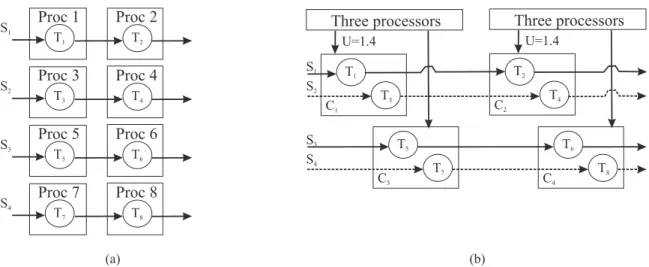
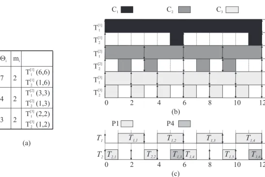
Consider an application consisting of four MPEG decoders similar to that in Figure 1.5(a) that process four video streams S1, . . . , S4 as shown in Figure 1.7(a). Tasks T1 and T2 process stream S1, tasks T3 and T4 process stream S2, and so on. Suppose that each task requires 70% of the capacity of a dedicated processor. If partitioning is used, then the entire application requires eight processors to accommodate all tasks. However, since the cumulative utilization requirement is 0.7·8 = 5.6, six processors may be sufficient if global scheduling is used. Additionally, suppose that we want to isolate the tasks processing different groups of streams into containers as shown in Figure 1.7(b). Here, the tasks are encapsulated into four containersC1, . . . , C4. Containers C1 and C3 are scheduled using the first three processors and containersC2andC4are scheduled using the remaining three processors. Such a setup would ensure isolation between two groups of streams if some tasks request more resources than provisioned.

(30)

first note that, since each task has a utilization of 70%, each container has a utilization of 140%, which requires the capacity of more than one processor. This poses the first problem.

(i) How can the processing capacity of a multiprocessor platform be allocated to a set of containers some of which require more than one processor? How can the supply available to each of the containers be characterized?

One potential solution, which is described and analyzed formally in Chapter 4, is to fully dedicate processor 1 and 40% of the capacity of processor 2 to running tasks in C1. The remaining time on processors 2 and 3 can be used for running tasks in C3. Containers C2 and C4 can be dealt with similarly.

Given a characterization of the supply for each container, tasks can be viewed as being scheduled on a set of partially-available processors. The problem of verifying timing constraints on a restricted-capacity platform has received some recent attention. However, these efforts only consider sporadic tasks with HRT constraints (Bini et al., 2009b; Anderson et al., 2006; Easwaran et al., 2009). We review this prior work in greater detail in Chapter 2. Allowing timing constraints to be soft for some tasks poses the second research problem.

(ii) Which scheduling algorithms can ensure SRT constraints (e.g., bounded tardiness or bounded maximum task response times) for workloads scheduled on a set of partially-available processors? Which such algorithms require the least processor supply?

Finally, we need to calculate the timing properties of the fully-processed streams, as well as the end-to-end event delay and total backlog. This poses the third research problem.

(iii) How can the properties mentioned above be analyzed for a set of streaming tasks scheduled using a global scheduler on a set of partially-available processors?

1.9 Thesis Statement

The main thesis of this dissertation, which attempts to answer the three research questions above, is the following.

With the exception of static-priority algorithms, virtually all previously studied global real-time scheduling

algorithms ensure bounded deadline tardiness for implicit-deadline sporadic task systems. This property

(31)

long-term execution demand does not exceed the total available processing capacity. Well-studied global

schedulers such as GEDF and First-In-First-Out(First-In-First-Out (FIFO))ensure bounded maximum response times in systems with complex job arrival and execution patterns as described by the streaming

task model. The use of such algorithms enables component-based systems with predominantly soft timing

constraints to be built while incurring little or no utilization loss in settings where partitioning approaches

are too costly in terms of needed processing resources.

1.10 Contributions

In this section, we briefly describe the contributions of this dissertation.

1.10.1 Generalized Tardiness Bounds

The first contribution we discuss is a generalized job prioritization rule originally proposed in (Leontyev and Anderson, 2008a, 2010) and tardiness bounds under it.

We found that the singular characteristic needed for tardiness to be bounded under a global scheduling algorithm is that a pending job’s priority eventually (in bounded time) is higher than that of any future job. Global algorithms that donot have this characteristic (and for which tardiness can be unbounded) include static-priority algorithms such as the rate-monotonic (Rate-Monotonic (RM)) algorithm, and impractical dynamic-priority algorithms such as the earliest-deadline-last(Earliest Deadline Last (EDL)) algorithm, wherein jobs with earlier deadlines havelower priority. Global algorithms thatdo have this property include the EDF, FIFO, EDF-until-zero-laxity (Earliest Deadline Zero Laxity (EDZL)), and least-laxity-first (Least Laxity First (LLF)) algorithms. (EDZL is described later in Section 2.1.2 and LLF is described in Section 3.2.)

(32)

Pseudo-Deadline First (EPDF)) Pfair algorithm, so these algorithms have bounded tardiness. (For EDF, EPDF, and PD2, this was previously known.) For any other algorithm that may be devised in the future, our results enable tardiness bounds to be established by simply showing that prioritizations can be expressed in a window-constrained way (instead of laboriously devising a new proof).

The notion of a window-constrained priority is very general. For example, it is possible to describe hybrid scheduling policies by combining different prioritizations,e.g., using a combination of EDF and FIFO in the same system. Priority rules can even change dynamically (subject to the window con-straint). For example, if a task has missed too many deadlines, then its job priorities can be boosted for some time so that it receives special treatment. Or, if a single job is in danger of being tardy, then its prioritization may be changed so that it completes execution non-preemptively (provided certain re-strictions hold — see Section 3.4.5). Tardiness also remains bounded if early-release behavior is allowed or if the capacity of each processor that is available to the (soft) real-time workload is restricted. In simplest terms, the main message is that,for global scheduling algorithms, bounded tardiness is the com-mon case, rather than the exception(at least, ignoring clearly impractical algorithms such as EDL). For the widely-studied EDZL and LLF algorithms, and for several of the variants of existing algorithms just discussed, this dissertation is the first to show that tardiness is bounded. The proposed formulation of job priorities has been used by other researchers for the design and implementation of cache-aware mul-tiprocessor real-time schedulers (Calandrino, 2009) and for devising new interrupt accounting techniques on multiprocessors (Brandenburg et al., 2009).

1.10.2 Processor Bandwidth Reservation Scheme

The second major contribution of this dissertation is a new multiprocessor scheduling approach for multi-level hierarchical containers that encapsulate sporadic SRT and HRT tasks. In this scheme, each container is allocated a specifiedbandwidth, which it uses to schedule its children (some of which may also be containers).

(33)

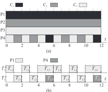
job release job deadline C1 C3

0 2 4 6 8 10 12 14 16 18 20 22 24 26 28 30 32 34 t P1

P2

P3

S3,1 S1,1 S3,2 S1,2 S3,3 S1,3 S3,4

Figure 1.8: Illustration to container allocation in Example 1.6.

Second, each child containerCj is given⌊w(Cj)⌋dedicated processors from the set of⌊w(H)⌋processors dedicated toH. Third, for each child containerCjwith a non-integral bandwidth, aserver taskSj(ej, pj) is created such thatuj = w(Cj)− ⌊w(Cj)⌋. When task Sj is scheduled, tasks fromCj are scheduled. The set of SRT tasks and server tasks is scheduled together on processors that are not reserved for HRT tasks and child containers using an algorithm that ensures bounded tardiness for each task. Each child containerCj thus receives processing time approximately proportional to its requested bandwidth. Applying this strategy recursively, we can accommodate an entire container hierarchy.

Example 1.6. Consider the multimedia application introduced in Section 1.8. We define the bandwidth of container C1 and C3 to be w(C1) =w(C3) = 1.4. Since the bandwidth is non-integral, for each of the containers C1 andC3 we dedicate ⌊w(C1)⌋=⌊w(C3)⌋= 1 processor and construct periodic server tasks S1(4,10) and S3(4,10) with utilizations u1 = u3 = 0.4. Figure 1.8 shows an example schedule in which processors 1 and 3 are dedicated to containersC1 andC3 and the server tasks are scheduled using EDF on processor 2. Each container thus receives the capacity of approximately 1.4 processors over sufficiently long time intervals.

Our scheme is novel in that, in a system with only SRT tasks, no utilization loss is incurred (assuming that system overheads are negligible—such overheads will cause some loss in any scheme in practice). This statement is true, provided the goal is to schedule SRT tasks so that their tardiness is bounded, no matter how great the bound may be. The scheduling scheme we present also allows HRT tasks to be supported. However, such support may incur some utilization loss. These tradeoffs are discussed in detail in Section 4.5.

(34)

1.10.3 Multiprocessor Extensions to Real-Time Calculus

The third major contribution is a framework for the analysis of multiprocessor processing elements with streaming tasks where the constituent processors are managed according to a global multiproces-sor scheduling algorithm. Such processing elements can be used for building complex applications that cannot be analyzed using state-of-the-art multiprocessor scheduling techniques and that must be over-provisioned, wasting processing resources, if analyzed using conventional real-time calculus. Sporadic and streaming task sets under GEDF, and static-priority schedulers, can be analyzed in this framework. Our work is different from prior efforts that assume implicit deadlines, full processor availability, and non-zero tardiness for each task (Devi, 2006; Devi and Anderson, 2005, 2006). In one recent paper, Bini et al. (2009a) presented a HRT schedulability test for GEDF for systems where processors can be partially available. However their work also assumes that tasks are sporadic and have constrained deadlines. In contrast, the task model and the scheduler assumed in our proposed framework are very general.

The core of our framework is a procedure for checking that arbitrary pre-defined job response times

{Θ1, . . . ,Θn}are not violated under a restricted global scheduling algorithm on a platform with a min-imum cumulative capacityB(∆). Note that, if relative deadlines and tardiness thresholds are specified for tasks, then checking pre-defined job response times is equivalent to checking whether a job completes within its relative deadline plus its tardiness threshold.

In settings where response-time bounds{Θ1, . . . ,Θn}are not known, they must be determined. In ad-dition to giving a test that checks pre-defined response-time bounds, we propose closed-form expressions for calculating response-time bounds directly from task and supply parameters for a family GEDF-like schedulers such as GEDF and FIFO. The obtained expressions for response-time bounds are similar to those for calculating tardiness bounds under GEDF proposed by Devi and Anderson (2008b). It is also possible to refine the obtained response-time bounds by incrementally decreasing them and running the aforementioned test procedure to see if the smaller bounds are also valid.

Once maximum job response-time bounds{Θ1, . . . ,Θn}are determined, we use them to characterize the sequences of job completion events for each taskTi in terms of arrival functionsαui

′_{(∆) and}_αl i

′

(∆), and the remaining cumulative processor supplyB′_{(∆) (see Figure 1.9). The calculated stream and supply}

(35)

a

1

a

’

1

a

’’

1

B

’

a

n

a

’

n

Response-time calculation

Q1

Qn

{Q1,...,Qn}

Supply output calculation

Stream output calculation

Figure 1.9: A multiprocessor element analyzed using multiprocessor real-time calculus.

1.11 Summary

In this chapter, we have motivated the research in this dissertation with the need to support component-based systems on multiprocessor platforms. We have presented the widely-studied sporadic task model and some important multiprocessor scheduling algorithms for it. We have also shown that this model may be insufficient for describing workloads in component-based systems. After stating several open research questions pertaining the design and analysis of multiprocessor component-based systems, we gave a list of contributions of this dissertation addressing these questions.

(36)

Chapter 2 Prior Work

In this chapter, we review prior work that is relevant to the focus of this dissertation on multiprocessor schedulability analysis, hierarchical scheduling, and real-time calculus. In Section 2.1, we present some schedulability results for implicit-deadline task systems under GEDF and NPGEDF and illustrate other important multiprocessor scheduling algorithms. In Section 2.2, we review two recent approaches for checking the schedulability of constrained-deadline task systems on fully-available multiprocessor platforms by Baruah (2007) and Bertogna et al. (2008). In this dissertation, we extend the techniques proposed by Baruah by incorporating more expressive task and processor supply models. However, we adopt some ideas from Bertogna et al. as well. In Section 2.3, we present three multiprocessor hierarchical scheduling frameworks for HRT and SRT tasks. One of these frameworks, proposed by Bini et al. (2009a), is based upon the test by Bertogna et al. Another one, proposed by Easwaran et al. (2009), is based upon Baruah’s test. In addition to presenting the ideas behind these frameworks, we also compare them to the hierarchical scheduling scheme proposed in this dissertation. Finally, in Section 2.4, we review prior work on real-time calculus.

2.1 Multiprocessor Scheduling

In this section, we discuss some results concerning HRT and SRT schedulability of implicit-deadline sporadic task systems under GEDF, and present several unrestricted global multiprocessor schedulers.

2.1.1 GEDF Schedulability Results

(37)

schedulability tests (Baker, 2003; Baruah, 2007; Baruah and Baker, 2008; Bertogna et al., 2008). If such a test passes, then each task is guaranteed zero tardiness. Unfortunately, ensuring zero tardiness under GEDF may severely restrict system utilization. According to Goossens et al. (2003), an implicit-deadline task systemτ can be guaranteed to meet all deadlines onmprocessors under GEDF if

m≥

_U

sum(τ)−1 1−max(ui)

.

The task set from Example 1.3 in Section 1.5.3 may thus require m ≥ lUsum(τ)−1

1−max(ui)

m

= l1.93₁₋_3/4−1m =

⌈3.72⌉= 4 processors in order to meet all job deadlines. Because the total utilization isUsum(τ)≈1.93,

half of the platform’s processing capacity will be unused in this case.

As mentioned earlier in Section 1.5.3, Devi and Anderson (2008b) showed that, for an implicit-deadline task systemτ, bounded deadline tardiness is guaranteed under GEDF and NPGEDF ifUsum(τ)≤

m. That is, for SRT systems, utilization loss can be eliminated. Let

λ=

      

Usum−1 ifUsum is integral,

⌊Usum⌋ otherwise.

Then deadline tardiness for taskTi under GEDF is at most

ei+EL

−min(ei)

m−UL , (2.1)

where EL is the sum of λ largest task WCETs and UL is the sum of λ−1 largest task utilizations. Similar expression were obtained in (Devi and Anderson, 2008b) for NPGEDF and for the case when tasks consist of interleaving preemptive and non-preemptive regions. If tardiness thresholds Θi are specified, then we can calculate tardiness bounds Θ′

i using (2.1) and then verify that Θ′i ≤ Θi holds for each task Ti. Unfortunately, this method cannot be applied if some tardiness thresholds are small because Θ′

i ≥ ei for each Ti ∈ τ. This precludes the analysis of systems with mixed HRT and SRT constraints. Also, (2.1) is applicable only to implicit-deadline task systems.

(38)

One can argue that in order to verify pre-defined tardiness thresholds, taskTi’s relative deadline can be set toDi+ Θi, whereDi is the old relative deadline and Θi isTi’s allowed tardiness threshold, and then the HRT schedulability of the modified system can be verified. Though this method is valid for the verification of timing constraints, it changes the relative priority of jobs of different tasks, which may be unacceptable.

Additionally, introducing tardiness thresholds allows a job’s timing constraint to be decoupled from its scheduling priority. For example, an arbitrary-deadline task systemτwith relative deadlines{D1, . . . , Dn} that is not HRT schedulable under GEDF can be SRT schedulable for a different set of relative deadlines

{D′1, . . . , Dn′} and tardiness thresholds {Θ′1, . . . ,Θ′n} such that Di′+ Θ′i = Di for each i. The idea of decoupling priorities and timing constraints is elaborated on in greater detail in Chapter 3.

2.1.2 Unrestricted Global Multiprocessor Scheduling

Unrestricted schedulers allow job priorities to change at runtime. In this section, we briefly present the earliest-deadline-zero-laxity (EDZL), earliest-pseudo-deadline-first (EPDF), PfairPD2_{, and} least-local-remaining-execution-first (Least Local Remaining Execution First (LLREF)) algorithms.

EDZL algorithm. EDZL, which was first proposed by Cho et al. (2002), is a conventional GEDF algorithm with an added “safety rule.” Under EDZL, a job is prioritized by its deadline unless it is in danger of missing its deadline. This moment is detected by calculating the job’s laxity, which is the difference between the current time and the latest time when the job can be scheduled so that it meets its deadline. Jobs with zero laxity are given the highest priority.

Example 2.1. Consider the task set from Example 1.4. An example EDZL schedule for it is shown in Figure 2.1(a). In this schedule, at time 0, all jobs have positive laxity (i.e., if scheduled immediately, each job will complete before its deadline). Therefore, jobs T1,1 and T2,1, which have the smallest absolute deadlines are scheduled. At time 2, job T4,1 has zero laxity (i.e., if scheduled later, then it will miss its deadline). By the zero laxity rule, its priority is raised and T4,1 executes uninterruptedly until its deadline.

(39)

t

0 2 4 6 8 10 12

T

3,1

T

4,1

T

1,1

T

1,2

T

2,2

T

2,1

T

1,3

T

1,4

T

3,2

T

3,2

P1 P2

T

4,2

(a)

t

0 2 4 6 8 10 12

P1 P2 T1,1 T2,1 T1,1 T1,2 T4,1 T4,1

T1,2 T1,3

T1,4 T1,5 T2,2 T3,1 T3,1 T3,1 T3,2 T3,2 T4,1 T4,1 T4,1 T4,1 T4,2 T4,2 T4,2 T1,3 (b) Figure 2.1: Example(a)EDZL and(b)EPDF schedules.

that is unschedulable by EDZL (Wei et al., 2007).

EPDF algorithm. Under the EPDF Pfair algorithm (Devi and Anderson, 2008a), task periods and execution times are assumed to be integral, and each taskTiis represented by a sequence of unit-length schedulable entities called subtasks, denoted Tij, where j ≥ 1. Each subtask T

j

i has two attributes associated with it, a release time rj_i and a deadline d_ij. The interval [rj_i, dj_i) is called the window of T_ij. Subtask T_ij becomes available for execution at time r_ij and has higher priority than subtaskTy

x if dj_i < dy

x. Deadline ties are resolved arbitrarily but consistently.

Example 2.2. In considering EPDF scheduling examples, we assume (for simplicity) that jobs are released in a synchronous periodic fashion, in which caserji =⌊i−ui1⌋andd

j

i =⌈uii⌉(see (Anderson and

Srinivasan, 2004)). Figure 2.1(b) shows an EPDF schedule for the task setτ from Example 1.3. In this schedule, each subtask executes within its respective window, which is shown in bold. Thus, all tasks meet their deadlines.

Allowing early releases can reduce job response times as the following example illustrates.

Example 2.3. Figure 2.2 shows two EPDF schedules of a task T1(3,8). Inset (a) shows a schedule in which early releases are not allowed. In this schedule, each subtask executes within its respective window. The time betweenT1,1’s release and completion is six time units. A schedule in which early releases are allowed is shown in Figure 2.2(b). In this schedule, each subtask executes immediately after its predecessor completes. In this schedule, the response time ofT1,1is three time units.

(40)

T1

T1 1 T1

2 T1

3

T1 4

0 2 4 6 8 10 12

t

response time ofT1,1

(a)

T1

T1 1 T1

2 T1 3

T1 4

0 2 4 6 8 10 12

t

response time ofT1,1

(b)

Figure 2.2: EPDF schedules from Example 2.3(a)without and(b)with early releases.

Additionally, EPDF ensures a maximum tardiness bound of q quanta if maxTi∈τ(ui) ≤

q+2 q+3 and Usum(τ)≤m(Devi and Anderson, 2009).

PD2 and LLREF algorithms. PD2 differs from EPDF in that two special tie-breaking rules are used in the event of a deadline tie. As mentioned earlier in Section 1.5.3,PD2is one of the few optimal mul-tiprocessor scheduling algorithms for implicit-deadline task systems. The LLREF scheduling algorithm, which was proposed by Cho et al. (2006), is another example of an optimal multiprocessor scheduler. Unfortunately, it is optimal only for periodic workloads as it requires that the arrival time of every job be knowna priori.

2.2 Multiprocessor Schedulability Tests

Most schedulability tests for global algorithms are based on a simple principle proposed by Baker (2003). First, let jobTℓ,q be the first job (in some ordering) to miss its deadline. Second, calculate the minimum amount of competing demand due to jobs of other tasks that is necessary forTℓ,q to miss its deadline. This gives a necessary condition for a deadline violation. Finally, calculate an upper bound on the competing demand. Setting the lower bound to be greater than the upper bound gives a sufficient condition for schedulability. Different tests, however, may have different time complexities, and may also differ in predictive power, depending on the assumptions made when calculating the upper and lower bounds on the competing demand.

2.2.1 SB-Test

(41)

The test considers a constrained-deadline (Di ≤pi) task system τ scheduled on m identical fully-available processors. The test is derived by considering an interval [rℓ,q−Aℓ, rℓ,q+Dℓ], whereTℓ,q is the problem job that misses its deadline,Aℓis a parameter with range [0, Amaxℓ ], andAmaxℓ is a constant that depends on the parameters of the tasks in τ,m, and the indexℓ. The length of the interval of interest is thus Aℓ+Dℓ. During this interval, the demand due to competing equal-or-higher-priority jobs that can interfere withTℓ,q is considered. Then the following three steps are performed:

S1: The minimum execution demand due to tasks other thanTℓ and jobs ofTℓ that have higher priority than Tℓ,q that is necessary for Tℓ,q to miss its deadline is computed. This demand is m·(Aℓ+Dℓ−eℓ).

S2: An upper-bound on the competing demand M∗_(A

ℓ), which depends on τ, m, and Aℓ, is calculated.

S3: The upper boundM∗_(A

ℓ) is compared with the lower boundm·(Aℓ+Dℓ−eℓ). If, for each task Tk ∈ τ, M∗(Ak)≤ m·(Ak+Dk−ek) holds for all Ak ∈ [0, Amaxk ], then no job misses its deadline.

Example 2.4. Consider task system τ in Example 1.4 in Section 1.5.3. It has been shown that τ is not HRT schedulable using GEDF on m= 2 processors. In this example, we show that SB-test will fail for τ. Consider a schedule in Figure 2.3 in which the problem job Tℓ,q =T4,1 misses its deadline by ǫ time units. Additionally, suppose that the execution time of job T1,2 is ε time units and the execution time of job T3,1 is 2 +ε time units. We next set Aℓ = 0 and consider the problem interval [rℓ,q, rℓ,q +Dℓ] = [0,8]. For this interval, an upper-bound on competing demand M∗(Aℓ) is at least the competing demand due higher-priority jobs T1,1, T1,2, T2,1, andT3,1, which is 2, ε, 1, and 1 +ε, respectively. Note that even though the execution time of jobT3,1is 2 +ǫ, this job and the problem job T4,1execute in parallel during the interval [2,3) so the competing demand due to jobT3,1is smaller. (In Figure 2.3, the competing demand is shown with black.) The total competing demand is thus 4 + 2ε. We thus haveM∗_(A

ℓ)≥4 + 2·ε > m·(Aℓ+Dℓ−eℓ) = 2·(0 + 8−6) = 4, and hence, the SB-test will fail forτ.

Theorem 2.1. (Proved in (Baruah, 2007).) The time complexity of the SB-test is pseudo-polynomial if there exists a constantc such that Usum(τ)≤c < m.

Compositional analysis techniques for multiprocessor soft real-time scheduling