Cover Page
The following handle holds various files of this Leiden University dissertation:
http://hdl.handle.net/1887/67092
Author:
Tissier, R.
Title:
Statistical methods for the analysis of complex omics data
Statistical methods for the analysis of complex
omics data
Printing: IPSKAMP Printing
Copyright ©2018 Renaud Tissier, Amsterdam, the Netherlands.
All rights reserved. No part of this publication may be reproduced without prior permis-sion of the author.
ISBN: 978-94-028-1239-8
This thesis was funded by the EU under the FP7 project MIMOmics (Methods for
Statistical methods for the analysis of complex
omics data
P
ROEFSCHRIFTter verkrijging van
de graad van Doctor aan de Universiteit Leiden, op gezag van de Rector Magnificus prof.mr. C.J.J.M. Stolker,
volgens besluit van het College voor Promoties te verdedigen op dinsdag 4 December 2018
klokke 10.00 uur
door
Renaud Laurent Michel Tissier
Co-Promotors: Dr. M. Rodríguez-Girondo
Dr. S. Tsonaka
Leden promotiecommissie: Prof. Dr. P. E. Slagboom
Prof. Dr. J.H. Barret
·University of Leeds, Leeds
Dr. W.N. van Wieringen
Table of Contents
1 Introduction 1
1.1 Introduction . . . 1
1.2 Measure of dependence: Pearson correlation coefficients . . . 3
1.3 Family studies . . . 5
1.3.1 Modelling between subject correlation in family studies . . . 5
1.3.2 Modelling ascertainment in family studies . . . 6
1.3.3 Examples of family studies . . . 7
1.4 Secondary phenotypes . . . 8
1.5 Correlated predictors . . . 10
1.6 Outline of the thesis . . . 12
2 Secondary phenotype analysis in ascertained family designs 15 2.1 Introduction . . . 16
2.2 Methods . . . 18
2.2.1 Retrospective likelihood approach . . . 18
2.2.2 Mixed-effects models for the analysis of family data . . . 19
2.2.3 Genotype probability . . . 21
2.2.4 Estimation and statistical testing . . . 22
2.2.5 Continuous polygenic score . . . 22
2.2.6 Inclusion of covariates in the model . . . 23
2.3 Simulation Study . . . 23
2.3.1 Simulation results for a SNP . . . 24
2.3.2 Simulation results for a polygenic score . . . 27
2.4 Application: Analysis of the Leiden Longevity Study . . . 29
2.4.1 Triglyceride levels analysis . . . 29
2.4.2 Glucose levels analysis . . . 30
2.5 Discussion . . . 31
3 Secondary phenotype analysis in family proband designs 33 3.1 Introduction . . . 34
3.2 Methods . . . 37
3.2.1 Naive approach: ignoring sampling . . . 37
3.2.2 Joint modeling under retrospective likelihood . . . 37
3.2.3 Conditioning on probands . . . 39
3.3 Simulation study . . . 40
3.3.1 Simulation Setup . . . 40
3.3.2 Simulation Results . . . 42
3.4 The social anxiety disorder study . . . 48
3.5 Discussion . . . 51
4 Gene co-expression network analysis for family studies 53 4.1 Background . . . 54
4.2 Methods . . . 54
4.2.1 Study sample . . . 54
4.2.2 Single probe analysis . . . 55
4.2.3 Network constructions . . . 55
4.2.4 Phenotype analysis . . . 55
4.3 Results . . . 56
4.3.1 Results obtained with all probes . . . 56
4.3.2 Analysis of Q1 . . . 57
4.3.3 Results obtained with the 25% most heritable probes . . . 58
4.4 Discussion . . . 59
5 Improving stability of prediction models based on correlated omics 61 5.1 Introduction . . . 62
5.2 Methods . . . 64
5.2.1 Step 1: Network construction . . . 65
5.2.2 Step 2: Hierarchical clustering . . . 67
5.2.3 Step 3: Outcome prediction . . . 67
5.2.4 Software implementation . . . 69
5.3 Simulation Study . . . 69
5.3.1 Simulation setup . . . 69
5.3.2 Simulation results . . . 71
5.4 Real data analysis . . . 79
5.4.1 DILGOM: metabolites . . . 79
5.4.2 DILGOM: Transcriptomics . . . 80
5.4.3 Breast cancer cell lines . . . 86
5.5 Discussion . . . 88
6 Integration of several omic sources in prediction models 91 6.1 Introduction . . . 92
6.2 Network-based group-penalized prediction . . . 93
6.3 Group inference . . . 97
6.3.1 Network construction: WGCNA . . . 97
6.3.2 Hierarchical clustering . . . 97
TABLE OF CONTENTS vii
6.5 Simulations . . . 99
6.5.1 Simulation setup . . . 99
6.5.2 Simulation study . . . 100
6.6 Real data analysis . . . 106
6.6.1 DILGOM . . . 106
6.6.2 Breast cancer cell lines . . . 107
6.7 Discussion . . . 109
Bibliography 120
List of Publications 121
Summary 125
Samenvatting 127
Dankwoord 131
1
Introduction
1.1
Introduction
In the last decades, technical developments in biomolecular research have made it possible to collect various omics measurements such as, gene expression, transcriptomics, proteomics, metabolomics, and glycomics. All these measurements, have improved our knowledge of the biological functions in the human body and the mechanisms which get activated in complex diseases. Prediction of disease phenotypes using such omics data in addition to classical environmental factors has also been made possible, opening thereby new research directions for personalized medicine.
Despite the broad availability of omics measurements, the statistical analysis does not always match the complexity of the data generating process. In particular, data collected in complex study designs such as family studies are often analysed without properly tak-ing into account the sampltak-ing mechanism and the relatedness of family members. More-over, incorporating biological or empirically derived information is not always exploited minimizing thereby the potential of state-of-the-art prediction approaches. Furthermore, prediction models are typically based on a unique omic source, thereby, neglecting the potential gain by combining multiple sources of omic predictors. This fact limits the ac-curacy of personalized prediction and work has to be done on the integration of multiple omic sources in prediction models as there is, actually, no state-of-the-art approach for this type of prediction problem. The development of advanced statistical methods to ad-dress the aforementioned complexities is the topic of this thesis. In particular, we present: (i) methods for modelling associations between phenotypes and omics data while
Figure 1.1: Diagram of the super meta-analysis combining several datasets as well as integrating multiple omic sources available in the MIMomics consortiums.
recting for the sampling mechanism in family studies, (ii) methods to build networks of omic features which are collected in family data, (iii) methods to improve prediction by adding information of the correlation structures in group penalization models using only one omic source, and (iv) the extension to several omic sources prediction models.
The research conducted in this thesis was part of the European collaborative project: Methods for Integrated analysis of Multiple Omics datasets (MIMOmics). The goals of the project were: (1) the development of a statistical framework of methods for all analysis steps needed for identifying and interpreting omics-based biomarkers, and (2) to integrate such data derived from multiple omics platforms within studies and across studies and populations. The second goal of the project, namely the development of a super analysis framework, is visualized in Figure 1.1. To establish this super meta-analysis framework the development of robust statistical methodologies which are able to take into account the dependence between omic features, relatedness of individuals in the studies, high dimensionality of datasets and the sampling process were needed.
The methods developed in this thesis can be applied on the (a) and (b) axis of Figure 1.1. In particular, the methods that will be presented in the next chapters focus on the proper analysis of separate omics data under complex study designs and the integration of the various omics in predicting disease outcomes. The proper analysis of omics data under complex study designs allows the integration of the results via meta-analyses (axis (b)) and the analysis of multiple phenotypes simultaneously (axis(a)), while integrating various omics sources in a single prediction model grants the possibility to combine sev-eral measurements from one study (axis (a)). The development of such methods was necessary to achieve super meta-analyses.
1.2 Measure of dependence: Pearson correlation coefficients 3
the key ingredient linking all thesis’ chapters, namely the dependence between random variables and present the measures used in the coming chapters to quantify it. Next, we will present the modelling of this dependence in three settings: (i) between individuals i.e. when analysing data from family studies, (ii) between omic features, i.e. when build-ing networks and prediction models and (iii) between outcomes measured on the same subjects. Finally, we will close with a short presentation of the chapters included in this thesis.
1.2
Measure of dependence: Pearson correlation
coeffi-cients
One of the most common measures of dependence is the correlation which captures a particular type of dependence, namely linear dependence. LetX andY two random variables with finite variancesσ2xandσy2, the correlation ofXandY which is denoted by
ρxyis given by:
ρxy=
σxy
σ2
xσy2
, (1.1)
whereσxyis the covariance betweenXandY.
In the case where multiple random variables are recorded, e.g. multiple omic features available in a dataset M, the correlation coefficientρxycan be applied on all possible pairs
of features leading thereby to the correlation matrixRM. Modelling such linear
associa-tions between omic features in the context of multivariate regression models or network methods is our main concern in Chapters 2-6.
In particular, in Chapters 2 and 3 the correlation matrix of the error terms of mul-tivariate regression models is used to model the dependencies between multiple features measured on the same members of the same family. In Chapters 4-6 the correlation matrix is the input to construct weighted networks. Weighted networks, in general are defined as an adjacency matrixA= [aij], where each coefficientaij represent how close featuresi
andjare. Each non zero coefficient in the matrixArepresent an existing edge between two nodes in the network. One straightforward approach to compute a network of features is to compute their correlation matrix. More sophisticated methods have been developed to obtain more relevant or more interpretable networks. Specifically, in this thesis, we use the weighted gene coexpression network analysis (WGCNA , Zhang and Horvath (2005)) which uses a soft thresholding approach to make the adjacency sparser. The threshold-ing used in WGCNA is designed to produce network followthreshold-ing a free scale topological criteria. This criteria, explained in Chapters 4-6, allows network to follow a hub model. Hubs models are believed to be representative of certain biological mechanisms, and are especially relevant in gene expression (Zhang and Horvath, 2005), helping investigators to identify groups of related features with a meaningful biological interpretation of these groups.
from indirect linear dependencies. For instance, letX,Y andZthree random variables of interest. Figure 1.2 illustrates one example of possible relationships between them, where the presence of a link between the nodes implies the presence of a direct linear depen-dence. In this case, the fact thatX andY are both linearly related toZ will lead toρxy
different from 0 indicating the existence of correlation between them. This dependence is indirect. Making the distinction between direct and indirect dependencies is necessary when trying to identify groups of biologically related features. In this case, the use of partial correlation (Fisher, 1924) is preferred to avoid confounding effects.
Figure 1.2
The partial correlation, is the correlation between X and Y given other variables, i.e. the conditional dependence between them. In particular, for the triplet of random variables (X,Y,Z) the partial correlationρ∗xyofX,Y givenZis written as:
ρxy=
ρxy−ρxzρyz
p
1−ρ2
xz q
1−ρ2
yz
In the case of a high number of omics features in a dataset M, the partial correla-tion for all pairs of variables can be derived in terms of the correlacorrela-tion matrixRMby RM∗ = scale(RM−1), where for a matrixA, scale(A) = diag(A)−1/2Adiag(A)−1/2,
1.3 Family studies 5
and can be applied in Chapter 6. Graphical models are used to provide a representation of the existing direct interdependence between several variables allowing investigators to identify groups of features. Compared to WGCNA this approach does not force the net-work to follow a hub structure. The groups of identified features with graphical models are often smaller since they only contain features having direct interdependences.
Apart from the linear dependence between omic features, another potential source of correlation in genomic data is the relationships between members of the same family. Methods for modelling such dependence is the topic of the next section.
1.3
Family studies
Family studies are often used in genetic research to understand the role of genetics and shared environment in the etiology of disease. In the last years, in addition to genetic markers, several omic measurements are being collected for existing family studies in order to further improve our understanding of human diseases. In family studies, a com-monly used design oversamples families enriched with the disease under study, i.e. we only recruit families with at least a certain number of cases. This is the so called multiple-cases family study design. Statistical inference under such a design is known to be robust to population stratification and efficient for detecting rare genetic variants as they tend to aggregate within families. Despite the strengths of family studies, we should acknowl-edge that recruiting disease-enriched families is harder than the sampling in case-control studies. Moreover, the statistical analysis of family data requires sophisticated approaches (de Andrade and Amos, 2000; Kraft and Thomas, 2000) which explicitly model the fa-milial relationships and deal with the biased sampling design.
1.3.1
Modelling between subject correlation in family studies
Regarding the within families correlations, mixed-effects models are typically used. Let Yi be a quantitative phenotype for family i = 1, . . . , n andXi the ni ×(p+ 1)
design matrix ofpomic features. The linear mixed effects model to study the association betweenXiandYiin a familyiis written as:
Yi=βXi+σGgi+σEei+σi (1.2)
withβ the fixed effects parameter vector, gi the ni×1 random effects vector which
models the familial genetic correlation,eithe shared environmentni×1random effects
vector and i ∼ N(0;σ2Ii)the ni×1 residual error terms vector. The genetic and
environmental variances areσ2
GandσE2, respectively. The random variables,gi,ei and
iare assumed to be independent and to follow the multivariate normal distribution with
gi ∼Nni(0;Ki)andei∼Nni(0;Ei), whereEiis the environmental correlation matrix
often defined as a unit matrix, as all family members share the same environment. Ki
Letaandbbe two members of familyi, then the coefficient of the relationsgip matrix betweenaandbiskiab = 2−d(a,b), whered(a, b)is the genetic distance between family
membersaandb. The coefficient of relatednesskiab represents the probability that a
random allele is shared identical by descent (IBD, Thompson (2008)) by aandb, i.e. the probability that the allele is inherited from a common ancestor. From equation 1.2 it followsYi∼(βXi, σG2Ki+σ2EEi+σ2Ii). For a sample of randomly selected families,
the parametersβ,σG,σ2, andσcan be estimated by maximizing the likelihood function
L:
L=Y
i
P(Yi|Xi)
For binary phenotypesYi, generalized linear mixed model such as probit mixed
mod-els or logistic modmod-els are used. Such modmod-els are used in chapters 2-3 of this thesis.
1.3.2
Modelling ascertainment in family studies
The analysis of family studies is complicated by the oversampling of disease enriched families also known as ascertainment. To derive unbiased estimates of the omics effects on disease phenotypes and heritability related parameters in this case, we need to correct for the chosen sampling scheme. In the literature several approaches have been proposed to address this issue. Namely, the prospective, retrospective and joint likelihood approach (Kraft and Thomas, 2000). LetEbe an exposure (catagorical variable),Y the case-control status (binary variable), and S the ascertainment process.
Under the prospective likelihood approach, we condition on the sampling process as shown in equation below:
P(Y|E,S) = P(E,Y,S)
P(E,S) =
P(S|Y,E)P(Y|E)
P(S|E) ,
which can be further simplified by assuming complete ascertainment, i.e. for all individ-uals included in the sampleP(S|Y) = 1. We obtain:
P(Y|E,S) = P(Y|E)
P(S|E)
For multiple-cases family studies the denominatorP(S | E) can be easily modelled. However, for more complex sampling design, modelling the ascertainment process can be challenging. In such cases, the retrospective likelihood is preferred as this approach corrects implicity for the ascertainment if the ascertainment process depends only on the case-control status.
The retrospective likelihood is based on modelling the distribution of covariates con-ditional on the outcome and the ascertainment and can be expressed as follows:
P(E|Y,S) =P(S|Y,E)P(E|Y)
1.3 Family studies 7
By application of Bayes’rule, in equation 1.3, The probability ofYgivenEbecomes:
P(E|Y) =P(Y|E)
P(Y) =
P(Y|E)
P
EP(Y|E)P(E)
As previously stated, the main advantage of the retrospective likelihood is the fact that the ascertainment does not need to be modelled. However, this approach does need to model the distribution of the exposureE within families. Therefore, specific assumptions have to be made which provide biased parameter estimates in case of model misspecification. Another drawback of this approach is the loss efficiency by possibly over-conditioning on the phenotypeY of interest and the ascertainment event (Kraft and Thomas, 2000).
The last approach, the joint likelihood, is based on modelling the joint distribution of the exposure and phenotype given the sampling process and is given as follows:
P(Y,E|S) =P(E,Y,S)
P(S) =
P(S|Y,E)P(Y|E)P(E)
P
EP(S|E)P(E)
This approach combines both disadvantages of the prospective and retrospective likeli-hood as both ascertainment process and the distribution of the exposure within the family have to be modelled, but is the most efficient as it needs the weakest conditioning (Kraft and Thomas, 2000). Indeed, this approach relies only on the conditioning on the ascer-tainment process. In the specific case of a family study following a multiple cases design and the exposure of interest is a single nucleotide polymorphism (SNP), both the ascer-tainment and distribution of the SNP within the family can be modelled.
1.3.3
Examples of family studies
In this thesis data from two family studies are analysed. The Leiden Longevity Study (LLS, Schoenmaker et al. (2006); Houwing-Duistermaat et al. (2009)) is a family-based study set up to identify mechanisms that contribute to healthy ageing and longevity. The inclusion criteria of the study are sibships with at least two alive nonagenarian siblings. Several secondary phenotypes and GWAS data were measured for the offspring of these siblings and their partners. Since the offspring have at least one nonagenarian parent, they are also likely to become long-lived. Therefore, the set of offspring and their partners corresponds to a multiple cases design with related subjects where the offspring are con-sidered as cases and their partners as controls. 421 families with 1671 offspring (cases) and 744 partners (controls) have been included in the study. In Chapter 2, we study the relationships between SNPs and metabolites measured in LLS. Namely, triglyceride lev-els and glucose levlev-els.
In addition to these probands other family members were included in the study leading to 9 families with a total number of samples of 132. In Chapter 3, we aim to identify en-dophenotypes, i.e. heritable phenotypes associated with a primary phenotype of interest, using electroencephalography (EEG) measurements.
1.4
Secondary phenotypes
In genetic studies, apart from the genetic variants and primary disease phenotype e.g. case-control status, a number of omic and non-omic phenotypes are collected as well. These additional phenotypes are known as secondary phenotypes. For instance, in the LLS in addition to case-control status and GWAS, metabolites, classical environmental factors, etc., are measured. Similarly, in the Leiden Family Lab Study omics and fMRI data are available.
In these studies, one of the main research questions is to identify genetic variants as-sociated with these additional secondary phenotypes. In the context of LLS this would help us investigate the presence of pleiotropy, namely the existence of genes associated with multiple phenotypes. The study of pleiotropic effects is important to understand the underlying biological mechanisms of complex diseases. Identifying pleiotropic effects can improve personalized medicine as well. Since specific genetic variants may show strong associations with multiple traits but in opposite directions (Solovieff et al., 2013), identifying pleiotropic effects will help to better prevent and identify possible side effects after gene therapy or genome editing treatments (Solovieff et al., 2013; Gratten and Viss-cher, 2016). In the LFLSAD, one of the primary objectives is to identify endophenotypes for social anxiety disorder and the genetic variants associated with them. A trait is de-clared as endophenotype of a specific disease if it is associated with the disease status, if it manifests whether illness is active or in remission (state-independent), and when the trait and the disease status co-segregate within a family. The search for endophenotypes is im-portant as psychologic diseases are complex to diagnose and diagnosis can be subjective. Therefore, identification of genetic variants or biomarkers associated with the disease is difficult. Studying instead the association between genetic variants and highly heritable disease-related phenotypes is needed to understand the relationship between psychologi-cal disorders and the genome.
1.4 Secondary phenotypes 9
status (Y) and the sampling process (S) (Monsees et al., 2009) .
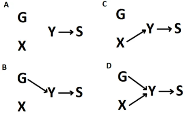
Figure 1.3: Directed acyclic graphs representing the different relationship between a SNP G, a secondary phe-notypeX, a primary phenotypeY and the sampling processS. Here we assume that the sampling process depends only on the primary phenotype. A: There is no association betweenG,X, andY, B:GinfluencesY, C:XinfluencesY, D:Y influencesX, E:GandXinfluencesY, F:GinfluencesY andY influencesX. Bias will occur when estimating the effect ofGonXin scenarios B to F. Scenarios D and F induce reverse causality problems and are not considered in this thesis.
In general, the primary and secondary phenotypes are expected to be correlated as they are collected on the same individual. In this case and for the multiple cases studies we consider in this thesis, the sampling distribution of the secondary phenotypes in the study sample is not representative of its distribution in the general population. A naive analysis which ignores this feature will lead to biased estimates of the effect of genetic variants on the secondary phenotype.
In case-control studies, inverse-probability-weighting approaches (Richardson et al., 2007; Monsees et al., 2009) have been proposed to deal with the sampling mechanism on the primary phenotype. Inverse-probability-weighting is an alternative to regression-based adjustment of the outcomes. This approach focus on the idea that individuals have unequal probabilities to be sampled. To correct for bias induced by the sampling mech-anisms and obtain proper estimates in the population of interest individuals are weighted by their inverse probability to be included in the study. Therefore, giving a larger weight to individuals having a small probability to be included in the study. This approach is very efficient and simple but can create imbalance if weights are not properly com-puted. Therefore, proper modelling of the probability of being included in the study is needed. For family studies, the use of inverse-probability-weighting methods is challeng-ing (Rodríguez-Girondo et al., 2018) because we need to compute the probability that a family is recruited in the study which is not available for our studies. Alternatively, the retrospective likelihood approach can be used. The retrospective likelihood, as explained in Section corrects 1.3.2, implicitly for the ascertainment as follows:
P(X,G|Y,S) =P(S|Y,G,X)P(G,X|Y)
Thus under the assumption that the ascertainment depends only on the case-control status, we require modelling: P(X,G | Y)which using the Bayes rule is further re-written as:
P(X,G|Y) =P(X,Y|G)P(G)
P(Y)
To study the effect of a genetic variant on secondary phenotype we need to explicitly model the correlation betweenXandY. In the case whereX andY are both continuous then we can assume multivariate normal.
In our case, we have a mix of outcomes and thus we build the joint distributions using latent variables. This model is presented in detail in Chapter 2.
1.5
Correlated predictors
An important complication in the discovery of biomarkers associated with a pheno-type and in the prediction of disease phenopheno-types is the complex correlation structure of features and the fact that most phenotypes are associated with a combination of biomark-ers from various omic sources. As a matter of fact, only few diseases are single gene disorders and most of the disease are due to a complex combination of biological and environmental factors.
In this case, separate analysis of omic features using univariate regression models is not advisable. The non-independence of the separate statistical tests and the strong mul-tiple testing correction penalty, due to the high number of omic features, limit the ability of univariate models to discover new associations. A simple solution is then to include all variables of interest as covariates in a multiple regression model. LetY be the quantita-tive phenotype of interest andX= (X1;. . .;XK) a set of biomarkers. The linear model
is written as:
Y=α+
K X k=1
βkXk+
withαthe intercept of the model,βkthe effect size of thekthbiomarker, andthe vector
1.5 Correlated predictors 11
hard to interpret. Finally, the presence of strong correlations increases the possibility of confounder effects and therefore the quantity of false positive associations.
A solution to overcome these issues is to incorporate the correlation structure in the model. In particular, a two-step procedure may be followed. In the first step, the goal is to identify groups of closely related variables. In the second step, this grouping informa-tion is used in the statistical analysis. For the first step, there are two possibilities: either use a Biology- or a data-driven approach. In the biology-driven approach the idea is to incorporate the knowledge about pathways, i.e. groups of single omic features working on a specific cellular function. However, this approach has some limitations: first, the relationship between the variables from the same pathways are not always linear and thus these variables might not be correlated, and second, our knowledge about pathways is still incomplete and therefore we incorporate only a partial picture of the data structure in the model. For the data-driven approach the idea is to empirically derive the correlation structure of the data and to apply clustering algorithms in order to identify clusters of strongly correlated variables. Network construction methods are discussed in Chapters 5 and 6.
Once the groups of omic features have been identified, we can proceed with the statis-tical analysis of step 2. As far as testing is concerned, one approach is to use the grouping information for dimension reduction and then test for association between omics and phe-notypes. In particular, this can be done either by selecting the most "important" variable of the cluster based on a specific criterion or by using a summary measures such as the mean or the first principal component (Pearson, 1901). Association between phenotypes and the summary measures can then be tested in order to detect the group of variables related to these phenotypes. Advantages of such an approach are that it is straightforward to sum-marize clusters of features in one variable and that we considerably reduce the number of tests to be performed. A downside of this approach is that the use of summary measures makes it hard to reproduce the original results. In prediction models, the grouping in-formation can be incorporated in the statistical analysis, via group penalization methods (Yuan and Lin, 2006; Jacob et al., 2009; Simon et al., 2013; van de Wiel et al., 2014). Thereby, only the most important groups needed for the prediction will be selected lead-ing to more stable and easier to interpret prediction models. Note that recently methods have been developed which allow features to be in different clusters allowing the data to mimic more closely the reality as many biomarkers are part of several pathways. These methods are presented and discussed further in detail in Chapters 5 and 6.
1.6
Outline of the thesis
The rest of this thesis contains 5 chapters. As explained in the previous sections, the analysis of omics data can be complicated by several sources of correlation. Table 1.1 shows the correlation structures handled in the different chapters. All chapters may be read in any preferred order, as they have been published or submitted independently. However, we feel that the order in which this thesis has been organized enhances the understanding of the links between the topics of the different chapters. In particular, even though Chapters 2 and 3 both focus on the ascertainment correction for secondary phenotypes in family study designs, we feel that Chapter 3 should be read after 2 as the methodology applied in Chapter 3 is developed in Chapter 2. Chapter 4 may be regarded as the link between the first part (Chapters 2 and 3) and the second part of the thesis (Chapters 5 and 6). In Chapter 4, we still consider family study designs but we use an alternative approach to test for associations between omics data and disease phenotypes, namely correlation networks. Correlation networks are the key ingredient in Chapters 5 and 6, where novel network-based approaches are presented to perform prediction of outcomes in population-based studies with one and multiple omic sources, respectively.
Dependencies Individuals Outcomes Features
Chapter 2 X X
Chapter 3 X X
Chapter 4 X X
Chapter 5 X
Chapter 6 X
Table 1.1: Overview of the between units dependencies modelled in the different chapters of this thesis.
In Chapter 2, we present a novel approach for the analysis of secondary phenotypes in multiple-cases family studies, i.e. families selected for having at least a certain number of cases. In particular, we work under the retrospective likelihood approach and explic-itly model the dependence of the secondary phenotypes and the case-control status using a latent variable approach. A shared random effect is assumed to model the association between the primary and secondary outcome. For the analysis of the primary and sec-ondary phenotypes properly chosen mixed-effects models are used to address the familial relationships. The performance of this approach is empirically evaluated in terms of bias, type I error and robustness to model misspecification. We use the LLS to illustrate the methods.
1.6 Outline of the thesis 13
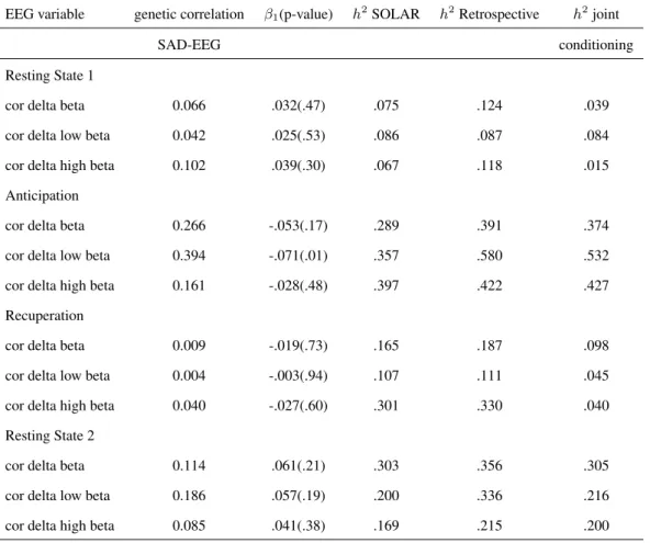
phenotypes in this case, the conditioning on proband approach is typically considered. This approach has been recently applied for the analysis of secondary phenotypes (Green-wood et al., 2007; Turetsky et al., 2015) collected under the proband design. However, the dependency between the primary and secondary phenotypes is not modelled. Therefore, in the context of proband designs we compared our method presented in Chapter 2 with the conditioning on proband approach. Both methods are compared in terms of bias in the estimates of genetic effect on secondary phenotypes and heritability in an extensive simulation study. The relative performance of the two methods has been illustrated on electroencephalography (EEG) data from the LFLSAD.
Chapter 4 presents weighted gene coexpression analysis (WGCNA) with family data using a meta-analysis approach. To take into account between family variation, we pro-posed to perform the WGCNA on each family separately and to combine the obtained results using a meta-analysis approach. This approach was compared with two ad-hoc ap-plications of WGCNA: (1) ignoring the family structure and (2) decorrelation of the gene expression via use of mixed models. To compare their performance, each method was ap-plied on the simulated dataset provided by the Genetic Analysis Workshop 19 (GAW19). Chapters 5 and 6 present network-based approaches for the prediction of health out-comes using omic sources. In particular, Chapter 5 investigates the combination of net-work analysis to identify clusters of correlated variables and the incorporation of this information in group penalization in order to improve stability and prediction ability of prediction model using a single omic source. We have considered several combinations of network analysis methods and group regularization approaches. Specifically, as network construction approaches we have used WGCNA and gaussian graphical modelling and as group regularization approaches we have considered: the group lasso, sparse group lasso, and adaptive group ridge. These combinations are compared with common regularization approaches such as lasso, ridge, and elastic net in terms of prediction ability and vari-able selection via double cross-validation. All methods have been applied to two different datasets: (1) the Dietary, Lifestyle, and Genetic determinants of Obesity and Metabolic syndrome (DILGOM) study where gene expression and metabolomics at baseline were used to predict BMI after 7 years follow-up, and (2) the publicly available breast cancer cell line pharmacogenomics dataset in which we predict the response to treatment of cell lines using gene expression.
ad-ditional step consisting of building a new network of summary measures of the clusters obtained in the first step. Clusters containing related summary measures from differ-ent omic sources are obtained, and clusters containing features from both omics sources can then be derived from them. Finally, the group penalization is performed using an overlapping group lasso approach allowing the variables to be in different groups. The performance of these approaches has been assessed using metabolomics and gene expres-sion data from the DILGOM study and CNV and gene expresexpres-sion from the breast cancer cell line pharmacogenomics dataset to predict the same outcomes as in Chapter 5.
R codes of the methods developed in Chapters 2-3, Chapters 4-5, and supplementary materials of the different chapters can be found at the git repository:
2
Secondary Phenotype Analysis in
Ascertained Family Designs: Application
to the Leiden Longevity Study
Abstract
The case-control design is often used to test associations between the case-control status and genetic variants. In addition to this primary phenotype a number of additional traits, known as secondary phenotypes, are routinely recorded and typically associations between genetic factors and these secondary traits are studied too. Analysing secondary phenotypes in case-control studies may lead to biased genetic effect estimates, especially when the marker tested is associated with the primary phenotype and when the primary and secondary phenotypes tested are correlated. Several methods have been proposed in the literature to overcome the problem but they are limited to case-control studies and not directly applicable to more complex designs, such as the multiple-cases family studies. A proper secondary phenotype analysis, in this case, is complicated by the within fami-lies correlations on top of the biased sampling design. We propose a novel approach to
This chapter has been published as: Renaud Tissier, Roula Tsonaka, Simon P. Mooijart, P. Eline Slag-boom, Jeanine J. Houwing-Duistermaat (2017). Secondary Phenotype Analysis in Ascertained Family Designs: Application to the Leiden Longevity Study.Statistics in Medicine36(14), 2288-2301.
accommodate the ascertainment process while explicitly modelling the familial relation-ships. Our approach pairs existing methods for mixed-effects models with the retrospec-tive likelihood framework and uses a multivariate probit model to capture the association between the mixed type primary and secondary phenotypes. To examine the efficiency and bias of the estimates we performed simulations under several scenarios for the asso-ciation between the primary phenotype, secondary phenotype, and genetic markers. We will illustrate the method by analysing the association between triglyceride levels and glucose (secondary phenotypes) and genetic markers from the Leiden Longevity study, a multiple-cases family study that investigates longevity.
2.1
Introduction
2.1 Introduction 17
modelling secondary phenotypes in these studies.
In the context of case-control studies Monsees et al. (2009) showed that bias can occur when estimating the SNP effect on secondary phenotypes if the primary and secondary phenotypes are associated. This is often the case because both outcomes are measured on the same subjects and secondary phenotypes are typically chosen for their potential associations with the primary phenotype. They also showed that the amount of bias is dependent on the prevalence of the primary phenotype, the strength of the association between the primary and secondary phenotypes, and the association between the tested marker and the primary trait (see Figure 2.1).
Figure 2.1: Directed acyclic graph representing the case where bias is expected when estimating the association between the genetic marker and the secondary phenotype. Arrows represent existing association between each node of the graph. A secondary phenotype analysis investigates whether there is an association between the genetic factor and the secondary phenotype
To deal with the bias problem, investigators first used ad hoc methods i.e. using con-trols only, cases only, combined data of cases and concon-trols or joint analysis of cases and controls adjusting for the case-control status. However, several authors showed that these simple approaches can lead to false positive results (Monsees et al., 2009; Lee et al., 1997; Lin and Zeng, 2009). This is due to the sampling design, namely, the secondary phenotype data are not sampled according to the case-control design as the primary phenotype. Sev-eral sophisticated methodologies have been developed to correct for the sampling mecha-nisms and provide unbiased genetic effect estimates: (i) inverse-probability-of-sampling-weighting approaches (Monsees et al., 2009; Richardson et al., 2007; Schifano et al., 2013) which correct for the sampling mechanism by weighting appropriately individuals in case-control studies, (ii) retrospective likelihood-based approaches which indirectly ad-just for ascertainment (Lin and Zeng, 2009; He et al., 2011), and (iii) a weighted combina-tion of two estimates obtained with the retrospective likelihood approach in the presence or not of an interaction between SNPs and primary phenotypes (Li and H., 2012).
cannot be ignored and therefore it is evident that statistical methodology for proper sec-ondary phenotypes analysis in this context is needed. To this end, under the retrospective likelihood framework, we develop a multivariate probit regression model inspired by the work of Najita et al. (2009) to model jointly the distribution of the primary and secondary phenotype. This approach allows us to deal with the ascertainment issue while taking into account the individual relatedness and the genetic and environmental variations.
The paper is organised as follows: in Section 2, we present the retrospective likeli-hood approach to correct for the over sampling of long-lived subjects and the multivariate probit regression model for the joint modelling of the mixed type primary and secondary phenotypes. In Section 3, we evaluate empirically the performance of the method in terms of bias and efficiency and contrast it with the naive approach which ignores the sampling mechanism. Finally, in Section 4 we illustrate the potential of our proposed method in the analysis of triglyceride levels and glucose in the LLS.
2.2
Methods
2.2.1
Retrospective likelihood approach
LetN be the total number of families in the study. For the familyi(i= 1. . . N) of sizeni, letYi,XiandGibe theni×1vectors for the case-control status, the secondary
phenotype and the genotype, respectively. Motivated by the LLS, we will work under the retrospective likelihood approach to correct for the ascertainment of the families. Such an approach is attractive when modelling the ascertainment mechanism is not straightfor-ward, as in the LLS where sampling depends on the previous generation (an example of a pedigree in LLS is shown in Figure 2.2). In fact the retrospective likelihood approach implicitly corrects for the ascertainment mechanism, under the assumption that the ascer-tainment depends only on the primary phenotypeY. In particular, for theith family it holds:
P(Xi, Gi|Yi, Asc) =
P(Asc|Yi, Gi, Xi)P(Gi, Xi|Yi)
P(Asc|Yi)
=P(Xi, Gi|Yi), (2.1)
withAscthe ascertainment process. By applying Bayes rule we obtain:
P(Xi, Gi|Yi) =
P(Xi, Yi |Gi)P(Gi)
P(Yi)
= PP(Xi, Yi|Gi)P(Gi)
g∈GP(Yi|g)P(g)
. (2.2)
To fully specify (2.2) we need to model properly: the conditional joint distribution of the primary and the secondary phenotypes given the genotype P(Xi, Yi | Gi), the
marginal probability of the primary phenotype P(Yi | Gi), and the genotype probability
of theith family P(Gi). Each one of these elements are described in Sections 2.2.2 and
2.2 Methods 19
Figure 2.2: Example of a family pedigree from the LLS. Squares and circles represent men and women respec-tively, crossed symbols represent deceased individuals. In black are the long-lived individuals on whom the ascertainment is based, in grey are the cases of the study (offsprings of long-lived siblings) and in white are the controls.
2.2.2
Mixed-effects models for the analysis of family data
To model the correlation of the phenotypes Y and X within families, a common choice is to use random effects. For the binary primary phenotype we propose to use a multivariate probit model with random effects. The advantage of this model is that it involves only the integrals of the multivariate normal cumulative distribution function for which efficient algorithms have been developed. In contrast, for the more commonly used logistic regression model, the integrals have to be approximated for example by using Gauss-Hermite quadrature which might be computationally intensive for large pedigrees. LetbY
i = bYi1, . . . , bYini
T
be a set of family specific random effects designed to handle
familial genetic correlation andGi= (gi1, . . . , gini)
T
be the vector of genotypes for fam-ilyi. For the probit model, the observed responseY is viewed as a censored observation from an underlying continuous latent variableY∗with:
Yij =yij ⇔γyij < Y
∗
ij< γyij+1, Yij∈ {0,1}, j= 1,2, ..., ni
where−∞=γ0< γ1 < γ2= +∞are suitable threshold parameters. For the
under-lying latent variableY∗we assume the mixed-effects regression model
Yi∗=α0+α1Gi+σGYb
Y i +σ
Y i ,
whereY
i ∼Nni(0, Ini)is independent ofb
Y
i . Hereα = (α0, α1)denotes the
re-gression coefficient vector withα0 the intercept andα1the parameter representing the
effect of the genotype onY. At the family level we assumebY
i ∼Nni(0,Ri), withRi
the coefficient of relationships matrix with elementsrlm= 2−dlmwithdlmdenoting the
genetic distance between subjectslandmin the family. The parameterσGY represents
polygenic inheritance in a family.
For identifiability reasons restrictions are required on both the scale and location of Y∗, namely we setσ2 = 1 andγ
1 = 0. Thus, in the mixed-effects probit regression
the disease riskπij = P(Yij = 1 | bYij, gij)conditional on the random-effectsbYij and
genotypic informationgijis modelled as follows
P Yij= 1|gij, bYij
= Φ α0+α1gij+σGYb
Y ij
, (2.3)
withΦ (z)the cumulative distribution function of the standard normal distribution. The marginal density under the probit model takes the form:
f(yij|gij;α, σb) = Z
bY i
Z γyij+1
γyij
f(y∗ij|gij, bYi ;α, σb)f(bYi )dy
∗
ijdb Y i .
To model the secondary phenotypeXiwe use a linear mixed model:
Xi =β0+β1Gi+σGXb
X
i +σXi , (2.4)
whereβ= (β0, β1)denotes the regression coefficient vector withβ0the intercept and
β1the parameter representing the effect of the genotype onX,bXi ∼Nni(0,Ri)is the
random parameter used to model the genetic correlation structure within each family for the secondary trait, andσis the residual standard deviation.
To model jointlyXandY using the model specifications (2.3 and 2.4), we introduce a shared random effectuij ∼N(0,1)and propose the following model:
Yi∗=α0+α1Gi+σGYb
Y
i +σuui+Yi ,
Xi=β0+β1Gi+σGXb
X
i +δσuui+σXi ,
(2.5)
whereuiis assumed to be independent ofbYi , biX, Yi , andXi . We introduce a
coef-ficientδin order to have different phenotypic variances for the random effectui. In case
of small datasets or small family sizes, it can be better to constrainδto be equal to 1 for a simpler model. LetΣXiandΣYi∗denote the corresponding variance-covariance
matri-ces of the marginal distributions ofXiandYi∗and letΣXY∗
i be their covariance. The joint
distribution ofY∗andXis then(Yi∗, Xi)vN2ni
α0+α1Gi
β0+β1Gi
,
Σ Y∗
i ΣXYi∗
ΣXY∗
i ΣXi
.
In the special case forni= 2, the variance-covariance matrix becomes:
Σi=
σ2
GY +σ
2
u+ 1 σ2GY2
−d(1,2) σ
GXσGY +δσ
2
u σGXσGY2
−d(1,2)
σG2
Y2
−d(1,2) σ
GY +σ
2
u+ 1 σGXσGY2
−d(1,2) σ
GXσGY +δσ
2
u
σGXσGY +δσ
2
u σGXσGY2
−d(1,2) σ2
GX +δ
2σ2
u+σ2 σG2X2
−d(1,2)
σGXσGY2
−d(1,2) σ
GXσGY +δσ
2
u σ2GX2
−d(1,2) σ2
GX +δ
2σ2
2.2 Methods 21
Using the properties of the multivariate normal distribution, the joint distribution for the observed primary and secondary phenotypes takes the form:
P(Yi, Xi|Gi) = Z
P(Yi∗, Xi|Gi)dyi∗
=
Z
P(Yi∗|Xi, Gi)P(Xi|Gi)dyi∗
=P(Xi|Gi) Z
P(Yi∗|Xi, Gi)dyi∗.
Thus by using the probit regression model for the primary trait we have developed an efficient approach to model the correlation between the primary and secondary trait.
From model (2.5) and the variance-covariance matrix (2.6), several marginal correla-tions between and within family members can be deduced:
cor(Xij, Xij0) =
σ2
GX2
−d(j,j0)
σ2
GX +δ
2σ2
u+σ2 =ρX
cor Yij∗, Yij∗0
= 2
−d(j,j0)
σ2
GY
σ2
GY +σ
2
u+ 1 =ρY
cor Xij, Yij∗
= σGXσGY +δσ
2
u q
σ2
GX +δ
2σ2
u+σ2
σ2
GY +σ
2
u+ 1
=ρXY
cor Xij, Yij∗0=
2−d(j,j0)σGXσGY
q
σ2
GX +δ
2σ2
u+σ2
σ2
GY +σ
2
u+ 1
=ρ0XY,
whereρXY represents the association between the primary and secondary phenotype.
We can also derive the closed form for the heritability estimates of the secondary pheno-type which quantifies the percentage of genetic variation in the total variance:
H2= σ
2
GX
σ2
GX+δσ
2
u+σ2
. (2.7)
Note that when genetic factors are included in the model formula (3.2) gives the resid-ual heritability.
2.2.3
Genotype probability
Finally another key component in the formulation of the retrospective likelihood (2.2) is the computation of the genotype probability for each familyi. LetGmjandGpjdenote
P(Gi) = J Y j=1
(
P(gij|Gmj, Gpj) ifjis a nonfounder
P(gij) ifjis a founder
.
The probabilities P(gij | Gpj, Gmj)are the transmission probabilities which can
be modelled using mendelian inheritance. Finally P(Gpi), P(Gmi), and P(gij) can
be modelled by assuming Hardy-Weinberg proportions(1−q)2, 2q(1−q),q2 which
depend onq, the minor allele frequency. Here we propose to use external information forq or to estimateqfrom the control sample before maximizing the likelihood. Note that when genotypes of the parents are missing the probability can be obtained by summing over the possible parental genotypes. In case of more complex pedigree a recursive algorithm known as peeling (Elston and Stewart, 2013) can be used . For the LLS where families are sibships the probability is as follows:
L(θ;Y, X) =Y
i
{P(Xi|Gi)RP(Yi∗|Xi, Gi)dy∗i}
P
Gp
P
Gm
Q
jP(Gij|Gm, Gp)P(Gp)P(Gm)
P g P Gp P Gm R P Y∗
i |g
P(g|Gm, Gp)P(Gp)P(Gm)
,
(2.8)
whereθ= (α0, α1, σGY, β0, β1, σGX, σ, δ, σu)is the model parameters vector.
2.2.4
Estimation and statistical testing
To estimate the parameters of the joint model we maximize the logarithm of the like-lihood described in (2.8). This involves a combination of numerical optimization and integration. For the evaluation of the integral in the multivariate normal distribution, we use the deterministic algorithm Miwa described in Miwa et al. (2003). For the optimiza-tion, we use the Broyden-Fletcher-Goldfarb-Shanno (BFGS) algorithm implemented in the functionoptim(.) in R. The BFGS algorithm is a quasi-Newton method, which means that the Hessian matrix does not need to be evaluated directly but is approximated by using specified gradient evaluations. To test for the presence of an effect of the SNPs on the secondary phenotype we use the likelihood ratio test. Note that when the interest of a researcher is solely testing for genetic association a score statistic is an alternative to the likelihood ratio statistic.
2.2.5
Continuous polygenic score
Our approach can also be applied in the case of modelling the association between continuous covariates and secondary phenotypes. For example polygenic scores have been used to summarise genetic effects among an ensemble of SNPs that have been iden-tified in large GWASes (International Schizophrenia Consortium et al., 2009; (IMSGC) et al., 2010; Simonson et al., 2011). Polygenic scores are typically linear combinations of SNPs: G=P
kδkSN Pk, whereδk = 1orδk is obtained from previous GWASes. For
2.3 Simulation Study 23
the mean value of the genetic score,σgthe standard deviation of the genetic score andRi
the relationship matrix of familyi. The likelihood contribution for familyiis given by:
P(Yi, Xi|Gi)P(Gi)
P(Yi)
= P(YRi, Xi |Gi)P(Gi) y∗
i
P(y∗i)dyi∗ =
P(Yi, Xi|Gi)P(Gi) R
y∗
R giP(y
∗
i |gi)P(g)dyi∗dgi
.
Computation of the integral R y∗
R gP(y
∗ | g)P(g)dy
∗dgcan be quite intensive and
challenging. In order to gain efficiency we write the marginal model ofY∗(2.5) asYi∗=
α0+bYi ∗ +ui+Yi , with b Y∗
i = σGYb
Y
i +α1Gi. Now Yi∗ follows the following
multivariate normal distribution: Yi∗ v Nni α0+α1µg,ΣYi∗+α
2 1σ
2
gRi
. Note that when a polygenic risk score is included in the model for the secondary phenotype, the parameterσGY represents the residual polygenic inheritance.
2.2.6
Inclusion of covariates in the model
Often, researchers want to adjust for covariates such as age, sex, treatment etc in the model. LetZbe such a covariate. To estimate the effectZ on the secondary phenotype we propose to maximize the joint likelihood ofX andGconditionally on the primary phenotype Y andZ. Thereby we avoid modeling of the distribution of Z within the families. Indeed, under the assumption of independence between genotype andZ we obtain:
P(Xi, Gi|Yi, Zi) =
P(Xi, Yi, Zi, Gi)
P(Yi, Zi)
=P(Xi, Yi|Gi, Zi)P(Gi)P(Zi)
P(Yi|Zi)P(Zi)
(2.9)
=P(Xi, Yi|Gi, Zi)P(Gi)
P(Yi|Zi)
.
2.3
Simulation Study
With respect to the familial relationships, we consider only sibships such that our simula-tion resembles the LLS design. For the prevalence of the primary phenotype we consider two settings namely a disease prevalence of 1% which corresponds toα0 ≈ −2.32and
of 5% which corresponds toα0≈ −1.64. In addition the variance parameters have been
chosen such that they correspond to a heritability of 50%. Specifically we useσGX=2,
σGY =
√
3,σuX = σuY =
√
2 andσ =
√
2. This corresponds to a correlation of 0.78 between the primary and the secondary phenotypes. To speed up computations, we assume thatσuX = σuY when fitting the models to the simulated datasets. For each
scenario, 500 datasets are simulated using model (2.5).
2.3.1
Simulation results for a SNP
The genotypes of the SNPs are simulated assuming a minor allele frequency of 0.3 in the population. For the secondary phenotype model the following fixed effects values are used:β0 = 3.5andβ1= 0.2, whereas for the primary phenotype model the effect sizes
areα1=0.1 or 0.5. Finally, for each of the four scenarios (rare or common disease, and
weak and strong SNP effect on the primary phenotype) we consider two ascertainment mechanisms, namely the sampled sibships of size five have at least one affected or at least two affected members.
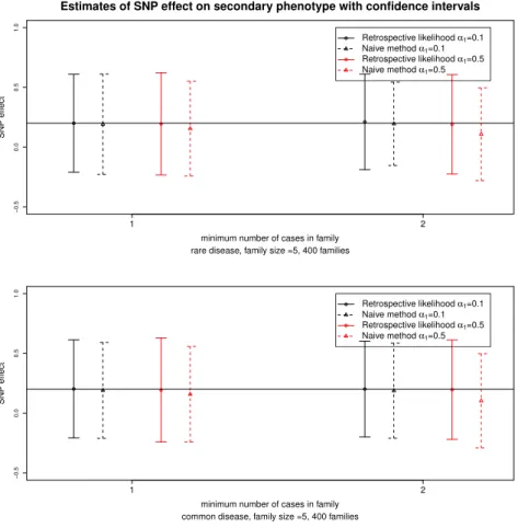
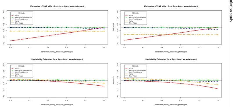
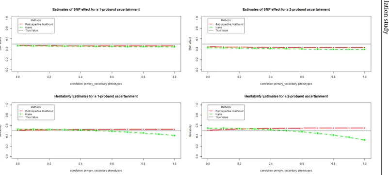
Figure 3.3 presents the estimates and 95% confidence intervals for the scenario of 400 sibships. Figure 3.3 shows that ignoring the sampling mechanism (naive method) leads to biased estimates of the SNP effect and the size of this bias increases with the strength of the ascertainment mechanism and the association between the SNP and the primary phenotype. Overall we observe that the proposed method gives unbiased estimates of the SNP effect on the secondary phenotype. The coverage probabilities reach the nominal level (see section A of supplementary material). Regarding the prevalence of the primary phenotype, we observe that for the naive method bias increases with lower prevalence, while the proposed method remains robust to the lower amount of information due to the rare primary phenotype. In general, the proposed method leads to smaller RMSE than the naive approach and better coverage probabilities.
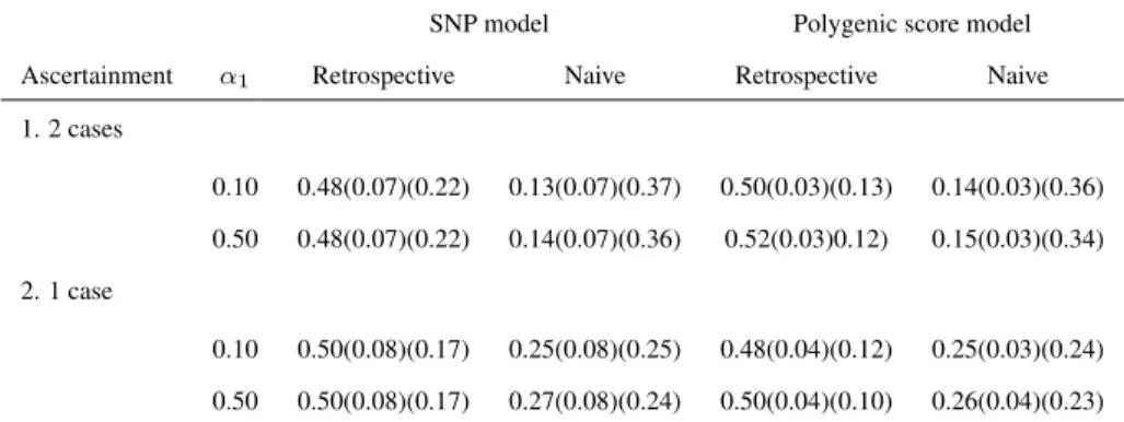
In Table 2.1 we present the heritability estimates of the secondary phenotype for a common disease, under the various ascertainment mechanisms and the two values ofα1.
It is obvious that the heritability estimates are influenced by the ascertainment mecha-nisms when using the naive approach. Indeed the naive method tends to underestimate the heritability for each mechanism and this underestimation increases as the ascertainment mechanisms become more stringent. The heritability estimates are 25-27% for sibships with at least one affected sibling and drop to 13-14% for sibships with at least 2 affected siblings. On the contrary, the proposed method is robust to the stringency of the ascer-tainment mechanism.
2.3 Simulation Study 25
−0.5
0.0
0.5
1.0
Estimates of SNP effect on secondary phenotype with confidence intervals
minimum number of cases in family
SNP eff
ect
1 2
rare disease, family size =5, 400 families
Retrospective likelihood α1=0.1
Naive method α1=0.1
Retrospective likelihoodα1=0.5
Naive method α1=0.5
−0.5
0.0
0.5
1.0
minimum number of cases in family
SNP eff
ect
1 2
common disease, family size =5, 400 families
Retrospective likelihood α1=0.1
Naive method α1=0.1
Retrospective likelihoodα1=0.5
Naive method α1=0.5
Figure 2.3: Estimates and 95% confidence intervals for the SNP effect on the secondary phenotype for the retrospective likelihood approach and the naive method. Results are obtained from 500 simulated datasets of 400 families for 2 ascertainment schedules. The top and bottom panel correspond to a rare or common primary phenotype with a prevalence around 1% and 5% respectively. In black and red are represented results for small (α1=0.1) and large (α1=0.5) effect sizes of the SNP on the primary phenotype, respectively. The horizontal line
corresponds to the true SNP effect on the secondary phenotype.
in Table 2.2. These results show that even though our approach gives biased estimates for the primary phenotype model, the parameters estimates for the secondary phenotype model are not affected. All the results are presented in Section A of the Supplementary Material.
SNP model Polygenic score model
Ascertainment α1 Retrospective Naive Retrospective Naive
1. 2 cases
0.10 0.48(0.07)(0.22) 0.13(0.07)(0.37) 0.50(0.03)(0.13) 0.14(0.03)(0.36)
0.50 0.48(0.07)(0.22) 0.14(0.07)(0.36) 0.52(0.03)0.12) 0.15(0.03)(0.34)
2. 1 case
0.10 0.50(0.08)(0.17) 0.25(0.08)(0.25) 0.48(0.04)(0.12) 0.25(0.03)(0.24)
0.50 0.50(0.08)(0.17) 0.27(0.08)(0.24) 0.50(0.04)(0.10) 0.26(0.04)(0.23)
Table 2.1: Heritability results of the simulation studies for a SNP and a polygenic score: Estimates with stan-dard deviations and RMSE (in brackets) for the heritability of the secondary phenotype for a common disease (prevalence≈5%), when families with at least one and at least two cases are sampled and for two values ofα1,
i.e. SNP or polygenic score effect on primary phenotype. Datasets consist of 400 families of size 5. Results are based on 500 replicates.
Ascertainment α1 β1 heritability
0.True value 0.200 0.500
1.At least 2 cases
0.100 0.199(0.104)(0.104)(0.948) 0.509(0.017)(0.110)
0.500 0.197(0.106)(0.110)(0.945) 0.516(0.014)(0.108)
2.At least 1 case
0.100 0.200(0.104)(0.107)(0.961) 0.510(0.012)(0.096)
0.500 0.199(0.107)(0.111)(0.960) 0.513(0.010)(0.087)
Table 2.2: Robustness: Estimates of the effect size of the SNP on the secondary phenotype (β1) and heritability
of the secondary phenotype are given for a common disease (prevalence≈5%), for the two ascertainment mechanisms and two values ofα1. Into brackets are standard deviations, RMSE and coverage probability (for
2.3 Simulation Study 27
nominal level (α) Retrospective likelihood Naive method
At least 2 cases
α1=0.1
0.05 0.0509 0.0580
0.01 0.0118 0.0152
0.001 0.0017 0.0025
α1=0.5
0.05 0.0505 0.0878
0.01 0.0113 0.0222
0.001 0.0013 0.0043
At least 1 case
α1=0.1
0.05 0.0524 0.0514
0.01 0.0102 0.0098
0.001 0.0018 0.0014
α1=0.5
0.05 0.0522 0.0558
0.01 0.0098 0.0097
0.001 0.0009 0.0016
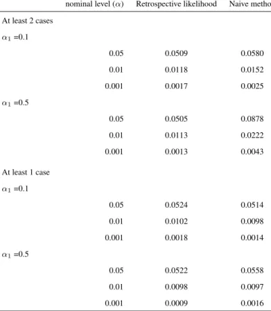
Table 2.3: Type I errors rates for testing for association between a genetic marker and a secondary phenotype for four scenarios. Families with at least one and with at least two cases are considered. Two values for the association between the SNP and the primary phenotype namelyα1= 0.1 andα1= 0.5 are used. Datasets
consist of 400 families of size 5. Results are based on 10000 replicates.
each of the four considered scenarios, we simulate 10,000 replicates. In Table 3.2 the emprical type I error rates are given for the rare disease scenario (i.e. prevalence 1%). We observe that while our approach preserves the type I error rate at a nominal level, the naive approach has, systematically, an inflated type I error rate. The type I error rate for the naive method increases with stronger ascertainment and larger SNP effect on the primary phenotype.
2.3.2
Simulation results for a polygenic score
chosen as for the SNP simulations:β0= 3.5andβ1= 0.2, whereas for the primary
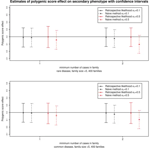
phe-notype model effect sizes ofα1=0.1 or 0.5 were used. Figure 3.4 presents the estimates
and confidence intervals for datasets with 400 sibships. Our approach provides unbiased estimates of the effect of the polygenic score on the secondary phenotype. In contrast, the naive approach provides biased estimates and the bias increases when the ascertainment process is more stringent or whenα1is larger.
−0.1
0.0
0.1
0.2
0.3
0.4
0.5
0.6
Estimates of polygenic score effect on secondary phenotype with confidence intervals
minimum number of cases in family
Polygenic score eff
ect
1 2
rare disease, family size =5, 400 families
Retrospective likelihood α1=0.1
Naive method α1=0.1
Retrospective likelihoodα1=0.5
Naive method α1=0.5
−0.1
0.0
0.1
0.2
0.3
0.4
0.5
0.6
minimum number of cases in family
Polygenic score eff
ect
1 2
common disease, family size =5, 400 families
Retrospective likelihood α1=0.1
Naive method α1=0.1
Retrospective likelihoodα1=0.5
Naive method α1=0.5
Figure 2.4: Estimates and 95% confidence intervals for the polygenic score effect on the secondary phenotype for the retrospective likelihood approach and the naive method. Results are obtained from 500 simulated datasets of 400 families for 2 ascertainment schedules. The top and bottom panel correspond to a rare or common primary phenotype with a prevalence around 1% and 5% respectively. In black and red are represented results for small (α1=0.1) and large (α1=0.5) effect sizes of the polygenic score on the primary phenotype, respectively. The
horizontal line corresponds to the true polygenic score effect on the secondary phenotype.
2.4 Application: Analysis of the Leiden Longevity Study 29
approach did not perform well: estimates between 25-26% and 14-15% for an ascertain-ment process of at least one affected sibling and at least two affected siblings respectively instead of 50%.
2.4
Application: Analysis of the Leiden Longevity Study
In this Section, we will exemplify our proposed method in the analysis of the LLS briefly introduced in Section 1. The LLS is a family-based study set up to identify mech-anisms that contribute to healthy ageing and longevity. The inclusion criteria of the study are sibships with at least two nonagenarian siblings, i.e. the selection takes place at Gener-ation II (Figure 2.2). Several secondary phenotypes and GWAS data have been measured for the offspring of these siblings (Generation III in Figure 2.2) and their partners. Since the offspring have at least one nonagenarian parent, they are also likely to become long-lived. Therefore, the set of offspring and their partners corresponds to a case-control design with related subjects where the offspring in Generation III are considered as cases and their partners as controls. Overall 421 families with 1671 offspring (cases) and 744 partners (controls) have been included in the study. Because the families are relatively small we use the model which assumes an equal variance for the shared effect for the two traits.
Here we model the association between genetic factors and the secondary phenotypes triglyceride and glucose levels. For both traits, there is evidence of an association with human longevity and both traits are normally distributed. For the sake of comparison in addition to our proposed method, we will present results using the naive approach i.e. standard linear mixed model. Analyses using the linear mixed model which conditions also on the case-control status will not be presented because the parameters do not have a comparable interpretation between the two approaches. The p-values presented below are obtained using the likelihood ratio test.
2.4.1
Triglyceride levels analysis
Triglyceride levels have been found to be associated with the primary trait longevity (p-value = 0.0005 for women andp-value = 0.04 for men) and the size of association is sex dependent. Therefore a sex-stratified analysis has been considered further. For the purposes of our illustration, we restricted our analysis to seven genes on chromosome 11 which are known to be associated with Triglyceride levels. These genes areAPOA1, APOA4, APOA5, APOC3, ZNF259, BUD13andDSCAML1. The selection of the genes was performed using the NHGRI-EBI GWAS catalog (Welter et al., 2014). For these genes, we have genotypes of 41 SNPs which have no missing values in our datasets. Triglyceride levels were standardized and we included age as a covariate in the analysis.
two approaches. The SNPs showing the largest differences are, in men, SNP 22: βRA
1
= 0.047 for our Retrospective Approach (RA) andβN A
1 = 0.052 for the Naive Approach
(NA) and SNP 26:βRA
1 = 0.088 andβ1N A= 0.092. For women more SNPs give different
estimates between the two approaches, i.e. SNP 1 (βRA
1 = 0.024,β1N A= 0.020), SNP 2
(βRA
1 = 7.2e-06βN A1 =0.006), SNP 13 (β1RA= -0.013,β1N A= -0.009) and SNP 19 (β1RA=
0.011,βN A
1 = 0.007) showed the biggest differences. Results for the SNPs are presented
in Section B of the Supplementary Material.
We verified whether the assumption of equal variances for the primary and secondary phenotype for the shared effects is justified. We fitted also the model with non constrained δ. We noticed that for some of the SNPs the model parameters are hard to estimate and the estimates of the variances of the shared and residual random effects in the model for the second phenotype are swapped. Overall the estimates of the effect of the SNP on the secondary phenotype are very similar to the model which assumes equal variances. Results of these analyses are presented in Section B of the Supplementary Material.
2.4.2
Glucose levels analysis
In previous analysis of glucose levels in the offspring and partners of the LSS, Mooi-jaart et al. (2010) studied the association between glucose and a polygenic score. The ge-netic score was defined as the total number of risk alleles across 15 SNPs which are known to be associated with Type II diabetes. The Generalized Estimating Equation method was applied to take into account the familial relationships. The paper showed that a higher number of Type II diabetes risk alleles is associated with a higher serum concentration of glucose (p−value= 0.016). A statistically significant association was found between glucose level and case-control status (p-value<0.001). However, the sampling process was not taken into account in the analysis and thus the results might be biased. We applied the proposed method to estimate the heritability of glucose levels and to test for the pres-ence of an association between the glucose levels and the polygenic score. In addition, we applied the naive approach which did not correct for case-control status. We did not stratify according to sex in these analyses.
For this analysis the polygenic score was standardized. Using the Retrospective ap-proach, the association between the genetic score and the glucose level is estimated by βRA
1 = 0.630with a standard error ofstE = 0.023(p−value = 0.015). The naive
approach also yields a significant association between the genetic score and glucose lev-els (βN A
1 = 0.622,stE = 0.026,p−value = 0.020). By using the Naive Approach
(NA) we obtained for the glucose levels a genetic variance ofσ2
GX = 0.302and a total
variance ofσ2
T = 1.322, which corresponds to a residual heritability ofh2N A = 0.228.
Our Retrospective approach (RA) yields a genetic variance ofσ2
GX = 0.384and a total
variance ofσ2