Comparative Analysis of Different Path Finding Algorithms to Study Limitations and Progress

(1)

International Journal of Emerging Technology and Advanced Engineering

Website: www.ijetae.com (ISSN 2250-2459, ISO 9001:2008 Certified Journal, Volume 7, Issue 9, September 2017)

68

Comparative Analysis of Different Path Finding Algorithms to

Study Limitations and Progress

Harita Vamja

1

, Ayesha Shaikh

2

, Sonal Rami

3 1_{Student, Dept. of IT, CHARUSAT}

2,3_{Assistant Professor, Dept. of IT, CHARUSAT}

Abstract—Today number of path finding algorithm is being

used in different areas of computer science. It is difficult to find which algorithm is suitable for our application without making detailed analysis of those algorithms. It is required to understand those algorithms properly with their working, application and limitations to design another algorithm according to requirements in practical use. This paper covers working of different path finding algorithms such as Dijkstra’s algorithm, A* and IDA* with a general example along with their limitations and how they are improvised in other algorithms. It finally concludes with a comparative table under different parameters in general.

Keywords— Shortest path-finding, Dijkstra, A*, IDA*, heuristics

I. INTRODUCTION

There are different shortest path-finding algorithms such as Dijkstra, Bellman-Ford algorithm, Floyd-Warshall algorithm, A*algorithm and D* algorithm which are used in real world to solve problems like finding shortest path between two points in map, inversion of real matrices etc. The problem of finding shortest path is difficult in many fields starting from navigational systems to artificial intelligence. Although many shortest path finding algorithms work properly, still, it is difficult to decide that which algorithm is beneficial over other algorithms. Dijkstra is efficient in finding shortest path even with wastage of resources and time due to blind search. A* finds the optimal solution within less time but runs out of memory if state space is large to compute. IDA* is removes the memory constraint of A* but the revisit of nodes increase at each level.

This paper gives basic overview of Dijkstra, A*algorithm, IDA* algorithm along with pseudo code.

The purpose of this paper is to state the limitations of each algorithm and provide possible ways to overcome the limitations. It is based on the general application and approach of algorithms.

II. APPLICATION AREAS OF PATH FINDING ALGORITHM

Path finding algorithms are mostly used in following real time applications:

 To find shortest path between two points (location) in map i.e. navigation systems.

 In social networking to find shortest distance between two persons.

 In finding shortest path in VLSI and facility layout.

 In telephone network to get maximum bandwidth utilization.

 In game programming to find path between two points.

 Network routing protocols- Open Shortest Path First is one of the example to send data faster utilizing minimum resources.

(2)

International Journal of Emerging Technology and Advanced Engineering

[image:2.612.63.277.141.360.2]

69

III. PATH-FINDING ALGORITHMS

Figure I Common Graph [12]

A. Dijkstra’s Algorithm

Dijkstra’s algorithm is shortest path finding algorithm conceived by computer scientist Edsger W Dijkstra in 1956 and was published 3 years later. Dijkstra uses graph as data structure and follows greedy approach. It works as following:

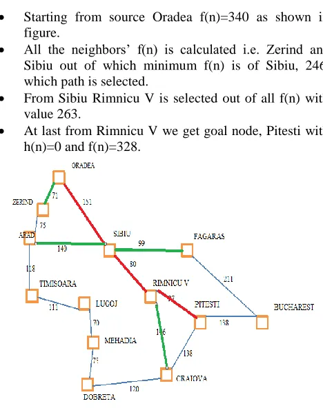
From the common graph let us take Oradea as source and Pitesti as destination.

 Taking distance of source i.e. Oradea as 0 and all other distances as infinity.

 Starting from Oradea considering immediate neighbors Zerind and Sibiu, update the distance from source to each node from infinity to 71 and 151 respectively.

 Consider the lowest value or distance i.e. Zerind and mark that node as visited. From Zerind locate immediate neighbor i.e. is Arad and mark it as visited updating value from 75 to 146.

 From Arad there are two nodes Sibiu and Timisoara update the values 160 and 264. Here the value to Sibiu increases from source then previous which was 151. Hence, the algorithm selects the previous path from source i.e. Oradea to Sibiu with value 151 and mark it as visited. The algorithm checks for shortest path from source to current node via other adjacent nodes so it checks for every possibility.

 From Sibiu it updates the nodes Fagaras and Riminicu to 250 and 231.

 From Riminicu nodes Pitesti and Craiova are updated to 328 and 377.

[image:2.612.328.555.142.462.2]

 Here we find our destination at value 328, Pitesti.

Figure II Dijkstra’s Algorithm

Red line-obtained shortest path Blue line- explored path

1. Pseudo code [1]:

Dijkstra (graph, source): Create vertex set V For each vertex v in graph:

If v ≠ source

dist[v]< infinity prev[v]<undefined add v to V

While V is not empty:

u < vertex in V with min dist[u] remove u from V

for each neighbor v of u: alt <- dist[u]+length(u,v)

(3)

International Journal of Emerging Technology and Advanced Engineering

70

2. Time complexity:

Dijkstra’s time complexity is O(|v|2_{) but it can also be}

implemented as Fibonacci heap as priority queue then complexity can be further reduced to O(|E| +|V|log|V|) where E is edges and V is vertices[5].

3. Applications:

Dijkstra is used in navigational systems in complex form to find shortest distance between two points. It is also used in network routing protocols such as OSPF(open shortest path first). It is used in telephone network to obtain maximum available bandwidth and used as subroutine in Johnson’s algorithm.

4. Improvements:

If we use d-heap(Jhonson,1970) then it reduces the cost to Edlogd(v) and will be easy to implement

[1]

.

5. Limitations:

Dijkstra’s algorithm follows blind search which leads to wastage of resources by consuming a lot of time. As there is no chances of backtracking if we choose an infeasible node then algorithm might go into infinite loop. It cannot handle negative edges leading in acyclic graphs which cannot give optimal result. As in the above example even though shortest distance from source to destination was direct but due to logic of algorithm it took 3 more iteration to reach even first possible shortest node. Hence, to remove the problem of optimality in many cases A* algorithm was devised. The solution to optimal path finding along with reduced time complexity is given in A* algorithm.

B. A* Algorithm

In computer science, A* is an efficient algorithm generally used for path-finding and graph traversal by efficiently plotting directed path between multiple nodes.

Peter Hart, Nils Nilsson and Bertram Raphael of Stanford Research Institute invented the A* algorithm .A* uses dynamic programming to reach goal. A* algorithm has better performance and accuracy than Dijkstra. A* is complete as well as optimal search algorithm. A* algorithm uses graph as data structure and is an informed search algorithm. A* searches for all the immediate neighbors from the current node to find shortest path. A* introduces the most significant characteristic of the algorithm which makes it efficient than others that is heuristics. Heuristic function is used to estimate the cheapest path from current node to goal node and they should be admissible. A* minimizes:

f(n) = g(n) + h(n)

where n is the last node on path, g(n) is cost of the path from start node to n and h(n) is heuristic function. Thus, f(n) is cheapest cost to goal through n. A* uses priority queue managing an opened and closed set. As A* searches in tree manner the explanation is in the same form. Given is the simple explanation of how A* search works with an example.

Estimated straight line distance:

Arad 300

Bucharest 34

Craiova 30

Dobreta 110

Fagaras 65

Mehadia 80

Oradea 340

Pitesti 0

Riminicu V 32

Sibiu 95

Timisoara 229

(4)

International Journal of Emerging Technology and Advanced Engineering

[image:4.612.64.551.122.736.2]

71

Figure III Tree formation of A* search

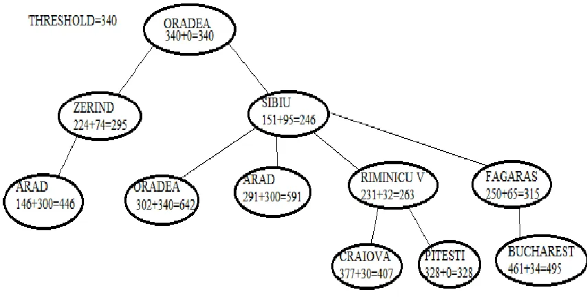
[image:4.612.70.541.137.347.2]

 Starting from source Oradea f(n)=340 as shown in figure.

 All the neighbors’ f(n) is calculated i.e. Zerind and Sibiu out of which minimum f(n) is of Sibiu, 246, which path is selected.

 From Sibiu Rimnicu V is selected out of all f(n) with value 263.

 At last from Rimnicu V we get goal node, Pitesti with h(n)=0 and f(n)=328.

Figure 4 A* Algorithm

Red line-obtained shortest path Green line- explored path

1. Pseudo code [7]:

initialize the open list initialize the closed list

put the starting node on the open list

while the open list is not empty

find the node with the least f on the open list, call it "q"

pop q off the open list

generate q's successors and set their parents to q for each successor

if successor is the goal, stop the search successor.g = q.g + distance between successor and q successor.h = distance from goal to successor successor.f = successor.g + successor.h

if a node with the same position as successor is in the OPEN list \

which has a lower f than successor, skip this successor

if a node with the same position as successor is in the CLOSED list \

which has a lower f than successor, skip this successor

otherwise, add the node to the open list end

[image:4.612.49.283.375.671.2]

(5)

International Journal of Emerging Technology and Advanced Engineering

72

2 .Time complexity:

The time complexity of A* depends on the heuristic, if the function is admissible and better then we get optimal solution with optimal time complexity. In the worst case of an unbounded search space, the number of nodes expanded is exponential in the depth of solution, d= O(bd) where b is branching factor.

3. Applications:

A* is commonly used for path-finding in games. It is also used in solving problem of parsing using stochastic grammars in NLP

4. Improvements:

Bidirectional A* is used an improvement to A* where the main concept is to implement A* search from source as well as destination. In which, it depends on how search at both the end meets.

5. Limitations:

A* search will not give optimal result if heuristics are not admissible. The main limitation of A* is that as it has to save entire open list so it occupies more space in some cases for such as eight queen problem. As it needs more space it still seems quite infeasible to use in practical navigation systems.

6. Improvement over Dijkstra’s algorithm:

As A* uses heuristics, the chances to find optimal solution is far better than Dijkstra. The problem of Dijkstra unable to backtrack is efficiently solved in this by use of heuristics. If admissible heuristics are used than it gives better time complexity than Dijkstra as it does not search all nodes(blind search) but only those with best possibility.

C. IDA* - ITERATIVE DEEPING A* algorithm

IDA* is variant of iterative deepening depth first search but uses heuristics like A* to fasten the search. The algorithm was first developed by Richard Korf in 1985. IDA* uses tree as data structure. This algorithm follows depth first search but does not go to same depth everywhere, so requires less memory and focuses on exploring most promising nodes. Algorithm works in iterations and with each iteration depth first search is performed and if f(n)=g(n)+h(n) exceeds given threshold that branch is cut and search backtracks. Again the whole search starts from beginning. This threshold is initialized to estimate heuristics at starting and increases with each iteration. The algorithm terminates as soon as goal state is reached whose total cost does not exceeds current threshold. IDA* is version of A* which uses memory linear in length of the solution that it finds.

Following is working of IDA* with respect to above example.

 First iteration: Starting with Oradea following depth first search, exploring Zerind and Sibiu with threshold of Oradea with f(n)=340.

 As f(n) for Zerind is 295( and that of Sibiu is 246, we continue to explore the nodes that is Arad with f(n) 446 for Zerind node. Now, for Sibiu Arad with f(n) 591, Rimnicu V with 263 and Fagaras with 315.

 Now we still explore nodes Riminicu V with f(n)=263 going to Craiova with f(n)=407 and Pitesti with f(n)=328, Fagaras going to Bucharest with f(n)=495.

 Here in first iteration goal Pitesti is reached with total cost f(n)=328 which is less then threshold.

Following is the figure with second iteration:

(6)

International Journal of Emerging Technology and Advanced Engineering

[image:6.612.85.512.163.382.2]

73

Figure IV Tree formation of IDA* search

1. Pseudo code[9]:

root=initial node; Goal=final node;

function IDA*() {

threshold=heuristic(Start); while(1)

{

temp=search(Start,0,threshold); search(node,g score,threshold)

if(temp==FOUND) //if goal found return FOUND; if(temp== ∞) //Threshold larger than maximum possible f value

return; //or set Time limit exceeded threshold=temp;}

}

function Search(node, g, threshold) //recursive function

{

f=g+heuristic(node);

if(f>threshold) //greater f encountered return f;

if(node==Goal) //Goal node found return FOUND;

min=MAX_INT; //min= Minimum integer foreach(tempnode in nextnodes(node)) {

//recursive call with next node as current node for depth search

temp=search(tempnode,g+cost(node,tempnode),threshold);

if(temp==FOUND) //if goal found return FOUND;

if(temp<min) //find the minimum of all ‘f’ greater than threshold encountered min=temp;

}

return min; //return the minimum ‘f’ encountered greater than threshold

}

(7)

International Journal of Emerging Technology and Advanced Engineering

74

{

return list of all possible next nodes from node; }

2. Time complexity:

Time complexity of IDA* depends upon different values heuristic function can take. The efficiency of IDA* is as good as A*, as f value increases two or three times in most of cases. Hence, worst time complexity is O(bd), where b is branching factor and d is depth.

3. Applications:

IDA* is used in automated planning and scheduling. It is a branch of artificial intelligence that concerns realization of strategies for execution by intelligent agents and autonomous robots.

4. Improvements:

Simplified memory bound A* search is an improvement to IDA* which utilizes the available space to increase performance efficiency by reducing time complexity to explore repeated nodes. Recursive best first search is another algorithm which is version of A* and is practically faster than IDA* as it regenerates less nodes as compared to IDA*.

5. Limitations:

IDA* algorithm follows depth first search strategy due to which it has to explore nodes repeatedly which is its major limitation. Unlike A* which uses dynamic programming, IDA* has to repeat nodes to reach goal when the threshold is exceeded. It requires more processing power than A* algorithm. IDA* can achieve smaller depth search but not smaller branching factor. In more complex domain like travelling salesman problem IDA* faces difficulty as heuristic value is different for every state.

6. Improvement over A*:

A* search maintained open list which utilized high memory often was outrun by space complexity before time complexity. IDA* is version of A* which uses memory linear in length of the solution that it finds.

IDA* performs search according to depth first search, its space complexity is O(bd) whereas A* space complexity is O(bd) where b is branching factor and d is depth. The major drawback of A* is covered in IDA* which gives equal efficiency in performance.

TABLE1-

COMPARITIVE ANALYSIS OF DIFFERENT PATH FINDING ALGORITHMS ON BASIS OF DIFFERENT PARAMETERS IN

GENERAL:

Parameters Dijkstra’s algorithm

A* algorithm IDA* algorithm

Time complexity

O(v2) where v is vertices or number of nodes

Worst case-O(bd) where b is branching factor and d is depth

Heuristics h(n)

f(n)=g(n)+h (n)

h(n)=0 h(n) = admissible for optimal solution h(n) = admissible for optimal solution Real time application Navigation system, link-state routing protocols, OS PF, telephone networks Navigation system, game programming, parsing, stochastic grammars in NLP Planning, used as replacement of A* in memory constrained areas Limitations with current algorithm Does not always give optimal solution Space complexity outruns before time complexity in large scale for e.g. eight queen problem

Repeated visit to same node as it is not dynamically programmed

(8)

International Journal of Emerging Technology and Advanced Engineering

75

Used in

current GPS navigation as base.

nodes. Can be used in memory constrained situations.

Disadvanta ges

Does not work on negative edge.

No optimal solution guaranteed.

Searches every node(most often) in graph.

Currently not used in GPS navigation systems.

Space complexity outruns time complexity in certain cases.

Nodes are revisited after every iteration.

RBFS(recursive best first search)outperfo rms IDA* in practical usage.

IV. CONCLUSION

In this paper, we covered basic idea behind different path finding algorithms, their applications, limitations and possible improvements. Dijkstra’s algorithm finds the shortest path but it is not optimal and hence to find the complete and optimal solution, A* algorithm was introduced. A* algorithm introduced the idea of heuristics which put this algorithm under the domain of artificial intelligence. Although A* gives complete and optimal solution,it has space complexity problem which is solved by IDA* algorithm.

IDA* algorithm has efficiency equal to A* with less memory space requirement and has its application in higher sub-domains of artificial intelligence like automated planning and scheduling. From the comparative analysis of these three shortest path finding algorithms, we come to the conclusion that IDA* is the efficient algorithm which provides efficient solution by using lesser memory than other algorithms.

REFERENCES

[1] Reddy H. PATH FINDING-Dijkstra’s and A* Algorithm’s.

International Journal in IT and Engineering. 2013 Dec 13:1-5. [2] Saleh Alija, Amani. Analysis of Dijkstra’s and A* algorithm to find

the shortest path. Diss. Universiti Tun Hussein Onn Malaysia, 2015. [3] Ostrowski, Dustin, et al. "Comparative Analysis of the Algorithms

for Pathfinding in GPS Systems." ICN 2015 (2015): 114.

[4] website-

http://theory.stanford.edu/~amitp/GameProgramming/

[5] Abhishek, Goyal, et al. "Path Finding: A* or DIJKSTRA’S." (2013). [6] Jaiswal, Nikita, and Rajesh Kumar Chakrawarti. "Increasing no. of

nodes for Dijkstra algorithm without degrading the

performance." Int. J. Eng. Comput. Sci 2.3 (2013): 569-573.

[7] website-http://web.mit.edu/eranki/www/tutorials/search

[8] Korf, Richard E. "Iterative-deepening-A: an optimal admissible tree search." Proceedings of the 9th international joint conference on Artificial intelligence-volume 2. Morgan Kaufmann Publishers Inc., 1985.

[9] website-https://algorithmsinsight.wordpress.com/graph-theory-2/ida-star-algorithm-in-general/

[10] Boulmakoul, A. "Generalized path-finding algorithms on semirings and the fuzzy shortest path problem." Journal of computational and applied mathematics 162.1 (2004): 263-272.

[11] Russell, Stuart, Peter Norvig, and Artificial Intelligence. "A modern approach." Artificial Intelligence. Prentice-Hall, Egnlewood Cliffs 25 (1995): 27.

[12] Rich, Elaine, and Kevin Knight. "Artiﬁcial intelligence." McGraw-Hill, New (1991).