A Quantitative Analysis of Algorithms for Energy
Efficient Coverage in WSN
Raja.S,
Sathyabama University Chennai, India
ABSTRACT
In wireless sensor network the Energy Efficient Coverage (EEC) is been a major and important challenge, because sensors work with minimal battery resource in a remote location and it is unfair to change or charge the batteries. An Efficient technique must be implemented as a solution of EEC problem in WSN and it can be achieved by appropriate selection of optimal algorithm. Active research study on EEC problem exposes innovative ideas and solution for coverage issues. This paper discusses different and distinct algorithms have been developed recently for an unstructured WSN to increase network life time and increase coverage among the sensor nodes.
Keywords
Wireless Sensor Network, Energy Efficient Coverage (EEC), jenga inspired optimization algorithm (JOA), TPACO algorithm, ACO, ACB-SA algorithm, optimal lifetime enhancement
1.
INTRODUCTION
Wireless sensor network often encompasses with sensors, processors, transceiver and battery. In WSN, sensor collects data about the environment (surroundings) or from other sensor nodes and processes data finally, it will be communicated with other sensor nodes and base station. Due to the growth in advanced embedded systems and MEMS concept sensors performs better and high performance sensors are available at cheaper cost with low power batteries. Usually WSN implementation held at the environment changes and to be monitored.
Coverage is the fundamental problem in any wireless network especially WSNs. In WSN the coverage is not only based on sensor nodes, it depends on several parameters such as sensor speed, memory involved, algorithms and scheduling methods followed etc., In general WSNs work with low power, short life span and tiny sensors. These sensors are more often deployed in remote or inaccessible locations. Hence, it is difficult to conserve network energy to prolong lifetime of WSNs. Network performance definitely affects the coverage and considered measure of Quality of Service (QOS) in WSN. Some scheduling and planning algorithms reduces energy consumption to increase life time. Activity scheduling problem deals with different coverage issues. It can be classified as target coverage, area coverage, barrier coverage and patrol coverage. Three centralized and one distributed energy efficient coverage algorithms discussed in [15]. For full area problems BEFAC algorithm was introduced and it uses minimum no. of sensors [5] and in [8] multi objective genetic algorithm was proposed for full coverage issues. To improve network life in WSN, scheduling algorithms and methods were followed based on ant colony system [7].
Integrated coverage analysis coverage configuration protocol and relationship between coverage and connectivity [5] [6]. Reliable and energy efficient coverage for WSN approach ensures the successful coverage of targets [14]. ACO based energy saving routing reformulates energy consumption in WSN. To maximize energy levels by putting more number of sensors in sleep CDS based coverage protocols discussed in [16].
The main objective of this paper is to explore different types of algorithms proposed by researchers recently for optimal energy efficient coverage issue in WSN. Another goal is to discourse the algorithm to be used in real time implementation of WSN for the better battery life as well as network lifetime. Researchers focus on coverage issue in WSN to enhance lifetime and reduce processing time to improve quality of service between sensor nodes. In next section energy efficient coverage problem is defined and the assumptions made for ACO, TPACO, ACB-SA and Jenga inspired optimal algorithm are discussed.
2.
ENERGY EFFICIENT COVERAGE
Given a monitored region A, a set S of sensors (S=s1,s2,s2..
sNs) a set P of POI P={p1,p2,p3.. pNI} and a cost of Ci of the
sensor i (i=1,2,3.. Ns) find a set C of subsets C(ts) (ts=1,2,3..
Ts) of sensors that cover all of the POI in region A with a minimum total cost for a time slot until the WSN fails to cover any of the POIs in a region A. The Ts is the lifetime of WSN [3] [1] & [4].
In a real time deployed sensors detect events (physical parameters) like temperature, humidity that occur at a point of interest by measuring the received energy. The received signal strength is greatly reduced exponentially when the distance between POI and sensor increases. The formulation model was introduced in [9]
( )
0, if d > r
( )
, if r
1, if d
m ij sij u a d r
i s ij u
ij s
j
e
d
r
r
(1)
i
indicates the probability of detection of events at POI j by sensor i, and dij is the Euclidean distance between sensor i and POI j. In equation (1) m and a are variable (delay factors). From the above equation the following points could be observed.1. If the distance of POI j is in the range rs, event at POI j
are definitely detected.
2. Whenever the distance is greater than rs, the
probability of detection decreases exponentially.
3. If the distance is greater than ru and the received signal
30 Some assumptions made for the solution of EEC problem
for the following algorithms based on the results of [6] [9].
The communication range rc of the device at least
twice its sensing range.
The positions of the sensors and POI are well defined.
The sensors do not consume energy when it is in inactive mode. Finally, cost of an active sensor i is predicted, Ci=kER,i (2)
ER is the residual energy, k is the constant based on
sensor characteristics.
The probability of detection
(j)
is larger than
and it is defined by the user.(j) 1
(1
( ))
i j i s Sj
(3)Where, Si is a set of sensors that covers the POI j
i
s
s
. With reference to [9], the EEC problem can be expressed as, Minimize, 1 s N i i ic x
(4)Subject to
1
,
,
0,1
S
N
j ij i i
i
p
P
x
x
(5)
is a variable and it is the smallest number of sensors.
ij is a function of
i( )
j
and
ij
ln(1
i( ))
j
.2.1
Conventional ACO Algorithm
Ant colony optimization algorithm is based on the behavioral approach of ants. Ant search for food and it will move in and around while moving, it deposits pheromones and these pheromones helps and lead remaining ants for path identification. The pheromones evaporate with time. Then ants establishes new path and will lay pheromones. This method is suitable to find shortest path in WSN to transfer content of information in between sensor node to other nodes or base station. This is energy efficient and it was applied first in TSP [10]. ACO algorithm for the TSP, concerns N cities and M ants and the mathematical expression as follows for the transition probability from city i to city j for the kth ant.
ij ij
ik
[
( )] [
]
, if j
[
(t)] [
]
(t)
0, otherwise
k k k ik i j k allowedt
allowed
P
(6)Where, allowedk is the remainder cities to be covered. α and β
are the constants and it is relative influence factor of pheromone. For every tour or travel of ant the pheromones amount will be updated based on local pheromone decay parameter
and
(0, 1) and the formula can be written,(
)
(1
). ( )
ij
t
N
ijt
ij
(7) If
is the initial update and added pheromone amount calculated for t+N point.j 1 M k ij i k
(8)Where
ij, is the amount per unit length of pheromone trail on edge (i ,j) by the kth ant between t and time t+N and is given as follows:j
, if k th ant uses edge(i,j) in its tour
0, otherwise
k k i
Q
L
(9)Where, Q is the constant, Lk is length of the path established
by kth ant (sensor). This process continues up to find optimal path for EEC.
2.2
Ant Colony Optimization with Three
Pheromones
This algorithm refers conventional ant colony system algorithm. But, it improves lifetime of network. TPACO algorithm considers three pheromones unlike ACO uses one pheromone [4]. In three pheromones, one is local pheromone and used to organize coverage with sensors. Remaining two pheromones are called global pheromones. One of the global pheromone customizes the number of needed active sensors for each POI and another is used to form a sensor set that is based on former pheromone.
The TPACO algorithm did not consider the parameters of α and β which are used as the function in conventional ACO. As the first step of TPACO algorithm position information of sensors and POIs are collected and stored as matrix. The matrix helps to initialize global pheromone field TAS per POI
and for a time slot (ts= 1, 2, 3.. Ts). Whenever the fewer
number of active sensors used it definitely enhances the life time of WSN because most of the deployed sensors will be in sleep mode. TNoAS is initialized by Gaussian function.
2 j -(m-μ )/2σ j ,
1
e
, if m
n
(0)
σ 2π
0, otherwise
NoAS jm
T
(10)Where, nj is the number of sensors covered at POI j. m = (1,
2,nj)
σ
is constant µj is mean. Initially mean is zero and whenthe ant fails to organize the sensor set mean increases. Repeated failure causes unpredictability of number of sensor at POI j.
As the next stage, ant (sensor) k plays roulette wheel selection
probability of sensor
s
i jk, for ant k., ji ,i , ,m ,
( ) +
( )
, if i
(
( )
( )
(s )
0, otherwise
m k AS SS m k kAS jm SS
AS i j
m allowed
t
t
allowed
t
t
P
(11)Where, TAS ji(t) is the global variable. ,i
( )
k SS
t
is the local variable. allowedm is the set of remaining sensors. The localpheromone is updated each and every time ant k travels for POI j. For every time slot tS, the updated information covers
the POIs. This process continues up to the failure of network to cover any POI as per basic equation (5).
2.3
V. ACB – SA Algorithm
will refer next sensor (ant k+1). In ACB SA parameters α and β are not considered. The algorithm begins with pheromone field ts.
(12) Where
, E
ri(t
s) is the residual energy of sensor i at time slot ts. Icover is the collection of information about covered POI.,
1
(
)
( )
(
)
SS i C
S N
S C i
n
p
i
n
(13)
Ps(i) is the sensor selection probability. After completion of
covering all the POIs, next sensor (ant k+1) will be selected.
2.4
Jenga Optimal Algorithm
Jenga Inspired Optimal Algorithm (JOA) was proposed [13] based on Jenga board game. In this algorithm, probabilistic sensor detection model was introduced which solves the EEC problem. The positions information are collected from sensors and POIs and stored as a matrix. This matrix includes residual energy of sensors. As a next stage set C is initialized to store subsets of sensors in each time slot and another variable is introduced to store the life time of WSN for EEC. The user parameters of jenga algorithm i.e. nP (number of players) and
nT (turns) and E for the smallest probability of detection of
POI are defined. Once algorithm begins to function, for every timeslot ts the scoreboard Ωs is established. The value of
element is calculated by
Ωs,i (ts) = E R,i (ts) Icover,i (ts) (14)
Where, Icover,i (ts) is the no. of POIS covered by sensor i.
In Jenga algorithm nodes take turns deactivating a sensor from a network of active network sensors. It is considered by probability selection model and is given by,
,
(
)
( )
(
)
S i T
s
S T
n
p i
n
(15)
Player k try to remove sensor within turn nT which is based on
equation (5). If k fails next sensor K+1 will take turn and it continues/ this process will be updated with set C and the optimal cover set is considered. If WSN is unable to cover POI, another node takes a turn. This process continues to satisfy POIs. The JOA was implemented in matlab for different numbers of sensors and POIs to calculate life time and computation time
3.
RESULTS & INTERPRETATIONS
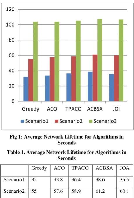
[image:3.595.314.544.67.407.2]This section is fully dedicated for analyze the simulation results of algorithms studied earlier in this paper. The main objective of this paper is to discuss the network life time, complexity and the computational time of algorithms used to solve EEC problem in WSN. From the simulation results of [1], [4] & [13] table 1 , table 2 and table 3 are made. Table 1 and fig.1 describes the average network lifetime of different algorithms suited in WSN. This average is calculated after performing simulation about 30 times and concerns different scenarios. In scenario 1 considers 100 sensors and 10 POI, scenario 2 applies 150 sensors and 10 POI and in scenario 3 200 sensors taken for 10 POIs.
Fig 1: Average Network Lifetime for Algorithms in Seconds
Table 1. Average Network Lifetime for Algorithms in Seconds
Greedy ACO TPACO ACBSA JOA
Scenario1 32 33.8 36.4 38.6 35.5
Scenario2 55 57.6 58.9 61.2 60.1
Scenario3 104 104 105.3 107.7 107
[image:3.595.318.540.582.696.2]The reason hidden in to analyze complexity and computational time in WSN is, WSN is the combination of sensors, transceivers, processors; it is the co design issue, whether to choose long battery life or high processing speed. Actually the complexity of the network system algorithm is calculated based on the number of sensors deployed, no. of agents, no. of active sensors and no. of iteration process using Big O notation. Complexity of an algorithm refers how much repetitive process going on to find result (optimal coverage) for one time slot. The need to analyze complexity is it affects the performance of the system. Table 2 and fig.2 explores maximum complexity of algorithm for one time slot.
Table 2. Complexity of Algorithms
Algorithms Big - O notations
Complexity (maximum no of iterations for one timeslot)
Greedy N2 200X30
ACO N3 100X500X30
TPACO N4 30X300X30X nkj
ACBSA N3 50X200X30
JOA N3 100X100 X 30
nk
j refers maximum value of 200
Figure 2 shows the average computational time for different algorithms discussed and it uses only 10 POIs and 100, 150 and 200 sensors respectively for scenarios.
0 20 40 60 80 100 120
Greedy ACO TPACO ACBSA JOI
32
Fig 2: Computational Time of Algorithms in Sec
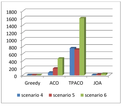
[image:4.595.315.545.71.292.2]Figure 3 shows the average computational time for various algorithms and it takes 20 POIs and 100, 150 and 200 sensors for scenarios 4, 5 and 6 respectively.
Fig 3: Computational Time of Algorithms in Sec
Figure 4 shows the average computational time for different algorithms and it has 30 POIs and 100, 150 and 200 sensors for scenarios 7,8 and 9 respectively.
Fig 4: Computational Time of Algorithms in Sec
4.
CONCLUSIONS
In this paper, different optimal algorithms used recently for EEC problem in WSN such as, ACO, TPACO, ACBSA and JOA are discussed. As an outcome, each algorithm has its unique characteristics. In greedy method, the computational time and complexity are low but network lifetime is poor. Greedy algorithm uses mathematical calculation only. Ant colony optimization algorithm is a good solution for finding shortest path between the sensor nodes but with respect to alpha and beta the entire performance of the network system will vary. Three pheromones ACO is a new approach and it removes alpha and Beta instead local & global pheromones are initialized to update activity of sensor to the base station. Probably, for small level systems in WSN having less than 200 sensors may apply TPACO algorithm for EEC problem. The ACBSA is more realistic approach, which provide longer lifetime and parameters selection was made by probabilistic sensor detection model. Result found that ACBSA is better algorithm than TPACO and ACO in network lifetime perspective. Contrary, to greedy algorithm the complexity is very high. Finally, JOI algorithm widened the view of optimal algorithm development. JOI algorithm performs based on the Jenga board game. In that, computational time is nominal and the network lifetime also better than TPACO, ACO and Greedy algorithms. As a conclusion, due to active research in WSN especially for EEC problem in future, optimal algorithms and solutions are expected and it is inevitable.
5.
REFERENCES
[1] Lee, J.-W.; Ju-Jang Lee, "Ant-Colony-Based Scheduling Algorithm for Energy-Efficient Coverage of WSN," Sensors Journal, IEEE , vol.12, no.10, pp.3036,3046, Oct. 2012
[2] Joon-Hong Seok; Joon-Yong Lee; Won Kim; Ju-Jang Lee, "A Bipopulation-Based Evolutionary Algorithm for Solving Full Area Coverage Problems," Sensors Journal, IEEE , vol.13, no.12, pp.4796,4807, Dec. 2013
[3] J. Yick, B. Mukherjee, “Wireless sensor network survey”, The International Journal of Computer and Telecommunications Networking Volume 52 Issue 12, August, 2008
0 100 200 300 400 500 600 700 800 900
Greedy ACO TPACO JOA
Scenario1 Scenario2 Scenario3
0 200 400 600 800 1000 1200 1400 1600 1800
Greedy ACO TPACO JOA
scenario 4 scenario 5 scenario 6
0 200 400 600 800 1000 1200
Greedy ACO TPACO JOA
[image:4.595.53.285.339.542.2][4] J.-W. Lee, B.-S. Choi, and J.-J. Lee, “Energy- efficient coverage of wireless sensor networks using ant colony optimization with three types of pheromones,” IEEE Trans. Ind. Inf., vol. 7, no. 3, pp. 419–427, Aug. 2011.
[5] X. Wang, G. Xing, Y. Zhang, C. Lu, R. Pless, and C. Gill, “Integrated coverage and connectivity configuration in wireless sensor networks,” in Proc. 1st Int. Conf. Embedded Netw. Sensor Syst., Nov. 2003, pp. 28–39
[6] G. Xing, X. Wang, Y. Zhang, C. Lu, R. Pless, and C. Gill, “Integrated coverage and connectivity configuration for energy conservation in sensor networks,” ACM Trans. Sensor Netw., vol. 1, no. 1, pp. 36–72, Aug. 2005.
[7] Y. Lin, X. Hu, and J. Zhang, “An ant-colony-system-based activity scheduling method for the lifetime maximization of heterogeneous wireless sensor networks,” in Proc. 12th Annu. Conf. Genetic Evol. Comput., Jul. 2010, pp. 23–30.
[8] J. Jia, J. Chen, G. Chang, and Z. Tan, “Energy efficient coverage control in wireless sensor networks based on multi objective genetic algorithm,” Comput. Math. Appl., vol. 57, nos. 11–12, pp. 1756–1766, Jun. 2009.
[9] Í. K. Altínel, N. Aras, E. Güney, and C. Ersoy, “Binary integer programming formulation and heuristics for differentiated coverage in heterogeneous sensor networks,” Comput. Netw., vol. 52, no. 12, pp. 2419– 2431, Aug. 2008.
[10]M. Dorigo and L. M. Gambardella, “Ant colony system: A cooperative learning approach to the traveling salesman problem,” IEEE Trans. Evol. Comput., vol. 1, no. 1, pp. 53–66, Apr. 1997.
[11]L. M. Gambardella, É. D. Taillard, and M. Dorigo, “Ant colonies for the quadratic assignment problem,” J. Oper. Res. Soc., vol. 50, no. 2, pp. 167–176, Feb. 1999.
[12]J. Chen, J. Li, S. He, Y. Sun, and H.-H. Chen, “Energy-efficient coverage based on probabilistic sensing model in wireless sensor networks,” IEEE Commun. Lett., vol. 14, no. 9, pp. 833–835, Sep. 2010.
[13]Joon-Woo Lee; Joon-Yong Lee; Ju-Jang Lee, "Jenga-Inspired Optimization Algorithm for Energy-Efficient Coverage of Unstructured WSNs," Wireless Communications Letters, IEEE , vol.2, no.1, pp.34,37, February 2013
[14]He, Jing; Ji, Shouling; Pan, Yi; Li, Yingshu, "Reliable and energy efficient target coverage for wireless sensor networks," Tsinghua Science and Technology , vol.16, no.5, pp.464,474, Oct. 2011
[15]Fern´an Pedraza and Andr´es L. Medaglia ‘Efficient Coverage Algorithms for Wireless Sensor Networks’