On the Absolute Sum of Chromatic Polynomial Coefficient of Graphs

(1)

Volume 2011, Article ID 271987,6pages doi:10.1155/2011/271987

Research Article

On the Absolute Sum of Chromatic Polynomial

Coefficient of Graphs

Shubo Chen

Department of Mathematics, Hunan City University, Yiyang, Hunan 413000, China

Correspondence should be addressed to Shubo Chen,[email protected]

Received 1 December 2010; Accepted 9 February 2011

Academic Editor: Dalibor Froncek

Copyrightq2011 Shubo Chen. This is an open access article distributed under the Creative Commons Attribution License, which permits unrestricted use, distribution, and reproduction in any medium, provided the original work is properly cited.

The absolute sum of chromatic polynomial coeﬃcient of forest, q-tree, unicyclic graphs, and quasiwheel graphs, are determined in this paper.

1. Introduction

For a century ago, one of the most famous problems in mathematics was to prove the

Four-Color Problem. During the period that the Four-Four-Color Problem was unsolved, which spanned

more than a century, many approaches were introduced with the hopes that they would lead to a solution of this famous problem. In 1913, Birkhoﬀ 1defined a function PM, λthat gives the number of properλ-colorings of a mapMfor a positive integerλ. As we will see, PM, λis a polynomial inλfor every mapMand is called the chromatic polynomial ofM. Consequently, if it could be verified thatPM,4>0 for every mapM, then this would have established the truth of the Four-Color Conjecture. In 1932, Whitney2expanded the study of chromatic polynomials from maps to graphs. While Whitney obtained a number of results on chromatic polynomials of graphs and others obtained results on the roots of chromatic polynomials of planar graphs, this did not contribute to a proof of the Four-Color Conjecture. Renewed interest in chromatic polynomials of graphs occurred in 1968 when Read3wrote a survey paper on chromatic polynomials. LetG be a graph and λ ∈ . A mapping f :

VG → {1,2, . . ., λ}is called aλ-coloring ofGiffu/fvwhenever the verticesuandv are adjacent inG. For a positive integerλ, the number of diﬀerent properλ-colorings ofGis denoted byPG, λand is called the chromatic polynomial ofG. By convention,PG,0 0, andPG, λ≥1 if and only ifGisλ-colorable. More precisely, we have

(2)

There are many results about the coeﬃcient of the chromatic polynomials of graphs, see related references4–8. In5, the authors characterized the absolute sum of chromatic

polynomial of trees, 2-trees, cycles, wheels and completed graphs, and obtained the sharp upper and lower bounds for the absolute sum of chromatic polynomial coeﬃcients of any connected graphs. In this paper, we investigate absolute sum of chromatic polynomial coeﬃcients of forest,q-tree, unicyclic graphs and quasiwheel graphs.

2. Preliminaries

LetG V, Ebe a graph whose sets of vertices and edges areVGandEG, respectively, n |VG|,m |EG|are the number of vertices and edges ofG.E ⊆EG, we denote by G−E_G _E_{the subgraph of}_G_{obtained by deleting}_adding_{the edges of}_E_._W _⊆ _V_G,

G−WG Wdenote the subgraph ofGobtained by deletingaddingthe vertices ofWand the edges incident with them.G·xyis the graph obtained fromGby contractingxandyand removing any loop and all but one of the multiple edges, if they arise, wherex, y ∈ VG. Terminologies and notations not defined here can be found in9. The following basic results

will be used and can be found in the references cited.

Lemma 2.1see9. iLetxandy be two nonadjacent vertices in a graphG. ThenPG, λ

PG xy, λ PG·xy, λ.

iiLete∈EG, thenPG, λ PG−e, λ−PG·e, λ.

iiiFor the empty graphOn of ordern, it is clear thatPOn, λ λn. More generally, if

Gk

i1Gi, then

PG, λ k

i1

PGi, λ. 2.1

Lemma 2.2see5. iLetG be an arbitrary graph withnvertices, then the sum of chromatic

polynomial ofPG, λ n_i1aiλiis

n

i1

ai ⎧ ⎨ ⎩

0, m / 0,

1, m0. 2.2

iiLetT be an arbitrary tree withnvertices andPT, λ _i1n aiλi λλ−1n−1. Then,

_n

i1|ai|2n−1.

iiiLetT2

nbe an arbitrary 2-tree withnvertices andPTn2, λ ni1aiλiλλ−1λ−2n−2.

Then,n_i1|ai|2·3n−2.

ivLetCn be an arbitrary graph with nvertices andPCn, λ ni1aiλi λ−1n

−1nλ−1. Then,_i1n |ai|2n−2.

vLetWnbe an arbitrary graph withnvertices andPWn, λ ni1aiλiλλ−2n−1

−1n−1_λλ₋₂_{. Then,}n

(3)

viLetKnbe an arbitrary graph withnvertices andPKn, λ ni1aiλi λλ−1λ−

2· · ·λ−n 1. Then,_i1n |ai| ni1i.

viiLetGbe an arbitrary connected graph withn(n >1) vertices andPG, λ n_i1aiλi,

then

2n−1≤

n

i1

|ai| ≤ n

i1i.

2.3

The left equality holds if and only ifG∼Tnand the right equality holds if and only ifG∼Kn.

Givenq∈, the class ofq-treesT q

n is defined recursively as follows: any complete graphKqis

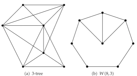
aq-tree, and anyq-tree of ordern 1 is a graph obtained from aq-treeGof ordern, wheren≥q, by adding a new vertex and joining it to each vertex of aKq inG. As an example, a 3-tree is depicted in

Figure 1(a).

Lemma 2.3see9. LetT_nqis aq-tree withnvertices, then

PTnq, λ

λλ−1· · ·λ−q 1. 2.4

Lemma 2.4see6. LetUnmis a unicyclic graph ordernand girthm, then

PUnm, λ λ−1n −1mλ−1n−m 1. 2.5

For 1 ≤ s ≤ n− 2, we denote by Wn, s the graph obtained from Wn by deleting all

but sconsecutive spokes. For convenience, we call Wn, s as the quasiwheel graphs, as shown in

Figure 1(b).

Lemma 2.5see9. LetWn, sis a quasiwheel graph withnvertices, then

PWn, s, λ λ−2s−1λ−1n−s 1 −1n−s −1n−1λλ−2. 2.6

3. Main Results

In this section, we investigate the absolute sum of chromatic polynomial coeﬃcients of forests,q-trees, unicyclic graphs, and quasiwheel graphs.

Theorem 3.1. Let F be the forest of order n and c components and PF, λ n_i1aiλi. Then

_n

i1|ai|2n−c.

Proof. It is a direct result of the combination ofLemma 2.1iiiandLemma 2.2ii.

Theorem 3.2. Let Tnq is a q-tree of ordern (n ≥ q) and PTnq, λ ni1aiλi. Then ni1|ai|

(4)

[image:4.600.184.417.92.221.2]

a3-tree b W8,3 Figure 1: The graphs 3-tree andW8,3.

Proof. We prove the result inductively onn.

inq. In this caseTnq ∼Kq.

PTqq, λ

λλ−1· · ·λ−q 1

v

i1

aiλi, 3.1

thenv_i1|ai| q_i1iq!.

iiAssume thatnkk≥q, letPT_kq, λ k_i1biλi, we haveki1|bi|q!×q 1k−q.

iiiWhennk 1, letPT_{k 1}q , λ k 1_i1 c_iλi.uis a vertex with degreeq, and the edges connectinguaree1,e2, . . . , eq, respectively. ByLemma 2.1ii, we have

PT_{k 1}q , λPT_{k 1}q −e1, λ

−PT_{k 1}q ·e1, λ

PT_{k 1}q −e1

−e2, λ

−PT_{k 1}q −e1

·e2, λ

−PT_{k 1}q ·e1, λ

· · ·

λPT_kq, λ−qPT_kq, λ

λk

i1

biλi−q k

i1

biλi.

3.2

Then,k 1_i1 |ci|ki1|bi| qi1k |bi| q 1×q!×q 1k−qq!×q 1k 1−q.

Combining above, the results follows.

Theorem 3.3. LetUnmis a unicyclic graph ordernand girthmandPUnm, λ ni1aiλi.

(5)

Proof. FromLemma 2.3, we have

PUnm, λ λ−1n −1mλ−1n−m 1

n

i0

Ci

nλn−i−1i −1m

n−m 1

i0

Ci

n−m 1λn−m 1−i−1i

m−2

i0

Ci

nλn−i−1i

n

im−1

Ci

n−1i Cn−m 1i 1−m−1i 1

λn−i_.

3.3

Letλ−1n −1mλ−1n−m 1 n_i1aiλi, then

n

i0

|ai|

m−2 i0 Ci n n im−1 Ci

n−Ci 1−mn−m 1

m−2 i0 Ci n n im−1 Cn−i

n −Cn−m 1n−i

m−2 i0 Ci n n im−1 Cn−i n − n im−1 Cn−i n−m 1

2n−2n−m 1.

3.4

Theorem 3.4. LetWn, s is a quasiwheel graph withnvertices andPWn, s, λ n_i1a_iλi.

Then,n_i1|ai|3s−12n−s 1−1−3.

Proof. FromLemma 2.5, we have

PWn, s, λ λ−2s−1λ−1n−s 1 −1n−s −1n−1λλ−2 λs−1 _{· · ·} _C1

s−1λ−2s−2 −2s−1, λn−s 1 · · · C2n−s 1λ2−1n−s−1

C1

n−s 1λ−1n−s

−1n−1λ2₋_2λ

λn _{· · ·} _C1

s−12s−2Cn−s 11 −1n−2 C2n−s 12s−1−1n−2 −1n−1

λ2

C1

n−s 12s−1−1n−1 2−1n

λ.

3.5

Letλ−2s−1λ−1n−s 1 −1n−s n_i1biλi, thenni1|bi|3s−12n−s 1−1.

Moreover,

n

i1

biλiλn · · ·

C1

s−12s−2C1n−s 1−1n−2 Cn−s 12 2s−1−1n−2

λ2

C1

n−s 12s−1−1n−1λ.

(6)

Thus,

n

i1

|bi| n

i3

|bi| C_s−11 2s−2C_{n−s 1}1 C2_{n−s 1}2s−1 C1_{n−s 1}2s−1,

n

i1

|ai| n

i3

|bi| Cs−11 2s−2C1n−s 1−1 Cn−s 12 2s−1 Cn−s 11 2s−1−2

3s−12n−s 1−1−3.

3.7

This completes the proof.

Acknowledgment

Researches are supported by the Education Bureau of Hunan Province, China Grant no. 10B015.

References

1 G. D. Birkhoﬀ, “The Reducibility of Maps,” American Journal of Mathematics, vol. 35, no. 2, pp. 115–128, 1913.

2 H. Whitney, “The coloring of graphs,” Annals of Mathematics. Second Series, vol. 33, no. 4, pp. 688–718, 1932.

3 R. C. Read, “An introduction to chromatic polynomials,” Journal of Combinatorial Theory, Series A, vol. 4, pp. 52–71, 1968.

4 H. Whitney, “Congruent graphs and the connectivity of graphs,” American Journal of Mathematics, vol. 54, no. 1, pp. 150–168, 1932.

5 N. Liu, “Research on the sum of chromatic coeﬃcients,” Operation Transactions, vol. 7, pp. 67–74, 2003 Chinese.

6 G. Haggard and T. R. Mathies, “Using thresholds to compute chromatic polynomials,” Ars

Combinatoria, vol. 58, pp. 85–95, 2001.

7 E. J. Farrell, “On the derivative of the chromatic polynomial,” Bulletin of the Institute of Combinatorics

and Its Applications, vol. 29, pp. 33–38, 2000.

8 F. Van Bussel, C. Ehrlich, D. Fliegner, S. Stolzenberg, and M. Timme, “Chromatic polynomials of random graphs,” Journal of Physics, vol. 43, no. 17, Article ID 175002, 2010.

(7)

Submit your manuscripts at

http://www.hindawi.com

Hindawi Publishing Corporation

http://www.hindawi.com Volume 2014

Mathematics

Journal of

Hindawi Publishing Corporation http://www.hindawi.com

Differential Equations

International Journal of

Volume 2014

Applied MathematicsJournal of

Mathematical PhysicsAdvances in

Complex Analysis

Journal of

Optimization

Journal of

Combinatorics

http://www.hindawi.com Volume 2014 International Journal of

Journal of

Function Spaces

Abstract and Applied Analysis Hindawi Publishing Corporation

International Journal of Mathematics and Mathematical Sciences

Hindawi Publishing Corporation http://www.hindawi.com Volume 2014

The Scientific

World Journal

Discrete Dynamics in Nature and Society

http://www.hindawi.com Volume 2014 Hindawi Publishing Corporation

Discrete Mathematics

Journal of

On the Absolute Sum of Chromatic Polynomial Coefficient of Graphs

Research Article