SIGNIFICANT PREPROCESSING METHOD IN EEG BASED EMOTIONS CLASSIFICATION

ISSN: 1992-8645 www.jatit.org E-ISSN: 1817-3195

JOIN-LESS APPROACH FOR FINDING CO-LOCATION

PATTERNS- USING MAP-REDUCE FRAMEWORK

1

M.SHESHIKALA, 2D.RAJESWARA RAO, R. VIJAYA PRAKASH

1

Research Scholar, Department of Computer Science & Engineering, KL University, Vadeshwaram,

Guntur.

2

Professor, Department of Computer Science & Engineering , KL University, Vadeshwaram, Guntur

2

Professor, Department of Computer Science & Engineering, SR Engineering College, Warangal, India

E-mail: [email protected], [email protected], [email protected]

ABSTRACT

Spatial co-location patterns represent a subset of features whose instances are frequently co-located in close proximity; For example Mountain area and new truck purchased are frequently co-located patterns, indicating that a person living close to mountainous areas is likely to buy a truck. Since the instances of spatial features are embedded in a continuous space and share a variety of spatial relationships the implementation of co-location mining can be taken as a challenge. For this, many Algorithms have been proposed, but they are prohibitively expensive with the larger data sets. We propose a parallel join-less approach for co-location pattern mining which materializes spatial neighbour relationships without any loss of the co-location instances. The parallel join-less approach drastically reduces the computation time in finding an instance look-up schema which is used for identifying co-location instances, whereas the previous join-less co-location mining algorithm finds the instances sequentially which increases the computation time. The proposed algorithm is developed on Map-Reduce. The experimental results shows the speed up in computational performance. This algorithm works well for data sets with larger size &having more number of features. As the size of the data set decreases it becomes close to the sequential approach.

Keywords: Spatial data Mining, Parallel Co-location Mining, join-less, Approach, Participation Ratio,

Participation Index, Map Reduce.

1. INTRODUCTION

The world is with Richer data, richer data with geo-location information and date and time stamps is collected from numerous sources including mobile phones, traffic, Climate events, Social Networks, GPRS tracking system, outbreaks of the diseases, various disasters, crime. This type of information is considered as important and valuable because useful patterns are generated from this data.

Spatial Data mining is the process of identifying potential useful patterns from spatial data. Usually Spatial data is stored interms of numeric values. Due to rapid growth of spatial data and use of spatial data bases such as maps, repositories of remote-sensing images, and the decennial census the application like NASA, National Institute of Justice, National Institute of Health (predicting the spread of disease), are

not supported by classical data mining techniques which needs to develop different techniques. To support this we concentrate on co-location patterns mining over spatial data bases. Basically co-location mining is the sub-domain of data mining. Co-location mining is collection of subset of features whose instances are frequently located around the geographic space.

ISSN: 1992-8645 www.jatit.org E-ISSN: 1817-3195 based on Parallel Join-less approach using

Map-Reduce framework.

One of the application domain of co-location mining is the area of identifying the location of accidents. For example, Consider a spatial data set collected from a geographic space which consists of features like Vehicles which are of different types (Cars, Buses, Auto-rickshaw, Bi-cycles, etc.,), Vehicle Parking (occasion, Place), People of different categories (Normal People, people belonging to Police Department) which is used to find why there is a crowd, whether the crowd is due to an accident or whether any Party or conference is going on, etc., This type of features are used to identify the co-located patterns to find the location of accidents.

Another application domain of co-location mining is the area epidemiology and public health. Some diseases have a high correlation to the environments in which they occur. For example, people living close to polluted areas are often more likely to get certain cancers, and people infected with Avian influenza usually live or work close to poultry and fowl habitats. The water-borne nature of Asiatic cholera mentioned above is another good example. Co-location mining can be applied to this by selecting a set of features which can potentially affect human health, treating each disease as a feature and its occurrences as instances.

Distributed execution brings in inherent properties in computing; namely speed, transparency, reliability and use of low cost commodity hardware. Hadoop distributed file system supports the distributed execution and become important open source architecture. Map Reduce programming model suits well on hadoop frameworks. In this paper we present a Map-Reduce based join-less co-location mining algorithm.

Many of the sequential steps can be parallelized by applying the map-reduce framework to join-less co-location mining, so that the computation time can be reduced without any incorrect or incomplete instances.

The remainder of the paper is organized as follows: Section 2 discusses the related work, Basic concepts of co-location mining are discussed in Section-3.In Section 4 we discuss about the major contributions where there is a scope for Parallelization and proposed Parallel Join-less co-location mining Algorithm is discussed in Section 5.Section 6 explains the implementation of Parallel Join-less co-location mining using Map Reduce framework.

Analytical Comparisons are given in Section 7 and results are discussed in Section 8.At last in Section 8 we discuss about Conclusion and Future work.

2. RELATED WORK

2.1 Space Partitioning Method

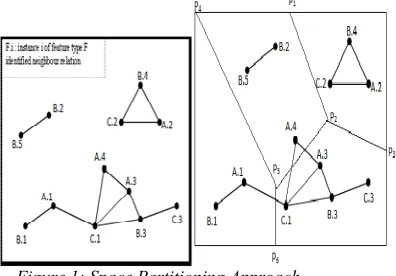
In this method [1][2]firstly, neigh-boring objects of a subset of features are identified from the given data.Refer Figure :1, the area is divided into four partitions: { ( P1,P2,P3 ) ( P1, P2, P4, P5 ) (P4, P5, P6) (

P2, P3, P5, P6) }. It finds the partition centre points

with base objects and decomposes the space from partitioning points using a geometric approach and then finds a feature within a distance threshold from the partitioning point in each area. This approach may generate incorrect co-location patterns, For example in Figure 1: it is identified that the neighboring path of co-location instance (A.4, C.1) is missing because, the instance of feature A; A.4 is falling in the partition ( P1, P2, P4, P5 ) whereas the instance of feature C; C.4

is falling in the partition ( P2, P3, P5, P6), so these

sought of co-location instances may miss across partition areas.

Figure 1: Space Partitioning Approach.

2.2 Join-Based Approach

ISSN: 1992-8645 www.jatit.org E-ISSN: 1817-3195

Figure 2 :Join-Based Approach.

2.3 Probabilistic Approach:

This approach [7] enables variation and uncertainty to be quantified, mainly by using distributions instead of fixed values in risk assessment. Identifying Table-I the distribution describes the range of possible values and shows which values within the range are most likely for figure 3. Probabilistic approach is efficient since it uses the context of uncertain data as data is collected from a wider range of data sources, but the computation time is increased since the algorithm is performed sequentially.

Figure 3: Join-based Approach

2.4 Join-Less Approach:

The join-less approach [4][5] puts the spatial neighbor relationship between instances into a compressed star neighborhood, For example in figure 4.b: the region R1, R2, R3 define the compressed star

neighborhood. Referring figure 4: all the possible table instances for every co-location pattern are generated by scanning the star neighborhood, and by 3-time filtering operation: feature-level filtering, coarse filtering and refinement filtering [5]. This join-less co-location mining algorithm is efficient since it uses an instance look-up schema instead of an expensive spatial or instance join operation for identifying co-location table instances, but the computation time is increased for 2 reasons: one is: generating co-location table instances will increase with the growing length of co-location pattern, and second reason is that

algorithm is performed sequentially. For example in figure 4 the generation of table instance for feature set{ A, B, C) are shown in figure 4.

Figure 4: Join-Less Approach

Table : I

A Sample Example Of Spatial Uncertain Data Set

Id Instance of w

Spatial

Feature Location Probability

1 A1 in Fig:1 0.2

2 A2 in Fig:1 0.4

3 B1 in Fig:1 1

4 B2 in Fig:1 0.7

5 B3 in Fig:1 0.5

6 C1 in Fig:1 1

7 C2 in Fig:1 0.3

8 D1 in Fig:1 0.2

ISSN: 1992-8645 www.jatit.org E-ISSN: 1817-3195

3.

PRELIMINARIES

In this section we discuss the basic definitions and concepts of co-location pattern mining.

3.1 Spatial Co-location Mining:

It is a group of spatial features whose instances are frequently located around the geographic space. Let F={f1, f2,……fn} be the set of features

and Z={P1, P2, ……Pn}where {P1, P2, ……, Pn}

are the subsets of features {f1, f2, …….,fn} Let T

be the threshold set {d,

min_

prev

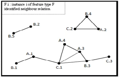
C ⋴ Z such that for C, T is valid. For example from the Figure :5 we can identify the features and instances related in a spatial data set.

Figure: 5 Example of Spatial Co-location data

From Figure:5 we identify that there are different types of features like tree, Bird, Rocks and House and we have instances for the features like trees which are of various types of trees, and Birds which are like Eagle, Sparrow, Owl, and the Features like rock and house are having only one kind of instance. From the figure we can conclude that rocks and a type of tree is co-located, Sparrow and house are co-located.

3.2 Neighborhood Relationship

Given a set of Features F, and a set of their instance objects S, and a neighbor relation R over S, a co-location C is a subset of spatial features, C

∈

the neighbor relationship i.e., (A.1, B.1)

⇒

3.3 Instance of a Feature

If we consider a set of features then there will be some associated number of objects with it. For example, if Vehicle is a feature then its associated instances are { 2-wheeler, 3- wheeler, 4 wheeler}, in general if A is a feature then its associated instance objects from the Figure: 3 are

3.4 Co-location Instance I

A co-location I is a set of objects associated in a clique instances CIk then I S, for example in

the figure the co-location instance is since is an instance feature type of is an instance feature type of B, C.2 is an instance feature type of C.

3.5 Participation Ratio

The participation ratio of feature in a co-location c is defined

For example in figure 3: the participation ratio of A with the feature B is shown in the equation (2).

3.6 Participation Index

Participation index is given as the minimum participation ratio of overall co-location features.

.

A high participation index value indicates it is highly co-located .

For example from the figure: 3, if ,

, then

The Participation ratio and Participation Index are taken as interest measures because using this measures we are able to specify which are the co-located patterns

4. OUR CONTRIBUTIONS

ISSN: 1992-8645 www.jatit.org E-ISSN: 1817-3195 1. Parallelizing the sequential join-less

co-location mining algorithm[6].

2. Implementation using Map Reduce framework.

3. Evaluation of parallel join-less co-location mining algorithm using real world data sets.

4.1 Parallelization:

The Parallelization of a sequential algorithm is a standard four step approach[8]; namely:

1. Decomposition: Splitting of sequential steps into a set of parallel steps.

2. Communication: Here communication is

needed to specify which entity communicates with which entity to perform the task.

3. Mapping: Assigning the decomposed data to

different processors that is which part is given to which processor

4. Orchestration : It is one considered as a coordinator which looks after the processors whether they are properly communicated, is there any problem with the processors and takes the proper measures, this is one which is the extra processor.

We are applying these steps to the sequential join-less co-location algorithm of [7].

4.2 The Sequential Algorithm

The algorithm of [5] is reproduced and scope of parallelization is clearly identified by the encapsulated parts in the Algorithm 1 .

4.2.1. Identifying the scope of join-less Approach where parallelism can be done:

---Algorithm 1 Join-less co-location

mining algorithm

---Inputs F= {f1,…….,fn}: a set of

spatial feature types S: a spatial dataset, R: a neighbour relationship min_prev: minimum prevalence min_cond_prob: minimum conditional probability

Output

A set of all prevalent co-location rules with participation index ≥minprev and conditional probability ≥ min_cond_prob

Variables

TD={Tf1,…., Tfn }: a set of star neighborhoods

Ck:a set of size kcandidate co-locations

SIk:star instances of size kcandidate co-locations

CIk:clique instances of size k candidate

co-locations

Pk:a set of size k prevalent co-locations

Rk:a set of size k co-location rules

Method

1)TD=gen_star_neighborhoods(F, S, R); 2) P1=F; k = 2;

3) while (not empty Pk-1) do

4) Ck=gen_candidate_co-locations(Pk-1); ----(a)

5) fori in 1 to n do

for tεTDfi where fi = cf1, cf1 is the first feature of

Ck(cf1, …….., cfn)

6) SIk=filter_star_instances(Ck,t);---(b)

7) end do

8) if k = 2 then CIk=SIk;---(c)

9) else do

Ck= select_coarse_prev_co-location (Ck, SIk,

min_prev);----(d)

10) CIk=filter clique instances(Ck, SIk);---(e)

11) end do

12) Pk=select_prev_co-location(Ck, CIk,

min_prev);----(f)

13) Rk=gen_co-location_rules(Pk,

min_cond_prob);---(g) 14) k=k+1;

15) end do

16) return⋃(R2, ……., Rk);

Referring the Algorithm 1, there is scope to execute some of the steps in a concurrent/parallel way in a distributed platform. The possible steps that can be executed parallelly are identified and explained as below:

Step a: Basically candidate co-location

generation is, finding the neighbors of each feature. Suppose { A, B, C, D, E } are the features, then candidate co-locations for size k=2 of feature A are {(A, B) (A, C) (A, D) (A, E)} and candidate co-locations for feature B are {(B, C) (B, D) (B, E)} ; candidate co-locations for C are {(C, D) (C, E)} and candidate co-locations for D are{(D,E)}. Similarly for size k=3 the candidate co-locations generated for feature A are {(A, B, C) (A, B, D), (A, B, E)} and the process is repeated for the remaining features & higher values of k with 2<=k<=(F-1),where F is the number of features.

ISSN: 1992-8645 www.jatit.org E-ISSN: 1817-3195 are number of features. Imperatively this

approach reduces the time for candidate co-locations by factorial (1/F) where ‘F’ is the number of processors used for candidate generation.

Ck=gen_candidate_co-locations (Pk-1)

Step b: In this Step Star Instance of candidate co-location from the star neighborhood are filtered. The filtering is taking place corresponding to each feature. For example; the corresponding instance neighbors for feature A with its feature set (B, C, D) are {(A1, B1) (A2, B4) (A3, B3) (A1, C1) (A2, C2) (A3, C1) (A4, C1)}.

In filtering star instances, there is scope for applying parallelism. When one processor is filtering for feature A then other processor can independently filter the star instance of the next feature and so on. This independence of star instance is explored and algorithm is modified. SIk=filter_star_instance(Ck,t);

It is to be noted that, the number of candidate co-locations examined in each star neighborhood goes on reducing by the features already considered. For example while considering filtering for B, instances of feature A need not be considered. Similarly for C, instances of A & B need not be considered. The instance filtering gets speeded up by this way of feature pruning .

Step c: When size k=2 the star instance is the clique instance. For example clique instance for feature A are{ (A1, B1) (A2, B4) (A3, B3) (A1, C1) (A2, C2) (A3, C1) (A4, C1). The same is repeated for remaining features.

Here there is scope for parallelism when one processor is returning the star instances of feature A, the other processor can return the star instances of feature B and so on. So the computation time can be reduced by (1/F) factor, where ‘F’ is the number of processors assigned for generating the clique instance.

if k=2 then CIk=SIk

Step d : For size k>2, the clique instance is generated from coarse prevalent co-location. For example the corresponding neighbors for feature A with its feature (B, C) are {(A1, B1, C1) (A2, B4, C2) (A3, B3, C1) and this is compared against minimum prevalence which is a user defined threshold; The same is with the remaining features.

Here again there is scope for parallelism, when one processor is finding the coarse prevalent co-locations for feature A, the other processor can find the coarse prevalent co-locations for B and soon. So the computation time canbe reduced by

(1/n) factorial where ‘n’ is the number of processors assigned for generating the clique instance.

Ck=select_coarse_prevalent_co-locations(Ck, SIk,

min_prev)

Step e: In this Step, clique Instances from star neighborhood are filtered when size of k>3. For suppose for feature A the clique instance with its corresponding feature (B, C ) the clique instance generated after filtering is {(A2, B4, C2) (A3, B3, C1)} the instance set (A1, B1, C1) is filtered out because there is no path between (B1, C1).

Step f: In this step prevalent co-locations are generated from candidate co-locations, clique instance and with a comparison of minimum prevalence. For Example; when k=2 the prevalent co-location generated for feature A are {[(A, B) (A,C)], [(A1, B1)(A2, B4) (A3, B3) (A1, C1) (A2, C2)(A3, C1)(A4, C1)], 0.65} and the prevalent co-locations generated for feature B are {(B, C), [(B3, C1) (B3, C3) (B4, C2)], 0.65} and the same is repeated as the size of k is increased.

Here again there is a scope for parallelism, when one processor is finding the prevalent co-locations for feature A, the other processor can find for feature B and soon. This independence of generation of prevalent co-locations is explored and algorithm is modified.

Pk=select_prevalent_co-locations (Ck,CIk,min_prev)

Step g: In this last step, generation of k-size co-locations rules(Rk) are computed by making a

comparison with the minimum conditional probability. For example; the generation of co-location rules for feature A are (A, C) when size k=2, the co-location rules for feature B is null set, correspondingly the comparisons are made against the remaining features.

Here again there is a scope for parallelism, when one processor is returning the co-locations rules for feature A, the other processor can return the co-locations rules for feature B and soon.This independence of generation of co-locations rules is explored and algorithm is modified.

Rk=gen_co-location_rules(Pk, min_cond_prob)

As identified, there is a scope for parallelism from the above explanation, we further show how it can be done in the flow chart discussed in section 4.3.

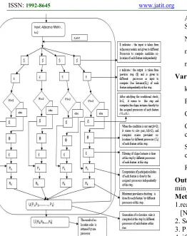
4.3 Flow-Chart of Parallel Join-less Approach

ISSN: 1992-8645 www.jatit.org E-ISSN: 1817-3195

Figure 6: A Flow chart of Parallel Join-less Approach

From the Figure : 6 the Symbols indicates the following Information.

$ = CK= generate_candidate_Co-locations

ε = SIK =filter_star_instances.

δ =( CIK=SIK)= Clique_instance=Star_instance

ф=Select_coarse_prevalent_colocation(Ck,SIK,m

in_prev)

£ = Filter_clique_instances (Ck,SIK)

Pk=select_prevalent_colocations(Ck,CIK.min_pre

v).

RK = generate_co-location_rules(Pk,min_prob)

5. THE PARALLEL JOIN-LESS

ALGORITHM

---

Algorithm-2 Input:

D= Spatial Data set.

Nf= Total Number of features in the Spatial

Data set.

Adj= Adjacency matrix computed from Spatial Data set.

NA= Number of Processors to be allotted.

min_prev=Minimum Prevalence Threshold

min_prob=Minimum Probability Threshold

Variables:

k= co-location size

Pk= a set of size k prevalent co-locations

Ck= a set of size k candidate co-locations

CIk= a set of clique instances of size k

candidates

SIk= a set of star instances of size k

candidates

Rk= a set of size k co-location rules.

Output: Co-locations satisfying min_prev and

min_prob threshold.

Method:

1.read the Number of features from the data [Nf, D]

2. Select the number of processors Nf

3. P1=F, k=2

4. if k=2 allotted number of processors NA= ( Nf-1)

5. else NA--

6. for each feature, F of (Nf-1) invite processor

‘P’ of ‘F’ do

Ck= generate_candidate_co-locations(Pk-1) by

each processor fromAdj matrix.

7. Filter_star_instance (SIk) of each feature.

SIk=filter_star_instance(Ck,t); //

8. if k=2 then SIk=CIk // assign star instance to

clique instances. 9.else do

i.Ck=select_coarse_prevalent_co-location(Ck,

SIk, min_prev)

ii. CIk=filter_clique_instance(Ck, SIk) from Adj

matrix,

10. Compute the Participation Index of each feature [based on the number of instances of each feature by its assigned processor]

Pk=select_prevalent_co-location(Ck, SIk,

min_prev)

11. Make a decision based upon minimum prevalence of each feature, if PI(F) >min_prev then goto step 12;

else goto step 13

ISSN: 1992-8645 www.jatit.org E-ISSN: 1817-3195 Rk(F)= gen_co-location_rules(Pk,min_prob) of

each feature. 13. k=k+1; 14. end do

15. gather U(R1, R2, ….., Rn) and store the

co-location result.

16. Display the co-location rules.

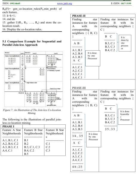
5.1 Comparison Example for Sequential and Parallel Join-less Approach

Figure 7: An Illustration of The Join-less Co-location Mining.

The following is the illustration of parallel join-less co-location mining.

PHASE I

Feature A Star Neighborhoods --- A.1, B.1, C.1 A.2, B.4, C.2 A.3, B.3, C.1 A.4, C.1

Feature B Star Neighborhoods --- B.1

B.2

B.3, C.1, C.3 B.4, C.2 B.5

Feature B Star Neighborhood s --- C.1 C.2 C.3 PHASE-II

Finding star

instances for feature

A with its

corresponding neighbors { ( B, C) }

--- A B --- A.1, B.1 A.2, B.4 A.3, B.3 A C --- A.1, C.1 A.2, C.2 A.3, C.1 A.4, C.1

Finding star instances for feature B with its corresponding neighbors { C }

--- B C --- B.3, C.1 B.3, C.3 B.4, C.2

PHASE-III

Finding star

instances for feature

A with its

corresponding neighbors { ( B, C) }

--- A B --- A.1, B.1 A.2, B.4 A.3, B.3 --- 3/4 , 3/5 --- A C --- A.1, C.1 A.2, C.2 A.3, C.1 A.4, C.1 --- 4/4 ; 2/3 ---

Finding star instances for feature B with its corresponding neighbors { C }

--- B C --- B.3, C.1 B.3, C.3 B.4, C.2 --- 2/5 ; 3/3

Figure 8: An Illustration of the Parallel join-less co-location mining.

The same process can be done for size greater than 2. To implement this algorithm we explore HDFS and Map Reduce which are the powerful open source program platforms for distributed

It is done by one Processor

It is done by one Processor It is done by one process or

ISSN: 1992-8645 www.jatit.org E-ISSN: 1817-3195 implementation.

6. MAP-REDUCE FRAMEWORK

A Programming model called as Map Reduce[8] is used for processing and generating large datasets with a parallel, distributed algorithm on a cluster. Since 1995 there in an approach called as Message Passing Interface which has both

reduce and scatter operations.

A Map Reduce job usually splits the input data-set into independent chunks which are processed by the map tasks in a completely parallel manner. The framework sorts the outputs of the maps, which are then input to the reduce tasks. Typically both the input and the output of the job are stored in a file-system. The framework takes care of scheduling tasks, monitoring them and re-executes the failed tasks.

The Map Reduce framework consists of a single master Job Tracker and one slave Task Tracker per cluster-node. The master is responsible for scheduling the jobs' component tasks on the slaves, monitoring them and re-executing the failed tasks. The slaves execute the tasks as directed by the master.

Input and Output types of a Map-Reduce job:

(input) <k1, v1> -> map -> <k2, v2> -> combine -> <k2, v2> -> reduce -> <k3, v3> (output)

7. ANALYTICAL COMPARISION

In this section, we analytically compare the proposed parallel join-less algorithm with the sequential join-less co-location algorithm[5]. First we examine the computational complexities of the two methods and then we compare each of them.

7.1 Computational Complexities

Let Tjl and Tpjl be the total

computational cost of the join-less and the parallel join-less method respectively, the following equations shows the total computation cost.

S denotes the spatial data set, denotes the cost for finding the size 2 co-location patterns in each method.

From the equation 2 and 3, there is a decrease in the computation cost for the proposed parallel join-less algorithm and it is reduced by ( 1/n ) factor for finding all neighboring pairs because, as many number of features are present, we assign those number of processors to operate in parallel.

The following are the two equations 5 & 6 used for finding the co-location patterns of size k(k>2).

(6)

is a size of k-1 prevalent co-locations set, is a size k candidate co-location set, and is a size k-candidate co-location set filtered by the coarse filtering in the sequential and parallel join-less algorithm.

In the equation (5), ,

, ,

can be ignored when compared with the other computation factors.

Comparison of computational complexities:

In this section we generate the computation cost for size 2 co-location patterns and for size k(k>2) co-location patterns for both the algorithms: For size 2 we find the computation cost of materializing neighborhoods.

Computational cost of size 2 co-location patterns:

The computation cost generated for size 2 co-location patterns of materializing neighborhood in both the algorithms is given by the following equation:

In both the methods finding the neighboring pairs cost is different. In parallel join-less the computation cost is decreased by factor for finding all the neighboring pairs.

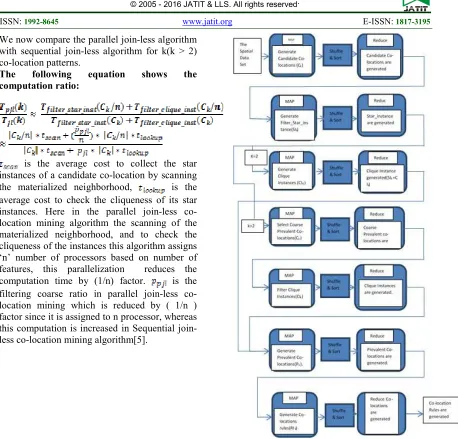
ISSN: 1992-8645 www.jatit.org E-ISSN: 1817-3195 We now compare the parallel join-less algorithm

with sequential join-less algorithm for k(k > 2) co-location patterns.

The following equation shows the

computation ratio:

is the average cost to collect the star instances of a candidate co-location by scanning the materialized neighborhood, is the average cost to check the cliqueness of its star instances. Here in the parallel join-less co-location mining algorithm the scanning of the materialized neighborhood, and to check the cliqueness of the instances this algorithm assigns ‘n’ number of processors based on number of features, this parallelization reduces the computation time by (1/n) factor. is the filtering coarse ratio in parallel join-less co-location mining which is reduced by ( 1/n ) factor since it is assigned to n processor, whereas this computation is increased in Sequential join-less co-location mining algorithm[5].

Figure :9 Map-Reduce Framework for Parallel Join-less Approach

8. EXPERIMENTAL RESULTS

ISSN: 1992-8645 www.jatit.org E-ISSN: 1817-3195 United States Board On Geographic Names [9].

The number of feature types was 92. The experiments are shown for the distances of 0.1, 0.15, and 0.2 Km, respectively. The minimum prevalence threshold was fixed to 0.3. When the neighborhood size is large, the experiment shows the computational performance of co-location mining is greatly improved with the parallel processing.

9. CONCLUSION & FUTURE WORK

In this work, we have proposed to parallelize co-location pattern mining to deal with large-scale spatial data. We have applied a distributed co-location mining algorithm on Hadoop’s Map-Reduce infrastructure. The proposed framework partitions the spatial neighborhood without any missing and duplicate neighbor relationships for co-location discovery. Each worker independently conducts the co-location mining process with a shard of neighborhood records. The co-location patterns are searched in a level-wise manner by re-using previously processed information and without the generation of candidate sets. The experimental results show that our algorithmic design approach is overall parallelizable and follows a significant increase in speed, with respect to an increase in nodes, when data size is large and the neighborhood is dense.

REFERENCES:

[1] Y. Huang, S. Shekar, and H. Xiong, ”Discovering Co-Location Patterns from Spatial Data Sets: A General Approach,” IEEE Trans. knowledge and Data Eng., vol. 16, no. 12, pp. 1472-1485, Dec. 2004. [2] Y. Huang, J. Pei, and H. Xiong, ”Mining

Co-Location Patterns with Rare Events from Spatial Data Sets,” Geoinformatics, vol. 10, no. 3, pp. 239-260, Dec. 2006.

[3] Y. Morimoto, ”Mining Frequent Neighboring Class Sets in Spatial Databases,” Proc. Seventh ACM SIGKDD Int’l Conf.

Knowledge Discovery and Data

Mining(KDD), pp. 353-358, 2001. \

[4] J.S. Yoo, S. Shekar,J. Smith, and J.P. Kumquat, ”A Partial Join Approach for Mining Co-Location Patterns,” Proc. 12th Ann. ACM Int’l Workshop Geographic Information Systems (GIS), pp. 241-249, 2004.

[5] J.S. Yoo and S. Shekar, ”A Join less Approach for Mining Spatial Co-Location Patterns,” IEEE Trans. knowledge and Data Eng.(TKDE), vol. 18, no. 10, pp. 1323-1337, Dec. 2006. [5]

[6] L. Wang, Y. Bao, J. Lu and J. Yip, ”A New Join-less Approach for Co-Location Pattern Mining,” Proc. IEEE Eighth ACM Int’l Conf. Computer and Information Technology (CIT), pp. 197-202, 2008. [7] L. Wang, P. Wu, and H. Chen, ”Finding

Probabilistic Prevalent Co-locations in Spatially Uncertain Data Sets,” IEEE Trans. knowledge and Data Eng.(TKDE), vol. 25, no. 4, pp. 790-804, Apr. 2013.

[8] Tom White, “Hadoop , The definitive Guide”,O’REILLY, ISBN: 978-93-5023-756-4, May.2012.