M E T H O D
Open Access
MUSIC: identification of enriched regions
in ChIP-Seq experiments using a
mappability-corrected multiscale signal
processing framework
Arif Harmanci
1,2, Joel Rozowsky
1,2and Mark Gerstein
1,2,3*Abstract
We present MUSIC, a signal processing approach for identification of enriched regions in ChIP-Seq data, available at music.gersteinlab.org. MUSIC first filters the ChIP-Seq read-depth signal for systematic noise from non-uniform mappability, which fragments enriched regions. Then it performs a multiscale decomposition, using median filtering, identifying enriched regions at multiple length scales. This is useful given the wide range of scales probed in ChIP-Seq assays. MUSIC performs favorably in terms of accuracy and reproducibility compared with other methods. In particular, analysis of RNA polymerase II data reveals a clear distinction between the stalled and elongating forms of the polymerase.
Background
With the recent advancements in sequencing technologies, chromatin immunoprecipitation (ChIP)-based enrichment of DNA sequences followed by sequencing (ChIP-Seq) [1,2] has become the mainstream experimental method for genome-wide measurement of the locations of DNA binding proteins like transcription factors (TFs) and post-translational modifications of histone proteins, or histone modifications (HMs) [3,4]. Consortium projects such as ENCODE [5] and the Roadmap Epigenomics Project [6] generated ChIP-Seq datasets to map the chromatin states of many cell lines and tissues [7]. These substantially increased the number of publicly available ChIP-Seq datasets for a diverse set of HM and TF binding profiles. Following sequencing, it is necessary to computationally process the read depth (RD) signal profile to identify the enriched regions (ERs) across the genome [8].
Depending on the target of the ChIP-Seq assay, the length scale of ERs can vary extensively for different ex-periments, which changes the ER identification workflow.
For TF binding, for example, the ERs are observed at punctate regions of protein binding and are hundreds of nucleotides in length [9]. For most HMs, ERs are broad. For example, the ERs for the repressive heterochromatin mark H3K9me3 can extend up to a few megabases. An-other interesting example is RNA polymerase II (Pol2), which binds to promoters and gene bodies for the pur-pose of mRNA transcription and whose ERs can extend over the whole gene bodies or can be punctate and concentrated close to gene promoters. Development of efficient computational methods for identification and characterization of the broad ERs is necessary for under-standing the regulatory effects of HMs and diffuse DNA binding proteins on gene expression as increasing evi-dence indicates that these epigenetic factors are major driving factors in pluripotency [10] and of disease mani-festation, such as cancerogenesis [11-15].
There are two main challenges for identification of broad ERs. First, unlike ERs for TF binding, broad ERs are observed at longer length scales and the length spectrum of ERs is broad for many HMs. This makes it necessary to identify the ERs at different scales. A widely used method for identifying ERs in HM signal profiles involves smoothing the signal profile with a kernel of constant size and shape and using a null model (for * Correspondence:[email protected]
1
Program in Computational Biology and Bioinformatics, Yale University, 260 Whitney Avenue, New Haven, CT 06520, USA
2
Department of Molecular Biophysics and Biochemistry, Yale University, 260 Whitney Avenue, New Haven, CT 06520, USA
Full list of author information is available at the end of the article
example, a Poisson or negative binomial) to identify the significantly enriched regions. It is, however, not clear how the kernel size and shape should be selected. The multiscale approaches proposed by the wavelet-based methods address this issue, although the reasoning and motivation for which wavelet functions are used in these methods are generally not well established.
Second, the signal profiles contain systematic noise introduced into the RD signal by repeat regions with low mappability [9,16], in the form of loss of signal. This noise causes discontinuities in the identified ERs. This is an important factor, especially in intergenic regions where a large ER, which may mark a long regulatory region, is fragmented into smaller ERs.
Many different approaches have been applied for identification of broad ERs, including change point identification within the formality of Bayesian inference (BCP [17]), local island identification and clustering (SICER [18]), local thresholding and merging (MACS), using local Poisson statistics to identify broad ERs (SPP), and wavelet-based smoothing and identification of ERs (WaveSeq [19]), which is also applied to analysis of ChIP-chip datasets [20].
In this paper, we present MUSIC, a method to identify ERs in ChIP-Seq experiments. MUSIC first uses mappabil-ity correction at nucleotide resolution to correct for the spurious loss of signal in regions with low mappability. Next, MUSIC performs a multiscale decomposition of the corrected RD signal. This decomposition is adopted from the scale-space filtering theory in signal processing [21], which is used widely for signal segmentation, smooth-ing, and enhancement. Unlike the wavelet-based multi-scale approaches that use linear filtering, we take an approach to multiscale decomposition that uses non-linear median filtering. Basically, MUSIC exploits the fact that, at each decomposition, smoothing with a cer-tain window length removes small details in the signal (like small peaks and small valleys) and the candidate ERs in the signal are detected as regions between con-secutive local minima of the smoothed signal [22,23]. MUSIC then identifies the significantly enriched re-gions at each scale, which yields the scale-specific ERs (SSERs). In general, SSERs at smaller scales correspond to more punctate binding/modification levels compared with SSERs at higher scales, which represent broader ERs. To identify the final set of ERs, MUSIC merges the SSERs from all the scales.
In order to evaluate the accuracy of the ERs identified by MUSIC, we performed benchmarking experiments to compare the accuracy and reproducibility of the ERs identified by MUSIC with numerous other ER identifi-cation methods. We concentrated on factors whose ERs manifest at different (that is, broad, puncate, and point binding) length scales so as to make a thorough
comparison with a variety of accuracy metrics. We show that MUSIC performs favorably in the comparisons. Next, we concentrate on the Pol2 ChIP-Seq datasets. Motivated by the basic observation that the stalled poly-merase tends to show punctate enrichments (SSERs at small scales) and that elongating polymerase tends to show broad enrichments (SSERs at higher scales), we computed the SSERs for the Pol2 ChIP-Seq dataset using MUSIC. Using the identified SSERs, we then estimate the length scale for polymerase binding for all protein coding genes. We demonstrate that the genes with punctate poly-merase binding have significantly lower expression (close to 0) than the genes that show more broadly bound poly-merase. We corroborate this observation with the ChIP-Seq data for the elongating (phosphorylated) form of Pol2. We conclude that the length scale of binding of polymer-ase at gene promoters as identified by MUSIC is indicative of its state, that is, stalled or elongating.
The paper is organized as follows. We first present the MUSIC algorithm and lay out the steps of the algorithm. Then we present a comparison of MUSIC with other ER identification algorithms. We finally present the analysis of the Pol2 data with gene expression levels.
Results and discussion
MUSIC algorithm
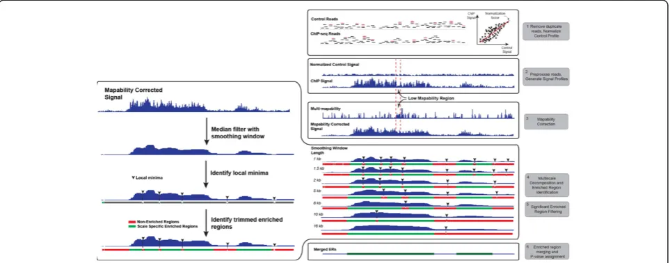
Figure 1 shows a flowchart for MUSIC (see Materials and methods for more details). Here we summarize each step briefly. The input to MUSIC comprises the sets of reads from the ChIP and control samples (steps 1 and 2), the set of window lengths to be used in multiscale decomposition, and the multi-mappability profile. The multi-mappability profile quantifies, at each position, the average number of reads that get mapped non-uniquely (see Materials and methods). Therefore, for a position that is uniquely mappable, the multi-mappability value is 1. For repeat regions, the multi-mappability value increases. Figure S1 in Additional file 1 shows the aggrega-tion of multi-mappability profiles around different gen-omic elements for different read lengths. It should be noted that the multi-mappability signal is computed once for each read length (see the 'Multi-mappability signal generation' section in Materials and methods). MUSIC first preprocesses the reads and filters the duplicates, then computes a scaling factor using linear regression between the ChIP and control signal profiles (see the 'Input normalization' section in Materials and methods). The slope of the regression is used as a normalization factor for control.
correction filter' section in Materials and methods). The correction can be formulated as:
x˜i¼max½xi;|fflfflfflfflfflfflfflfflfflfflfflfflfflfflfflfflfflfflfflfflfflfflfflfflfflfflfflfflfflfflfflfflfflfflfflffl{zfflfflfflfflfflfflfflfflfflfflfflfflfflfflfflfflfflfflfflfflfflfflfflfflfflfflfflfflfflfflfflfflfflfflfflffl}medianðfxaga∈½ilc=2;iþlc=2jma<mexonicÞ Median of the signal values at highly mappable
position aroundi
zfflfflfflfflfflfflfflfflfflfflfflfflfflfflfflfflfflfflfflfflfflfflfflfflfflfflfflfflfflfflfflfflfflfflfflfflfflfflfflfflfflfflfflffl}|fflfflfflfflfflfflfflfflfflfflfflfflfflfflfflfflfflfflfflfflfflfflfflfflfflfflfflfflfflfflfflfflfflfflfflfflfflfflfflfflfflfflfflffl{ Maximum of the signal value atiand
the median signal at highly mappable positions
where xi and ~xi are the uncorrected and corrected signal values, respectively, at positioni,mais the value of multi-mappability profile at position a, lc is the length of the median filter utilized in correction, which is by default set to 2,000 bp, andmexonic is the average
multi-mappability signal value over the exonic regions, which we identified as the most mappable regions in the genome (Figure S1 in Additional file1). In summary, for each position i, MUSIC computes the median of the signal values at highly mappable positions (multi-mapp-ability signal smaller than mexonic) within lc vicinity of
i. Then MUSIC compares this value with the signal value at i and assigns the maximum to the corrected value. The basic idea behind this correction is that since we know that low mappability causes a decrease in the signal level, if the signal value atiis higher than its vicinity, then it is highly likely that the mappability did not affect the signal value ati. Otherwise, it is replaced by the median signal value at mappable positions. The maximum filtering, also known as dilation in the image
processing literature, is used for feature enhancement in images [24], which also enables MUSIC to enhance the ERs for easier identification. It should be noted that the mappability correction is not required for correcting the signal profiles of very punctate signal profiles like TFs since TF peaks in the signal profile have predominantly single summits, which do not get segmented by regions with low mappability.
MUSIC then performs median filtering to the mappability-corrected ChIP profile to compute multiscale decompos-ition of the ChIP signal at multiple length scales (step 4 in Figure 1; Figure S2 in Additional file 1; 'Multiscale decom-position by median filtering' section in Materials and methods). For this, MUSIC uses window lengths begin-ning with lstart and ending at lend and performs sliding window-based median filtering. The window length is in-creased multiplicatively between consecutive scales; thus, the window lengths form a geometric series:
lstart;lstartσ;lstartσ2;⋯;lend
where σ is the multiplicative factor between consecu-tive window lengths, which is set to 1.5 by default.
⌊lstart×σ⌋denotes the largest integer value that is smaller
thanlstart×σ, which is necessary since the window lengths
[image:3.595.58.540.90.279.2]are integer values. The multiplicative factor tunes how finely MUSIC samples the scale spectrum. For small σ, MUSIC analyzes large numbers of scale lengths, although this also increases the run time.
For smoothed signal at each scale, MUSIC identifies all the local extrema, that is, local minima and local maxima (step 4 in Figure 1; 'Identification of candidate scale-specific enriched regions' section in Materials and methods). The regions between the consecutive local minima are marked as the candidate ERs. Due to the nature of the smoothing process, the signal may become oversmoothed at large scales (long windows), which causes over-merging of the ERs. To avoid this, it is necessary to remove the regions with over-smoothed signal. For each ER, MUSIC computes the fraction of the maximum of smoothed RD signal (at the corresponding scale) to the maximum of the unsmoothed ChIP signal within the boundaries of the ER. If this fraction is smaller than the smoothed versus unsmoothed signal ratio thresh-old (denoted byγ), MUSIC discards this candidate ER (see the 'Comparison of smoothed signal in candidate enriched regions' section in Materials and methods).
The regions identified from the consecutive minima are rough and it is necessary to identify the location of the densest signal enrichment within each region. To achieve this, MUSIC performs a Poisson background-based thresholding and P-value minimization to trim the ends and identify the densest regions of signal en-richment in the ERs. Step 5 in Figure 1 illustrates the trimmed ends of the candidate ERs. Finally, MUSIC
computes the P-value from a binomial test for each
trimmed region and filters out those whose P-values are larger than 0.05. We refer to the remaining regions as scale-specific enriched regions; these contain all the information about the enrichments in the signal over a spectrum of length scales (see the 'Candidate enriched region end trimming using a Poisson distribution model' and 'Candidate enriched region end trimming via P-value minimization' sections in Materials and methods).
Identification of enriched regions
MUSIC utilizes SSERs to identify ERs in the genome. For this, the candidate ERs are computed by merging the SSERs identified in all the scales (step 6 in Figure 1). MUSIC then filters out the ERs with respect to discord-ance of the signal levels on positive and negative strands. For this, MUSIC computes the amount of signal mapping to the positive and negative strands in each ER and filters out the ERs for which the counts of reads that map to the positive and negative strands are within a factor of 2 of each other (see the 'Per strand concordance test' section in Materials and methods).
For each of the remaining ERs, MUSIC computes the P-value from a binomial test using the number of reads in the ChIP and normalized control samples. The multiple hypothesis correction is performed by the Benjamini-Hochberg procedure [25]. The q-values
computed after the correction are thresholded with respect to 0.05 for identification of the significant ERs (see the 'P-value computation and false discovery rate estimation' section in Materials and methods). For each ER, MUSIC also computes a summit (see the 'Summit and trough identification' section in Materials and methods) and a trough in the ER. The summits repre-sent the point of strongest binding/modification in the ER and troughs represent the point where there is a depletion of signal, which may represent the nucleosome-free re-gions. Finally, in order to visualize the processed tracks, MUSIC has an option to save the smoothed signal profiles at each decomposition scale in bedGraph format, which can be loaded to a genome browser.
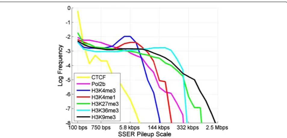
SSER pileup scale and evaluation of broadness of enrichment
The scale dependence of SSERs is a useful property for evaluating the broadness of enrichment. Each SSER rep-resents a local ER at a certain length scale. Therefore, the signal around a position that is covered by a large number of SSERs (at different scales) is more broadly enriched than the signal around a position that is covered by fewer SSERs. Following this basic observation, MUSIC pools the SSERs from all the scales and counts the num-ber of SSERs covering each position, which quantifies the broadness of enrichment at each position in the genome. We refer to this value as the SSER pileup scale of the position.
Additional file 1 shows the scale spectrum for a more extensive list of HMs with corresponding length scales. Finally, the Pol2 signal profiles show a high frequency of enrichments at small scales that gradually decreases as the scale increases.
Comparison with other methods
In order to evaluate the accuracy of the ERs, we compared MUSIC with eight other algorithms that identify ERs from ChIP-Seq data: DFilter [26], ZINBA [27], F-Seq [28], BCP [17], SPP [29], MACS [30], SICER [18], and PeakRanger [31]. A detailed list of the parameters used to run each method are presented in the 'Parameter selection for benchmarking' and 'Parameters used for peak calling methods in benchmarking' sections in Materials and methods.
Comparison of broad enriched region identification
To compare the performance of the methods on broad marks, we ran all the algorithms (in broad ER identifica-tion mode) using H3K36me3 and H3K27me3 ChIP-Seq datasets for GM12878 and K562 cell lines from the ENCODE project [5]. H3K36me3 is known to mark the bodies of actively transcribed genes [32]. We used this observation to build a gold standard set for H3K36me3 comprising the bodies of expressed transcripts. We downloaded the transcript quantifications (in Reads Per Kilobase per Million mapped reads, RPKM ) from Djebali et al. [33] and removed transcripts with low expression. The bodies of the expressed transcripts were then merged to generate the gold standard set for
H3K36me3 ERs. Rather than selecting one expression threshold for identifying the expressed transcripts, we selected thresholds between 0 and 1 RPKM increasing in steps of 0.01 so as to evaluate the accuracy of ER calls against multiple gold standard sets identified at different levels of gene expression.
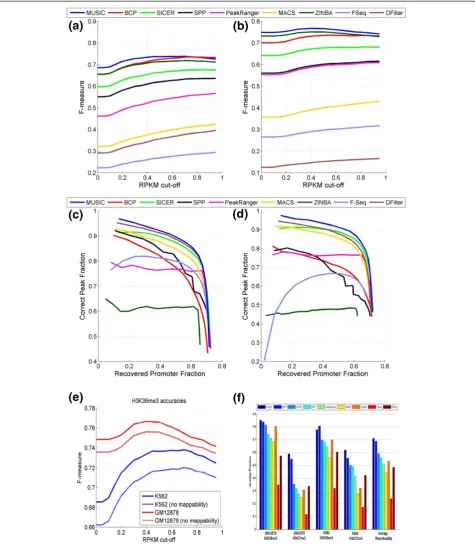
We observed that MUSIC tends to identify longer ERs compared with other methods and that different methods have very different total ER coverage. To measure the ac-curacy of identified ERs, it is necessary to account for the difference in the coverage of the identified ERs. We used sensitivity (the fraction of the coverage of correctly pre-dicted ERs to the coverage of the gold standard set) and positive predictive value (the fraction of the coverage of correctly predicted ERs to the coverage of identified ERs). To summarize these accuracy values in one measure, we chose the F-measure, which is computed as the harmonic mean of sensitivity and positive predictive value (see the 'Parameter selection for a new ChIP-Seq dataset' section in Materials and methods). Having one measure of accur-acy enables us to easily compare the accuraccur-acy of methods with changing RPKM thresholds.
[image:5.595.60.537.87.316.2]mappability correction and computed the F-measure of the ERs. Figure 3e shows the F-measure versus RPKM threshold. Using a mappability map significantly increases
[image:6.595.61.537.89.636.2]the accuracy of the identified ERs for H3K36me3 and shows the importance of utilizing the mappability correc-tion in ER identificacorrec-tion.
Figure 3Accuracy comparison for predicted H3K36me3 ERs. (a,b)F-measure versus RPKM threshold for H3K36me3 ERs for GM12878(a)and K562(b)
We also evaluated the reproducibility of the ERs. For this comparison, we used the replicates generated by the ENCODE project. For H3K36me3 and H3K27me3, we computed the reproducibility as the average of the frac-tion of the overlapping regions to the total coverage of each replicate (see Materials and methods; Figure 3f ). The overall reproducibility for MUSIC is higher than that for the other methods and MUSIC has the best or the second best reproducibility compared with the other methods.
Comparison of punctate enriched region identification
While the multiscale approach developed in MUSIC is most applicable to identifying ERs over a range of length scales, it can be applied to the identification of punctate ERs, such as for TFs. To compare the methods listed above in the identification of punctate ERs, we first chose to compare the methods on the H3K4me3 HM, which marks the promoters of active genes. We utilized the promoters of the active genes (RPKM >0.5) as gold standard positives. We identified ERs that have at least 5% overlap with the promoter region (2 kb region around the annotated transcription start site). For this comparison, we sorted the top 20,000 ERs with respect to the score reported by each method then computed the overlap of the ERs with active promoters. Starting from the top ERs, we plotted fraction of active pro-moters that are identified correctly versus fraction of ERs that overlap with active promoters. These are shown in Figure 3c,d, respectively, for the K562 and GM12878 cell lines. MUSIC performs favorably compared with the other methods, followed by DFilter and SICER. We also compared these methods using the TF CTCF via the enrichment of the known CTCF binding motifs. In this comparison, MUSIC is among the best performing methods (Table S2 in Additional file 1; 'Parameter se-lection for a new ChIP-Seq dataset' section in Materials and methods).
Analysis of the RNA polymerase II and gene expression levels
Next, we concentrated on the Pol2 binding data from the ENCODE project. Pol2 shows distinct patterns of binding depending on the state of polymerase, that is, genes with broadly bound polymerase are being actively transcribed (elongating Pol2) and show higher levels of expression compared with genes that are bound in a punctate fashion by Pol2 (stalled Pol2) [34,35]. This makes the Pol2 data suitable for multiscale analysis using MUSIC.
To evaluate the relation between the expression and the length scale of binding, we processed Pol2 ChIP-Seq data for the K562 cell line from the ENCODE project using MUSIC and computed the SSER pileup scale using
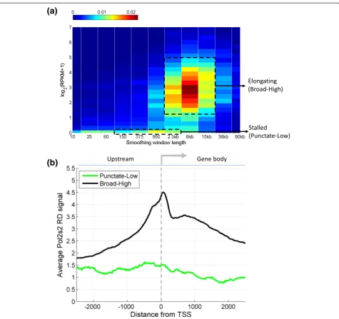
parameterslstart = 10 bps,lend= 2.5 Mbps, and σ= 1.5. Then, for each protein coding gene, we assigned the broadness of Pol2 binding as the maximum of the SSER pileup scale within the gene body. We then quantified the gene expression levels in RPKM using the RNA-Seq datasets from the ENCODE project. Finally, we plotted the two-dimensional histogram of binding scale and gene expression level for each gene (Figure 4a). In the plot, two components are revealed. One component is at low log expression levels (<0.1) and has a maximum frequency at a scale length of 950 bp. This component corresponds to stalled Pol2, which has a punctate enrich-ment profile and produces very little or no transcripts. The second component is observed at log RPKM <0.5 with a peak of scale level at around 6 kilobases. With the elongating Pol2 and high expression levels, this compo-nent is associated with actively transcribed genes.
To study these components further, we focused on the two components of polymerase binding and gene expres-sion levels. For the genes with stalled polymerase, we selected genes with a pileup scale between 150 bp and 2.3 kbp and low expression (log(RPKM) <0.1). For the genes with elongating polymerase, we selected genes with a pileup scale >950 bp with high expression (log (RPKM) >0.1). We performed aggregation of the ChIP-Seq RD signal for the elongating form of polymerase, Pol2s2, from the ENCODE project, around the promoters of genes in both sets. The motivation is that signal for Pol2s2 marks the location of elongating polymerase, which should asso-ciate with the promoters that we marked as elongating and not with the promoters that are bound by the stalled polymerase. Figure 4b shows the aggregation plots. As ex-pected, for the punctate bound and low expression genes, the aggregation plot shows very little Pol2s2 binding. In contrast, the high expression and broad bound promoters show substantially higher Pol2s2 binding that extends into the gene body.
Conclusions
filtering. With the diverse enrichment characteristics of the targets for ChIP-Seq experiments, we believe this customizability will prove very useful for process-ing datasets generated usprocess-ing ChIP-Seq experiments for which broad binding profiles are observed.
Compared with kernel-based linear filters (which are also used in wavelet-based multiscale decompositions), multiscale decomposition using median filtering has two advantages [36]. First, at low noise levels, median smoothing preserves the edges - that is, the sharpness of the increase and decrease of the RD signal at the ends of ERs - in the signal better than linear filters. Second,
[image:8.595.61.537.86.533.2]in a post-processing step after representation is com-puted, unlike MUSIC, where the mappability correction is performed before decomposition is computed.
We also processed Pol2 data using MUSIC. Pol2 is suitable for multiscale analysis because, unlike other DNA binding proteins, it shows a wide spectrum of ER lengths. Furthermore, the broadness of binding of Pol2 is indicative of its state, that is, stalled or elongating. We showed that there is a significant distinction between the expression levels of genes that are bound broadly by Pol2 compared with genes that are bound in a punctate fashion.
Materials and methods
We describe the signal processing methodology underlying MUSIC in more detail.
Input normalization
It is necessary to normalize the control signal profile with respect to the ChIP-Seq profile because the RDs can be different. For each chromosome, MUSIC first di-vides the chromosome into 10,000 bp bins then com-putes the total ChIP-Seq and control signal in each window. Finally, it estimates the normalization factors as the slope of the minimum squared error estimate of the slope:
ρ¼argmin ρ0
X
i
wi−ρ0⋅ci
ð Þ2
( )
where wi and ci represent the total signal in the ith bin for ChIP and control samples, respectively. The normalization procedure aims to match the background signal level in the ChIP sample to the control sample.
Mappability correction filter
Given the read depth signal at each nucleotide position, MUSIC corrects for the loss of signal caused by low mappability using the following filtering:
~
xi¼ max xi; median f gxa a∈½i−lc=2;iþlc=2jma<mexonic
h i
where xi is the signal value at nucleotide position i, median({xi}) is the median of the set {xi},mais the value of the multi-mappability profile at position a, and lc is the window length used in mappability aware filtering. Using this filtering, MUSIC infers the signal values for positions with low mappability using the median of the values at nearby positions with a multi-mappability sig-nal lower than mexonic, which is 1.2. We selected this
value since it is the smallest multi-mappability signal profile value, that is, the most mappable, over exons and promoters as shown in Figure S1 in Additional file 1. We set the window length lc to 2,000 bp empirically.
This window length depends on the distribution of length of the non-mappable region lengths. Different lc values did not seem to have a significant effect on the results for the human genome.
This filtering procedure is inspired by the dilation oper-ation in image processing, which is a morphological filter and has been used, in combination with other filters, for image enhancement. In our experiments, we also observed that the operation defined above tends to enhance the sig-nificant ERs.
Multiscale decomposition by median filtering
MUSIC utilizes median filtering-based multiscale decom-position. We selected to use median filtering since it has many applications in signal processing for performing sig-nal smoothing with edge preserving. Given a window length, that is, the scale, median filtering can be formu-lated as:
xsi¼median f g~xa a∈i−ls
2;iþls2
½
;ls∈lstart;lstartσ;⋯lend where xs
i is the i
th
value of the decomposition at scale levelsfor which the smoothing window length isls, and ~
xis the mappability corrected signal profile. The window length lsis chosen from a geometric series with the fac-tor σ to ensure that the larger scales do not dominate the identified SSERs [21].
The multiscale decomposition enables automatic iden-tification of blobs in the signal profiles at different scales with very small computational requirement. MUSIC uses a fast and efficient method to implement the median filtering by storing the histogram of the signal values in the current window and processing only the new and obsolete signal values that enter and leave the current window to update the histogram when moved to the next window.
Identification of candidate scale-specific enriched regions After the multiscale decomposition, MUSIC identifies all local minima in the decomposition. MUSIC utilizes regions between minima points as the regions of enrichment. For this, MUSIC computes the derivative of the signal at each point as the difference between consecutive values:
x0si¼ xs i−xsi−1
where x0is is the derivative of the smoothed signal xsi. MUSIC assigns the local extrema at the points where the derivative changes sign:
Imin¼ fi x0si < 0; x0si−1 > 0 Imax¼ i x0si > 0; x
0s
i−1 < 0
candidate ERs of xs
i are identified as the regions between the consecutive minima.
Comparison of smoothed signal in candidate enriched regions
For the candidate ERs in each smoothing scale, MUSIC uses the value of smoothed signal levels and unsmoothed signal levels for assessing the quality of the ERs. A scale-specific candidate ER is filtered if the ratio of the maximum of the smoothed signal to the maximum of the unsmoothed signal within the candidate region is higher than the smoothing statistic threshold, γ. In other words, MUSIC removes the candidate ER [i,j] at scalesif:
max xs a a∈½ i;j
max f gxa a∈½ i;j
<γ:
The comparison between the ratio on the left and γ
offers a simple and efficient check to evaluate whether the signal within the candidate region identified at the scale levelsis severely smoothed. This way, MUSIC effi-ciently detects and avoids over-merging of consecutive regions that have high signal enrichment and are close to each other. We analyzed the significance of SSERs versusγand determined that a default value of 4 enables a conservative list of SSERs (see the 'Selection ofσ' section in Materials and methods).
Candidate enriched region end trimming using a Poisson distribution model
MUSIC trims the ends of the candidate ERs using a Poisson null model for the signal distribution. For this, MUSIC divides the genome into 1 Mbp windows and for each 1 Mbp window estimates the mean of all the values. Using this as the mean parameterμof the Poisson distribution, MUSIC selects a threshold that satisfies a 5% false positive rate:
τ¼argmin t
FXμð Þt >0:95
; XμePoissonð Þμ
where FXμ represents the cumulative distribution func-tion ofXμ, which is distributed as Poisson with meanμ.
For a region with start and end at positions i and j, respectively, the trimmed end coordinates are given as:
i′¼ argmin
a ðxa > τÞ; a∈½ i;j
j′¼ argmax
a ðxa > τÞ; a∈½ i;j
where i′and j′are the trimmed start and end coordi-nates, respectively. The regions for which the signal level does not pass the threshold are removed from the candidate ER list.
Candidate enriched region end trimming viaP-value minimization
MUSIC fine-tunes the ends of the merged ERs using a
P-value minimization procedure. This maximizes the
compactness of the merged regions. The end-refined merged regions are the candidate regions of enrichment before P-value computation. The end trimming can be formulated as:
i′¼ argmin
a p a; jjlpval ¼ðj−aþ1Þ
; a∈½ i;j j′¼ argmin
a p i
′; ajlp
val ¼ a−i 0þ1
ð Þ
; a∈½i0;j where p a ;b lp valÞ represents theP-value for the region starting at aand ending at b with the length ofP-value window given bylpval(Refer toP-value computation).
Per strand concordance test
For each ER, MUSIC computes the total signal on posi-tive and negaposi-tive strands and filters out the ERs for which there is high discordance between the signals:
min
X
i xþi
X
i x−i ;
X
i x−i
X
i xþi
0 B B @ 1 C C A<0:5
whereX
i
xþi andX i
x−i is the total signal on the positive
and negative strand within the start and end coordinates of the ER, respectively.
P-value computation and false discovery rate estimation We use one-tailed binomial test to compute theP-values for each candidate ER. We first count the number of reads in the chip sample (nchip) and control sample (ncontrol) that overlap with the region, then compute one tailedP-value as:
p¼ X
n0chipþn0conrol
r¼n0chipþ1
n0chipþn0control r
0:5 n 0
chipþn
0
control
where n0chip and n0control are the normalized read counts for the region:
n0chip¼nchip lchip lpval
n0control¼ncontrol lcontrol
lpval
Materials and methods). We perform multiple hypoth-esis correction by false discovery rate (FDR) estimation (q-values) using the Benjamini-Hochberg procedure [25]:
qi¼pi NERs
i
whereNERsis the total number of ERs andi is the rank of the ER in the ER list sorted with respect to increasing P-value. By default, MUSIC uses a default q-value cutoff of 0.05. The filtered ERs are reported in BED format with their q-values in the score field.
Summit and trough identification
For DNA-binding protein ChIP-Seq data, for example, TFs, MUSIC reports the location of the highest signal level within the ER as the summit of the signal, which can be used as the binding position. An important con-sideration in ER identification is the identification of valleys (or troughs) in the signal. For example, the troughs in H3K4me3 and H3K27ac ERs may correspond to the nucleosome-free regions in promoters and enhancers, respectively, where the TFs can interact with DNA and regulate transcription. Therefore, identification of the troughs (in addition to the summits) is an important piece of additional information for each ER. Our analysis, how-ever, shows that many of the troughs in ChIP-Seq signals are caused by a decrease in the mappability of the genome (Figure S6 in Additional file 1). MUSIC reports one trough position in each peak by determining the smallest position within the top two tallest peaks such that the average multi-mappability around the trough is smaller than the exonic multi-mappability (me). No troughs are reported if there is only one summit in the ER.
Multi-mappability signal generation
MUSIC can generate multi-mappability signal profiles. For this, MUSIC utilizes an existing read mapping tool. Currently MUSIC uses bowtie2 [40], a very popular short read mapping algorithm, by default. MUSIC first fragments all the chromosomes to the read length of interest, maps all the fragments to the genome using bowtie2 with two mismatches and reporting of a max-imum of the top five multimapping positions per frag-ment. Then MUSIC uses the mapped reads to build the multi-mappability RD signal profile. The regions with high signal correspond to regions with low mappability. We generated multi-mappability profiles for the hg19 genome assembly for read lengths of 36, 50, 76, and 100 bp, which are available for download with MUSIC.
Parameter selection for benchmarking
Several parameters are associated with MUSIC. We discuss the general selection procedure for these, which can be used as guidelines when running MUSIC.
Selection of lbeginand lend
For selectinglbeginand lend, we utilize a basic property of median filtering (Figure S3 in Additional file 1). In order to detect an enrichment of length l it is necessary to ensure:
lbegin<2l
Similarly, in order to distinguish between two ERs that arel base pairs away from each other, it is necessary to ensure:
lend <2l
Thus,lbeginshould be small enough to ensure detection of the smallest enrichments that we expect to observe and lendshould be set to a value to detect each individual en-richment separately without over-merging (Figure S3b,c in Additional file 1). As we assume that the basic enriched units are the gene bodies, we chooselbeginusing the length distribution of gene bodies (Figure S3e in Additional file 1). As most of the genes are longer than 512 bp (log value of 9), we setlbeginto 1,000 bp. For choosing lend, we computed the cumulative distribution of gene-gene distances (Figure S3d in Additional file 1). Evaluating this plot, we observe that a 10% cutoff occurs at around a log distance of 12.5. As a suitable compromise with the gene length distribution (the median is at a log value of 15), we setlendto 2 × 213≈16,000 bp. For punctate marks (like H3K4me3 and H3K27ac), MUSIC is set to run at a smaller scale spectrum than for broader marks using lbegin= 100,lend= 2,000. This way MUSIC aims to identify small ERs and to identify enrichments at the expected length range of several kilobases. For TFs, where the bind-ing events occur at almost sbind-ingle base pair resolution, MUSIC is set to run at very small scales withlbegin= 100, lend= 200. It is worth noting that the multiscale decompos-ition offers the most benefit for the identification of ERs that have a large spectrum of length scales, such as HMs.
Selection of lpval
lpval tunes theP-values of the SSERs and the final set of ERs. This is especially important for broad histone marks (like H3K36me3) because the ERs are observed at a large spectrum of lengths (Figure 2). Generally, increasing lpval increases the power of identification (see the 'P-value computation' section in Materials and methods) but also increases the FDR. In addition, depending on the sequen-cing depth, lpval can be used to avoid saturation of the identified ERs [29]. To selectlpval, we assessed theP-values
values, we divided chromosome 1 into bins oflpval base pairs and computed theP-value and the fold change in each bin. Figure S4 in Additional file 1 shows the scatter plot of P-value versus fold change for different values of lpval. It can be observed that aslpval increases, theP-values corresponding to the same fold change decrease. Our basic idea is to choose lpval such that the windows that show significant enrichment with respect to fold change (above 2) are also significant with respect toP-value (log P-value smaller than -3) and that the windows that do not show significant fold change (below 1.5) do not have signifi-cantP-values. Using these criteria, we setlpvalto 1,750 bp.
The punctate histone marks (like H3K4me3) and TFs (like CTCF) have much more punctate ERs than broad histone marks. In addition, the ERs are observed at a much smaller spectrum of length scales, especially for the TFs (Figure 2). Therefore, the procedure for selection of lpval that we used for broad marks with a large scale spectrum is not very suitable for these marks. Motivated by this, for CTCF, we set lpval to 200 bp. H3K4me3 ERs, which mark the promoters, extend several kilobases over the promoters of genes. For H3K4me3, we set lpval to 1,500 bp.
Selection ofγ
γ is the threshold on the ratio of the maximum of the smoothed signal and the unsmoothed signal on an SSER. This parameter enables MUSIC to avoid over-merging segments by comparing the signal level in the smoothed signal and the original signal. To visualize the effect of
changing γ on the identified SSERs, we computed the
SSERs for the H3K36me3, H3K4me3 and H3K4me1 marks for the K562 cell line. We then computed the smoothing ratio (as defined in the 'Comparison of smoothed signal in candidate enriched regions' section in Materials and methods) for each SSER. Then we plotted the cumulative distribution of all the SSERs with respect to the smoothing statistic (Figure S5 in Additional file 1). For H3K4me3 and H3K4me1, it can be seen that the distribution is more skewed toward smallerγthan for H3K36me3, which is expected since these marks have much narrower ERs than H3K36me3. To be as inclusive as possible, we chooseγ= 4 (around 98% of the SSERs for H3K4me3 and H3K4me1, and 90% of the SSERs for H3K36me3 pass the smoothing statistic test) as a suitable parameter to balance the tra-deoff between being inclusive in the identified SSERs and over-merging the ERs.
Selection ofσ
The final parameter to set isσ, which is the multiplicative factor between the consecutive scales. Higher values
of σ decreases the runtime of MUSIC but important
information can be lost since sampling of the scale space is sparsified. For example, SSERs that can be identi-fied at a mid-scale can be lost. We evaluated several differ-ent values forσand observed that, forσ>2, MUSIC uses a very sparse set of scales that miss many ERs. As a suitable compromise, we chose to useσ= 1.5. It should be noted that it may be useful to use smaller values for σ when more punctate ERs are being analyzed. For example, for a more detailed analysis of the scale space, σ= 1.1 can be used to perform the scale spectrum analysis in Figure 2.
Parameters used for peak calling methods in benchmarking The most recent versions of the tools can be downloaded from their respective websites and the documentation for each should be followed for running the tool in the correct mode.
BCP
For histone marks (H3K36me3, H3K27me3, and H3K4me3), we used the BCP_HM tool with command line options: -f 200 -w 200 -p 0.05. For the CTCF dataset, we used the BCP_TF tool with command line options: -e 10 -p 0.00000001.
PeakRanger
For histone marks, we used the ‘ccat’ option for broad peak calling. For CTCF peaks, we used the‘ranger’option.
ZINBA
For broad histone marks (H3K36me3, H3K27me3), we used the unrefined ERs from ZINBA with the‘broad’flag on as explained in the documentation. For H3K4me3 and CTCF peaks, we used the refined peaks with the
‘broad’flag turned off.
F-Seq
For histone marks and CTCF, F-Seq was run in the default mode.
SICER
For histone marks, SICER was run with the command options: hg19, w = 200, fragment_size = 150, 0.74, g = 600, FDR = 0.01. For CTCF, SICER was run with smaller gap size of g = 200.
SPP
For broad marks, SPP was run in broad mode using get. broad.enrichment.clusters(…). For CTCF, the peak calling mode was run using find.binding.positions(…).
DFilter
H3K4me3, DFilter was run using ‘-bs = 100 -ks = 100 -dir -std = 2’and peaks that had a score <6 were re-moved. For CTCF, we ran DFilter with‘-bs = 50 -ks = 30 -refine -nonzero -std = 2’.
MACS
For histone marks, MACS was run with options‘–broad -g hs’. For CTCF, MACS was run with‘-g hs -q 0.01’.
Parameter selection for a new ChIP-Seq dataset
When a new ChIP-Seq experiment is performed for a factor or HM that is not included in this study, it is necessary to estimate the parameterslbegin,lend,lpval , and
γ. Computation of the scale spectrum is of central
importance for characterizing the new dataset and selecting parameters for analysis with MUSIC. For this, a large scale spectrum is scanned (for example, 100 to 1,000,000 bp) using a small value forσ(for example, 1.1) and an initial value for lpval. The initial selection of lpval should follow the procedure outlined above ('Selection of lpval' section) and set to a stringent value to decrease
the false positive rate for SSERs. The scale spectrum can be plotted as in Figure S7 in Additional file 1. After the scale spectrum is generated, the parameter selection follows.
For selection of lbegin and lend, the scale spectrum is evaluated and if the dataset can be classified as either punctate or broad, the values for lbegin andlendthat are set as described above ('Selection oflbeginandlend' section) can be utilized. When the spectrum is not similar to any of the HMs studied here,lbegincan be set to the smallest length scale at which there is a significant fraction of ERs in Figure S7 in Additional file 1. In general, however, the signal to noise ratio is smaller for ERs identified at smaller scales than for ERs identified at larger scales. It is there-fore useful to setlbeginto a high enough value to decrease the fraction of false positive ERs. Knowledge of the smal-lest expected ER length may be useful for this. For setting lend, it is necessary to estimate the distance between neigh-boring ERs to ensure that there is no over-merging in the decomposition. To accomplish this, MUSIC assesses the significantly enriched regions in the scale spectrum and estimates the mean ER to ER distance. This distance can be used as described above ('Selection of lbegin and lend' section) to set lend. It is also important to note that the scale length at which the scale spectrum (Figure S7 in Additional file 1) has a global maximum should be defin-itely larger thanlend. Thus, the following formula is useful for settinglend:
lend ¼ min 2lER−ER; lspectrum
where lER−ER is the estimate of the mean ER to ER distance and lspectrum is the scale length at which the
scale spectrum has a maxima. Although the above criteria can be used to select the natural scale of any HM, it is also important to note that one can choose to analyze the enrichments at a different scale for studying biological phenomena at different scales. For example, a very large scale analysis (for example, around 100 kbp scale) of H3K36me3 can reveal the large segments of the genome that are active, which may be associated with the positions of the transcription factories [41].
For selection oflpval (for identification of SSERs and the final set of ERs), the analysis detailed above ('Selection oflpval' section) can be performed. For identification of a suitable maximum length forlpval, the shape of the scale spectrum is useful (Figure 2). If there is a distinguishable single peak in the spectrum (for example, H3K4me3, H3K4me1 or CTCF), the HM or factor can be thought to be dominated by the length scale corresponding to the peak and lpval should be bounded by that value. For
data-sets with a larger scale spectrum of ER lengths (for example, H3K36me3, H3K27me3, H3K9me3, Pol2b) the maximum forlpval should not be much larger thanlbeginas the minimum ER length is going to be related implicitly to lbegin(Figure S3 in Additional file 1). In general, increasing lpvalincreases sensitivity and also the false positive rate.
The threshold for the smoothing statistic, γ, should not be changed from the value of 4 as it can be seen in Figure S5 in Additional file 1 thatγ=4 is a fairly inclu-sive threshold (in order to maximize the power of de-tection) of the smoothing statistic for both broad and punctate ERs. In case the user chooses to selectγfor a more stringent specificity at the expense of sensitivity, an analysis similar to the analysis presented above ('Selection ofγ' section) will be useful to identify the value of γ for a given sensitivity at a more stringent P-value threshold.
Accuracy measures
For evaluating the accuracy of H3K36me3 ER calls, we computed sensitivity and positive predictive values:
Sensitivity¼covg Pð ∩GÞ covg Gð Þ
PPV ¼covg Pð ∩GÞ covg Pð Þ
where covg(P) is the coverage of ERs, covg(G) is the coverage of expressed gene bodies andcovg(P∩G) is the coverage of the overlap between expressed gene bodies and ERs. We combined these two accuracy measures to compute the F-measure:
F−measure¼2SensitivityPPV
SensitivityþPPV
For assessing the reproducibility of the identified ERs from two biological replicates, we use the average over-lap fraction between the ERs:
Overlap Fraction¼ covg Pð 1∩P2Þ 2covg Pð Þ1
þcovg Pð 1∩P2Þ
2covg Pð Þ2
where covg(P1) and covg(P2) represent the coverage of the ERs identified from replicate 1 and replicate 2, respectively.
For H3K4me3 ER accuracy assessment, we sorted the top 20,000 ERs identified by each method. Then we over-lapped the identified ERs with the promoters of active genes (RPKM >0.5), which are defined as the 2,000 bp in the vicinity of the annotated transcription start site. We enforced that the overlap between the promoter region and the peaks was at least 5% of the length of the peak. Then, starting from the top 1,000 ERs, we computed the fraction of active promoters recovered and the fraction of ERs that overlap with active promoters for the top peaks. At each step, we increased the peak number by 1,000.
For CTCF peaks, we sorted the top 2,000 peaks from each method, then computed the fraction of peaks whose summit overlaps within 150 bp of a known CTCF motif.
Datasets and data processing
The ChIP-Seq datasets for H3K36me3, H3K27me3, H3K4me3, H3K4me1, H3K27ac, and H3K9me3 modifi-cations, Pol2, and CTCF were obtained from ENCODE [5] through the UCSC genome browser. The accession codes for these datasets are GSM733714, GSM733679, GSM733680, GSM733708, GSM733658, GSM733758, GSM733692; GSM733656, GSM733776, GSM733643. The transcript quantifications and RNA-Seq datasets were downloaded from Djebaliet al. [33] with accession number GSM765405. For the transcript quantifications, we used the average RPKM values for the transcripts from two replicates that satisfied the reproducibility criteria that the irreproducible discovery rate (iIDR) of the gene ex-pression quantification is smaller than 0.1. The transcript and gene annotations were obtained from Harrow et al. [42]. The CTCF motifs were downloaded from [43].
Additional file
Additional file 1:Supplementary text, Tables S1 and S2, and Figures S1 to S7.
Abbreviations
bp:base pair; ER: enriched region; FDR: false discovery rate; HM: histone modification; Pol2: RNA polymerase II; RD: read depth; SSER: scale-specific enriched region; TF: transcription factor.
Competing interests
The authors declare that they have no competing interests.
Authors’contributions
AH and JR designed the methodology and experimental setup with input from MG. AH implemented the code, performed the analysis, and wrote the manuscript. All authors edited and approved the final manuscript.
Acknowledgements
We thank Akdes Serin Harmanci for constructive comments and discussions on the study and experimental design. This study was supported by grants from the NIH.
Author details
1Program in Computational Biology and Bioinformatics, Yale University, 260
Whitney Avenue, New Haven, CT 06520, USA.2Department of Molecular Biophysics and Biochemistry, Yale University, 260 Whitney Avenue, New Haven, CT 06520, USA.3Department of Computer Science, Yale University, 260 Whitney Avenue, New Haven, CT 06520, USA.
Received: 25 June 2014 Accepted: 15 September 2014
References
1. Park PJ:ChIP-Seq: advantages and challenges of a maturing technology.
Nat Rev Genet2009,10:669–680.
2. Furey TS:ChIP–seq and beyond: new and improved methodologies to detect and characterize protein–DNA interactions.Nat Rev Genet2012,
12:840–852.
3. Hattori T, Taft JM, Swist KM, Luo H, Witt H, Slattery M, Koide A, Ruthenburg AJ, Krajewski K, Strahl BD, White KP, Farnham PJ, Zhao Y, Koide S:
Recombinant antibodies to histone post-translational modifications.Nat Methods2013,10:992–995.
4. Wang Z, Zang C, Rosenfeld JA, Schones DE, Barski A, Cuddapah S, Cui K, Roh T-Y, Peng W, Zhang MQ, Zhao K:Combinatorial patterns of histone acetylations and methylations in the human genome.Nat Genet2008,
40:897–903.
5. Bernstein BE, Birney E, Dunham I, Green ED, Gunter C, Snyder M:An integrated encyclopedia of DNA elements in the human genome.Nature 2012,489:57–74.
6. Ziller MJ, Gu H, Müller F, Donaghey J, Tsai LT-Y, Kohlbacher O, De Jager PL, Rosen ED, Bennett DA, Bernstein BE, Gnirke A, Meissner A:Charting a dynamic DNA methylation landscape of the human genome.Nature 2013,500:477–481.
7. Mikkelsen TS, Ku M, Jaffe DB, Issac B, Lieberman E, Giannoukos G, Alvarez P, Brockman W, Kim T-K, Koche RP, Lee W, Mendenhall E, O’Donovan A, Presser A, Russ C, Xie X, Meissner A, Wernig M, Jaenisch R, Nusbaum C, Lander ES, Bernstein BE:Genome-wide maps of chromatin state in pluripotent and lineage-committed cells.Nature2007,448:553–560. 8. Pepke S, Wold B, Mortazavi A:Computation for ChIP-Seq and RNA-seq
studies.Nat Methods2009,6:S22–S32.
9. Rozowsky J, Euskirchen G, Auerbach RK, Zhang ZD, Gibson T, Bjornson R, Carriero N, Snyder M, Gerstein MB:PeakSeq enables systematic scoring of ChIP-Seq experiments relative to controls.Nat Biotechnol2009,27:66–75. 10. Lessard JA, Crabtree GR:Chromatin regulatory mechanisms in
pluripotency.Annu Rev Cell Dev Biol2010,26:503–532.
11. Espinosa JM:Histone H2B ubiquitination: the cancer connection.Genes Dev2008,22:2743–2749.
12. Cavallo F, De Giovanni C, Nanni P, Forni G, Lollini P-L:2011: the immune hallmarks of cancer.Cancer Immunol Immunother2011,60:319–326. 13. Schuster-Böckler B, Lehner B:Chromatin organization is a major influence
on regional mutation rates in human cancer cells.Nature2012,
7412:504–507.
14. Shendure J, Ji H:Next-generation DNA sequencing.Nat Biotechnol2008,
26:1135–1145.
15. Esteller M:Epigenetic changes in cancer.F1000 Biol Rep2011,3:9. 16. Lee H, Schatz MC:Genomic dark matter: the reliability of short read
mapping illustrated by the genome mappability score.Bioinformatics 2012,28:2097–2105.
18. Zang C, Schones DE, Zeng C, Cui K, Zhao K, Peng W:A clustering approach for identification of enriched domains from histone modification ChIP-Seq data.Bioinformatics2009,25:1952–1958.
19. Mitra A, Song J:WaveSeq: a novel data-driven method of detecting histone modification enrichments using wavelets.PLoS One2012,7:9. 20. Karpikov A, Rozowsky J, Gerstein M:Tiling array data analysis: a multiscale
approach using wavelets.BMC Bioinformatics2011,12:57.
21. Witkin AP:Scale-space filtering.Int Jt Conf Artif Intell1983,2:1019–1022. 22. Collins RT:Mean-shift blob tracking through scale space.IEEE Comput Soc
Conf Comput Vis Pattern Recognition2003,2003:2.
23. Damerval C, Meignen S:Blob detection with wavelet maxima lines.IEEE Signal Process Lett2007,14:39–42.
24. Jackway PT, Deriche M:Scale-space properties of the multiscale morphological dilation-erosion.IEEE Trans Pattern Anal Mach Intell1996,
18:1.
25. Benjamini Y:Discovering the false discovery rate.J R Stat Soc Ser B2010,
72:405–416.
26. Kumar V, Muratani M, Rayan NA, Kraus P, Lufkin T, Ng HH, Prabhakar S:
Uniform, optimal signal processing of mapped deep-sequencing data.
Nat Biotechnol2013,31:615–622.
27. Rashid NU, Giresi PG, Ibrahim JG, Sun W, Lieb JD:ZINBA integrates local covariates with DNA-seq data to identify broad and narrow regions of enrichment, even within amplified genomic regions.Genome Biol2011,
2:R67.
28. Boyle AP, Guinney J, Crawford GE, Furey TS:F-Seq: a feature density estimator for high-throughput sequence tags.Bioinformatics2008,
24:2537–2538.
29. Kharchenko PV, Tolstorukov MY, Park PJ:Design and analysis of ChIP-Seq experiments for DNA-binding proteins.Nat Biotechnol2008,
26:1351–1359.
30. Zhang Y, Liu T, Meyer CA, Eeckhoute J, Johnson DS, Bernstein BE, Nusbaum C, Myers RM, Brown M, Li W, Liu XS:Model-based analysis of ChIP-Seq (MACS).Genome Biol2008,9:R137.
31. Feng X, Grossman R, Stein L:PeakRanger: a cloud-enabled peak caller for ChIP-Seq data.BMC Bioinformatics2011,12:139.
32. Kolasinska-Zwierz P, Down T, Latorre I, Liu T, Liu XS, Ahringer J:Differential chromatin marking of introns and expressed exons by H3K36me3.Nat Genet2009,41:376–381.
33. Djebali S, Davis CA, Merkel A, Dobin A, Lassmann T, Mortazavi A, Tanzer A, Lagarde J, Lin W, Schlesinger F, Xue C, Marinov GK, Khatun J, Williams BA, Zaleski C, Rozowsky J, Röder M, Kokocinski F, Abdelhamid RF, Alioto T, Antoshechkin I, Baer MT, Bar NS, Batut P, Bell K, Bell I, Chakrabortty S, Chen X, Chrast J, Curado J,et al:Landscape of transcription in human cells.
Nature2013,488:101–108.
34. Wu JQ, Snyder M:RNA polymerase II stalling: loading at the start prepares genes for a sprint.Genome Biol2008,9:220.
35. Venters BJ, Pugh BF:Genomic organization of human transcription initiation complexes.Nature2013,502:53–58.
36. Wang X:Multiscale median filter for image denoising.Int Conf Signal Process Proc2010,1:2617–2620.
37. Wang ZWZ, Zhang D:Progressive switching median filter for the removal of impulse noise from highly corrupted images.IEEE Trans Circuits Syst II Analog Digit Signal Process1999,46:78–80.
38. Chan RH, Ho C-W, Nikolova M:Salt-and-Pepper noise removal by median-type noise detectors and detail-preserving regularization.IEEE Trans Image Process2005,14:1479–1485.
39. Knijnenburg TA, Ramsey SA, Berman BP, Kennedy KA, Smit AF, Wessels LF, Laird PW, Aderem A, Shmulevich I:Multiscale representation of genomic signals.Nat Methods2014,11:689–694.
40. Langmead B, Salzberg SL:Fast gapped-read alignment with Bowtie 2.Nat Methods2012,9:357–359.
41. Sutherland H, Bickmore WA:Transcription factories: gene expression in unions?Nat Rev Genet2009,10:457–466.
42. Harrow J, Frankish A, Gonzalez JM, Tapanari E, Diekhans M, Kokocinski F, Aken BL, Barrell D, Zadissa A, Searle S, Barnes I, Bignell A, Boychenko V, Hunt T, Kay M, Mukherjee G, Rajan J, Despacio-Reyes G, Saunders G, Steward C, Harte R, Lin M, Howald C, Tanzer A, Derrien T, Chrast J, Walters N, Balasubramanian S, Pei B, Tress M,et al:GENCODE: the reference human genome annotation for The ENCODE Project.Genome Res2012,
22:1760–1774.
43. Kheradpour P, Kellis M:Systematic discovery and characterization of regulatory motifs in ENCODE TF binding experiments.Nucleic Acids Res 2014,42:2976–2987.
doi:10.1186/s13059-014-0474-3
Cite this article as:Harmanciet al.:MUSIC: identification of enriched regions in ChIP-Seq experiments using a mappability-corrected multiscale signal processing framework.Genome Biology 201415:474.
Submit your next manuscript to BioMed Central and take full advantage of:
• Convenient online submission
• Thorough peer review
• No space constraints or color figure charges
• Immediate publication on acceptance
• Inclusion in PubMed, CAS, Scopus and Google Scholar
• Research which is freely available for redistribution