doi:10.1155/2010/873459
Research Article
Nonoscillation of First-Order Dynamic Equations
with Several Delays
Elena Braverman
1and Bas¸ak Karpuz
21Department of Mathematics and Statistics, University of Calgary, 2500 University Drive N. W., Calgary,
AB, Canada T2N 1N4
2Department of Mathematics, Faculty of Science and Arts, ANS Campus, Afyon Kocatepe University,
03200 Afyonkarahisar, Turkey
Correspondence should be addressed to Elena Braverman,[email protected]
Received 18 February 2010; Accepted 21 July 2010 Academic Editor: John Graef
Copyrightq2010 E. Braverman and B. Karpuz. This is an open access article distributed under the Creative Commons Attribution License, which permits unrestricted use, distribution, and reproduction in any medium, provided the original work is properly cited.
For dynamic equations on time scales with positive variable coefficients and several delays, we prove that nonoscillation is equivalent to the existence of a positive solution for the generalized characteristic inequality and to the positivity of the fundamental function. Based on this result, comparison tests are developed. The nonoscillation criterion is illustrated by examples which are neither delay-differential nor classical difference equations.
1. Introduction
Oscillation of first-order delay-difference and differential equations has been extensively studied in the last two decades. As is well known, most results for delay differential equations have their analogues for delay difference equations. In 1, Hilger revealed this interesting connection, and initiated studies on a newtime-scale theory. With this new theory, it is now possible to unify most of the results in the discrete and the continuous calculus; for instance, some results obtained separately for delay difference equations and delay-differential equations can be incorporated in the general type of equations calleddynamic equations.
The objective of this paper is to unify some results obtained in2,3for the delay difference equation
Δxt n
i1
Aitxαit 0 fort∈ {t0, t0 1, . . .}, 1.1
differential equation
xt n
i1
Aitxαit 0 for t∈t0,∞. 1.2
Although we further assume familiarity of readers with the notion of time scales, we would like to mention that any nonempty, closed subset Tof Ris called a time scale, and that theforward jump operatorσ : T → Tis defined byσt : t,∞T fort ∈ T, where the interval with a subscriptTis used to denote the intersection of the real interval with the setT. Similarly, thebackward jump operatorρ:T → Tis defined to beρt:sup−∞, tTfort∈T, and thegraininessμ:T → R0is given byμt:σt−tfort∈T. The readers are referred to
4for an introduction to the time-scale calculus.
Let us now present some oscillation and nonoscillation results on delay dynamic equations, and from now on, we will without further more mentioning suppose that the time scaleTis unbounded from above because of the definition of oscillation. The object of the present paper is to study nonoscillation of the following delay dynamic equation:
xΔt i∈1,nN
Aitxαit 0 fort∈t0,∞T, 1.3
wheren∈N,t0 ∈T, for alli∈1, nN,Ai ∈Crdt0,∞T,R,αiis a delay function satisfying αi∈Crdt0,∞T,T, limt→ ∞αit ∞, andαit≤tfor allt∈t0,∞T. Let us denote
αmint: min
i∈1,nN
{αit} fort∈t0,∞T, t−1: inf
t∈t0,∞T
{αmint}, 1.4
thent−1 is finite, sinceαmin asymptotically tends to infinity. By asolutionof1.3, we mean
a functionx:t−1,∞T → Rsuch thatx∈C1rdt0,∞T,Rand1.3is satisfied ont0,∞T
identically. For a given functionϕ∈Crdt−1, t0T,R,1.3admits a unique solution satisfying x ϕ on t−1, t0T see5, Theorem 3.1. As usual, a solution of 1.3 is called eventually
positive if there exists s ∈ t0,∞T such that x > 0 on s,∞T, and if −x is eventually
positive, thenxis calledeventually negative. A solution, which is neither eventually positive nor eventually negative, is calledoscillatory, and1.3is said to beoscillatoryprovided that every solution of1.3is oscillatory.
In the papers6,7, the authors studied oscillation of1.3and proved the following oscillation criterion.
Theorem Asee6, Theorem 1and7, Theorem 1. Suppose thatA∈Crdt0,∞T,R0. If
lim inf
t∈T t→ ∞
inf
−λA∈Rαt,tT,R
λ∈R
e−λAt, αt λ
>1, 1.5
then every solution of the equation
xΔt Atxαt 0 fort∈t0,∞T 1.6
Theorem A is the generalization of the well-known oscillation results stated forTZ andT Rin the literaturesee8, Theorems 2.3.1 and 7.5.1. In9, Bohner et al. used an iterative method to advance the sufficiency condition in Theorem A, and in10, Theorem 3.2Agwo extended Theorem A to1.3. Further, in11, S¸ahiner and Stavroulakis gave the generalization of a well-known oscillation criterion, which is stated below.
Theorem Bsee11, Theorem 2.4. Suppose thatA∈Crdt0,∞T,R0and
lim sup
t∈T t→ ∞
σt
αtA
ηΔη >1. 1.7
Then every solution of 1.6is oscillatory.
The present paper is mainly concerned with the existence of nonoscillatory solutions. So far, only few sufficient nonoscillation conditions have been known for dynamic equations on time scales. In particular, the following theorem, which is a sufficient condition for the existence of a nonoscillatory solution of1.3, was proven in7.
Theorem Csee7, Theorem 2. Suppose thatA∈Crdt0,∞T,R0and there exist a constant
λ∈R and a pointt1∈t0,∞Tsuch that
−λA∈ R t1,∞T,R, λ≥e−λAt, αt ∀t∈t2,∞T, 1.8
wheret2∈t1,∞Tsatisfiesαt≥t1for allt∈t2,∞T. Then,1.6has a nonoscillatory solution.
In10, Theorem 3.1, andCorollary 3.3, Agwo extended Theorem C to1.3.
Theorem D see10,Corollary 3.3. Suppose that Ai ∈ Crdt0,∞T,R0 for alli ∈ 1, nN
and there exist a constantλ ∈ R and t1 ∈ t0,∞T such that−λA ∈ R t1,∞T,Rand for all t∈t1,∞T
λ≥ 1
At
i∈1,nN
Aite−λAt, αit, 1.9
whereA:i∈1,nNAiont0,∞T. Then,1.3has a nonoscillatory solution.
As was mentioned above, there are presently only few results on nonoscillation of
1.3; the aim of the present paper is to partially fill up this gap. To this end, we present a nonoscillation criterion; based on it, comparison theorems on oscillation and nonoscillation of solutions to 1.3 are obtained. Thus, solutions of two different equations and/or two different solutions of the same equation are compared, which allows to deduce oscillation and nonoscillation results.
The paper is organized as follows. In Section 2, some important auxiliary results, definitions and lemmas which will be needed in the sequel are introduced.Section 3contains a nonoscillation criterion which is the main result of the present paper.Section 4 presents comparison theorems. All results are illustrated by examples on “nonstandard” time scales
2. Definitions and Preliminaries
Consider now the following delay dynamic initial value problem:
xΔt
i∈1,nN
Aitxαit ft fort∈t0,∞T
xt0 x0, xt ϕt fort∈t−1, t0T,
2.1
wheren∈N,t0 ∈Tis the initial point,x0 ∈Ris the initial value,ϕ∈Crdt−1, t0T,Ris the
initial function such thatϕhas a finite left-sided limit at the initial point provided that it is left-dense,f∈Crdt0,∞T,Ris the forcing term, andAi ∈Crdt0,∞T,Ris the coefficient
corresponding to the delay functionαifor alli∈ 1, nN. We assume that for alli ∈1, nN,
Ai ∈Crdt0,∞T,R,αi is a delay function satisfyingαi ∈Crdt0,∞T,T, limt→ ∞αit ∞
andαit≤tfor allt∈t0,∞T. We recall thatt−1 :mini∈1,nN{inft∈t0,∞Tαit}is finite, since
limt→ ∞αit ∞for alli∈1, nN.
For convenience in the notation and simplicity in the proofs, we suppose that functions vanish out of their specified domains, that is, letf:D → Rbe defined for someD⊂R, then it is always understood thatft χDtftfort∈R, whereχDis the characteristic function
ofDdefined byχDt≡1 fort∈DandχDt≡0 fort /∈D.
Definition 2.1. Lets∈T, ands−1:inft∈s,∞T{αmint}. The solutionXX·, s:s−1,∞T →
Rof the initial value problem
xΔt i∈1,nN
Aitxαit 0 fort∈s,∞T
xt χ{s}t fort∈s−1, sT,
2.2
which satisfiesX·, s∈C1rds,∞T,R, is called thefundamental solutionof2.1.
The following lemmasee5, Lemma 3.1is extensively used in the sequel; it gives a solution representation formula for2.1in terms of the fundamental solution.
Lemma 2.2. Letxbe a solution of 2.1, thenxcan be written in the following form:
xt x0Xt, t0
t
t0
Xt, σηfηΔη
−
i∈1,nN t
t0
Xt, σηAi
ηϕαi
ηΔη fort∈t0,∞T.
2.3
As functions are assumed to vanish out of their domains,ϕαit 0 ifαit ≥ t0 fort ∈
Proof. As the uniqueness for the solution of2.1was proven in5, it suffices to show that
the fundamental solutionX, we have
Example 2.3. Consider the following first-order dynamic equation:
xΔt Atxt 0 fort∈t0,∞T, 2.7
then the fundamental solution of2.7can be easily computed asXt, s e−At, sfors, t∈
t0,∞Tprovided that−A∈ Rt0,∞T,R see4, Theorem 2.71. Thus, the general solution
of the initial value problem for the nonhomogeneous equation
xΔt Atxt ft fort∈t0,∞T
xt0 x0
2.8
can be written in the form
xt x0e−At, t0
t
t0
e−A
t, σηfηΔη fort∈t0,∞T, 2.9
see4, Theorem 2.77.
Next, we will apply the following resultsee6, page 2.
Lemma 2.4see6. If the delay dynamic inequality
xΔt Atxαt≤0 fort∈t0,∞T, 2.10
whereA∈Crdt0,∞T,R0andαis a delay function, has a solutionxwhich satisfiesxt>0for
allt∈t1,∞Tfor some fixedt1∈t0,∞T, then the coefficient satisfies−A∈ R t2,∞T,R, where t2∈t1,∞Tsatisfiesαt≥t1for allt∈t2,∞T.
The following lemma plays a crucial role in our proofs.
Lemma 2.5. Letn∈ Nandt0 ∈ T, and assume thatαi, βi ∈ Crdt0,∞T,T,αit, βit ≤ tfor
allt ∈t0,∞T,Ki ∈CrdT×T,R0for alli∈1, nN, and two functionsf, g ∈Crdt0,∞T,R
satisfy
ft
i∈1,nN t
αitKi
t, ηfβiηΔη gt ∀t∈t0,∞T. 2.11
Then, nonnegativity ofgont0,∞Timplies the same forf.
Proof. Assume for the sake of contradiction thatg is nonnegative butf becomes negative at some points int0,∞T. Set
t1:sup
t∈t0,∞T:fη≥0 ∀η∈t0, tT. 2.12
We first prove thatt1cannot be right scattered. Suppose the contrary thatt1is right scattered;
this contradicts the fact thatt1 is maximal. It follows from2.11that after we have applied
the formula forΔ-integrals, we have
fσt1
This is a contradiction, and thereforet1is right-dense. Note that every right-neighborhood of
t1contains some points for whichf becomes negative; therefore, infη∈t1,tT{fη}<0 for all
t ∈t1,∞T. It is well known that rd-continuous functionsmore truly regulated functions
are bounded on compact subsets of time scales. Pickt3∈t1,∞T, then for eachi∈0, nN, we
which yields the contradiction 1≤2/3 by canceling the negative termsft2on both sides of
the inequality. This completes the proof.
The following lemma will be applied in the sequel.
and the corresponding inequalities
xΔt i∈1,nN
Aitxαit≤0 fort∈t0,∞T, 3.2
xΔt i∈1,nN
Aitxαit≥0 fort∈t0,∞T 3.3
under the same assumptions which were formulated for2.1. We now prove the following result, which plays a major role throughout the paper.
Theorem 3.1. Suppose that for alli∈ 1, nN,αi ∈ Crdt0,∞T,Tis a delay function andAi ∈
Crdt0,∞T,R . Then, the following conditions are equivalent.
iEquation3.1has an eventually positive solution.
iiInequality3.2has an eventually positive solution and/or3.3has an eventually negative solution.
iiiThere exist a sufficiently larget1 ∈ t0,∞T andΛ ∈Crdt1,∞T,R0such that−Λ ∈
R t1,∞T,Rand for allt∈t1,∞T
Λt≥
i∈1,nN
Aite−Λt, αit. 3.4
ivThe fundamental solutionXis eventually positive; that is, there exists a sufficiently large
t1∈t0,∞Tsuch thatX·, s>0holds ons,∞Tfor anys∈t1,∞T; moreover, if3.4
holds for allt∈t1,∞Tfor some fixedt1∈t0,∞T, thenX·, s>0holds ons,∞Tfor
anys∈t1,∞T.
Proof. Let us prove the implications as follows:i⇒ii⇒iii⇒iv⇒i.
i⇒iiThis part is trivial, since any eventually positive solution of3.1satisfies3.2
too, which indicates that its negative satisfies3.3.
ii⇒iii Let x be an eventually positive solution of 3.2, the case where x is an eventually negative solution to3.3is equivalent, and thus we omit it. Let us assume that there exists t1 ∈ t0,∞T such that xt > 0 andxαit > 0 for all t ∈ t1,∞T and all
i∈1, nN. It follows from3.2thatxΔ ≤0 holds ont1,∞T, that is,xis nonincreasing on
t1,∞T. Set
Λt:−x
Δt
xt fort∈t1,∞T. 3.5
Evidently Λ ∈ Crdt1,∞T,R0. From 3.5, we see that Λ satisfies the ordinary dynamic
equation
FromLemma 2.4, we deduce that−Λ∈ R t1,∞T,R. SincexΔ−Λxont1,∞T, then by
4, Theorem 2.35and3.6, we have
xt xt1e−Λt, t1 ∀t∈t1,∞T. 3.7
Hence, using3.7in3.2, for allt∈t1,∞T, we obtain
−Λtxt1e−Λt, t1
i∈1,nN
Aitxt1e−Λαit, t1≤0. 3.8
Sincext1>0, then by4, Theorem 2.36we have
Λt≥
i∈1,nN
Aite−Λαit, t1 e−Λt, t1
i∈1,nN
Aite−Λt, αit. 3.9
⇒ivLet Λ ∈ Crdt0,∞T,R0satisfy −Λ ∈ R t1,∞T,Rand 3.4 ont1,∞T, where t1 ∈ t0,∞T is such that αmint ≥ t0 for all t ∈ t1,∞T. Now, consider the initial value
problem
xΔt
i∈1,nN
Aitxαit ft fort∈t1,∞T
xt≡0 fort∈t0, t1T.
3.10
Letxbe a solution of3.10, and setgt:xΔt Λtxtfort∈t1,∞T, then we see that xalso satisfies the following auxiliary equation
xΔt Λtxt gt fort∈t1,∞T
xt1 0,
3.11
which has the unique solution
xt
t
t1
e−Λt, σηgηΔη fort∈t1,∞T 3.12
seeExample 2.3. Substituting3.12in3.10, for allt∈t1,∞T, we obtain
ft −Λt
t
t1
e−Λt, σηgηΔη e−Λσt, σtgt
i∈1,nN
Aite−Λt, αit
αit
t1
e−Λt, σηgηΔη,
which can be rewritten as
ft −Λt
t
t1
e−Λt, σηgηΔη gt
i∈1,nN
Aite−Λt, αit
t
t1
e−Λt, σηgηΔη
−
i∈1,nN
Aite−Λt, αit
t
αit
e−Λt, σηgηΔη.
3.14
Hence, we get
gt
i∈0,nN
Υit
t
αite−Λ
t, σηgηΔη ft 3.15
for allt∈t1,∞T, whereα0t:t1fort∈t1,∞T,
Υit:Aite−Λt, αit≥0 fort∈t1,∞T, i∈1, nN
Υ0t: Λt−
i∈1,nN
Aite−Λt, αit≥0 for t∈t1,∞T. 3.16
Applying Lemma 2.5 to 3.15, we learn that nonnegativity of f on t1,∞T implies
nonnegativity of g on t1,∞T, and nonnegativity of g ont1,∞T implies the same forx
ont1,∞Tby3.12. On the other hand, byLemma 2.2,xhas the following representation:
xt
t
t1
Xt, σηfηΔη fort∈t1,∞T. 3.17
Sincexis eventually nonnegative for any eventually nonnegative function f, we infer that the kernel X of the integral on the right-hand side of 3.17 is eventually nonnegative. Indeed, assume the contrary that x ≥ 0 on t1,∞T but X is not nonnegative, then we
may pick t2 ∈ t1,∞T and find s ∈ t1, t2T such that Xt2, σs < 0. Then, letting
ft : −min{Xt2, σt,0} ≥ 0 fort ∈ t1,∞T, we are led to the contradictionxt2 < 0,
wherexis defined by3.17. To prove eventual positivity ofX, set
xt:
⎧ ⎨ ⎩
Xt, s−e−Λt, s fort∈t1,∞T,
0 fort∈t0, t1T,
3.18
wheres∈t1,∞Tis an arbitrarily fixed number, and substitute3.18into3.10, to see that
thatxis nonnegative ons,∞T. Consequently, we haveX·, s≥e−Λ·, s>0 ons,∞Tfor
anys∈t1,∞Tsee4, Theorem 2.48.
iv⇒i Clearly,X·, t0is an eventually positive solution of3.1.
The proof is therefore completed.
Remark 3.2. Note that Theorem 3.1for 1.6includes Theorem C, by letting Λt : λAt
for t ∈ t1,∞T, whereλ ∈ R satisfies −λA ∈ R t1,∞T,R. AndTheorem 3.1 reduces
to Theorem D, by letting Λt : λi∈1,nTAit for t ∈ t1,∞T, where λ ∈ R satisfies
−λi∈1,nTAi∈ R t1,∞T,R.
Corollary 3.3. IfΛ ∈ Crdt−1,∞T,R0,−Λ ∈ R t0,∞T,Rsatisfies 3.4on t0,∞T and x0≥0, then
xt:
⎧ ⎨ ⎩
x0e−Λt, t0 fort∈t0,∞T,
x0 fort∈t−1, t0T
3.19
is a positive solution of 3.2, and−xis a negative solution to3.3.
The following three examples are special cases of the above result, and the first two of them are corollaries for the casesTRandThZ, which are well known in literature, and the third one, forTqZwithq >1, has not been stated thus far yet.
Example 3.4see2, Theorem 1and8, Section 3. LetT R, and suppose that there exist
λ∈R0 andt1∈t0,∞such that
λ≥
i∈1,nN
Aiteλt−αit ∀t∈t1,∞. 3.20
Then, the delay-differential equation 1.2 has an eventually positive solution, and the fundamental solutionXsatisfiesX·, s>0 ons,∞Tfor anys∈t1,∞Tbecause we may
letΛt:≡λfort∈t0,∞.
Example 3.5see3, Theorem 2.1and8, Section 7.8. Leth∈0,∞,T hZ, and suppose that there existλ∈0,1andt1 ∈t0,∞hZsuch that
1−λ≥h i∈1,nN
Aitλ−t−αit ∀t∈t1,∞hZ. 3.21
Then, the following delayh-difference equation:
Δhxt i∈1,nN
Aitxαit 0 fort∈t0,∞hZ, 3.22
whereΔhis defined by
Δhxt:
xt h−xt
has an eventually positive solution, and the fundamental solutionXsatisfiesX·, s> 0 on
s,∞hZ ⊂ t1,∞hZbecause we may letΛt:≡1−λ/hfort∈t0,∞hZ. Notice that if for
allt∈t1,∞hZand alli∈1, nN,Aitandt−αitare constants, then3.21reduces to an
algebraic inequality.
Example 3.6. LetTqZforq∈1,∞, and suppose that there existλ∈0,1andt1∈t0,∞qZ,
wheret0∈qZ, such that
1−λ≥q−1t i∈1,nN
Aitλ−logqt/αit ∀t∈t1,∞qZ. 3.24
Then, the following delayq-difference equation:
Dqxt
i∈1,nN
Aitxαit 0 fort∈t0,∞qZ, 3.25
where theq-difference operatorDqis defined by
Dqxt:
⎧ ⎪ ⎪ ⎪ ⎪ ⎨ ⎪ ⎪ ⎪ ⎪ ⎩
xqt−xt
q−1t , t >0,
lim
s∈qZ s→0
xs−x0
s , t0
3.26
has an eventually positive solution, and the fundamental solutionXsatisfiesX·, s> 0 on
s,∞qZ ⊂t1,∞qZbecause we may letΛt: 1−λ/q−1tfort∈t0,∞qZ. Notice that
if for allt∈t1,∞hZand alli∈1, nN,tAitandt/αitare constants, then3.24becomes
an algebraic inequality.
4. Comparison Theorems
In this section, we state comparison results on oscillation and nonoscillation of delay dynamic equations. To this end, consider3.1together with the following equation:
xΔt i∈1,nN
Bitxβit0 fort∈t0,∞T, 4.1
wheren ∈ N,Bi ∈ Crdt0,∞T,Rand βi ∈ Crdt0,∞T,Tis a delay function for alli ∈
1, nN. LetYbe the fundamental solution of4.1.
Theorem 4.1. Suppose thatBi ∈ Crdt0,∞T,R0,Ai ≥ Bi and αi ≤ βi ont1,∞Tfor alli ∈
1, nN and some fixedt1 ∈ t0,∞T. If the fundamental solutionXof 3.1is eventually positive,
then the fundamental solutionYof4.1is also eventually positive.
Proof. ByTheorem 3.1, there exist a sufficiently larget1 ∈ t0,∞TandΛ ∈Crdt1,∞T,R0
and−Λ∈ R t1,∞T,Rimply thate−Λt, sis nondecreasing ins, hencee−Λ1/e−Λt, s
is nonincreasing inssee4, Theorem 2.36. Without loss of generality, we may suppose that
Ai≥Biandαi≤βihold ont1,∞Tfor alli∈1, nN. Then, we have
Λt≥
i∈1,nN
Aite−Λt, αit≥
i∈1,nN
Bite−Λt, βit 4.2
for allt∈t1,∞T. Thus, byTheorem 3.1we haveY·, s>0 ons,∞Tfor anys∈t1,∞T,
and equivalently,4.1has an eventually positive solution, which completes the proof.
The following result is an immediate consequence ofTheorem 4.1.
Corollary 4.2. Assume that all the conditions ofTheorem 4.1hold. If 4.1is oscillatory, then so is
3.1.
For the following result, we do not need the coefficientBi to be nonnegative for all i∈1, nN; consider3.1together with the following equation:
xΔt i∈1,nN
Bitxαit 0 fort∈t0,∞T, 4.3
where for alli∈1, nN,Bi∈Crdt0,∞T,Randαiis the same delay function as in3.1. Let
XandYbe the fundamental solutions of3.1and4.3, respectively.
Theorem 4.3. Suppose thatAi∈Crdt0,∞T,R0,Ai≥Biont1,∞Tfor alli∈1, nNand some
fixedt1∈t0,∞T, and thatX·, s>0ons,∞Tfor anys∈t1,∞T. Then,Y·, s≥ X·, sholds
ons,∞Tfor anys∈t1,∞T.
Proof. From4.3, any fixeds∈t1,∞Tand allt∈s,∞T, we obtain
YΔt, s
i∈1,nN
AitYαit, s
i∈1,nN
Ait−BitYαit, s. 4.4
It follows from the solution representation formula2.3that
Yt, s Xt, s
i∈1,nN t
s
Xt, σηAi
η−Bi
ηYαi
η, sΔη 4.5
for all t ∈ s,∞T. Lemma 2.5 implies nonnegativity of Y·, s since X·, s > 0 on
s,∞T⊂t1,∞Tand the kernels of the integrals in4.5are nonnegative. Then dropping the
Corollary 4.4. Suppose that the delay differential inequality
xΔt i∈1,nN
Aitxαit≤0 fort∈t0,∞T, 4.6
whereAit:max{Ait,0}fort∈t0,∞TandAi, αiare same as in3.1for alli∈1, nN, has
an eventually positive solution, then so does3.1.
Proof. By Theorem 3.1, we know that the fundamental solution of the corresponding differential equation
xΔt i∈1,nN
Aitxαit 0 for t∈t0,∞T 4.7
is eventually positive, applyingTheorem 4.3, we learn that the fundamental solution of3.1
is also eventually positive sinceAi ≥Aiholds ont0,∞Tfor alli∈1, nN. The proof is hence
completed.
We now compare two solutions of2.1and the following initial value problem:
xΔt i∈1,nN
Bitxαit gt fort∈t0,∞T
xt0 x0, xt ϕt fort∈t−1, t0T,
4.8
wheren∈N,x0, ϕandαifor alli∈1, nNare the same as in2.1andBi, g∈Crdt0,∞T,R
for alli∈1, nN.
Theorem 4.5. Suppose thatAi ≥Bifor alli∈ 1, nNandg ≥ f ont0,∞T, andX·, s> 0on
s,∞Tfor anys∈t0,∞T. Letxbe a solution of 2.1withx >0ont0,∞T, theny≥xholds on
t0,∞T, whereyis a solution of4.8.
Proof. By Theorems3.1and4.3, we haveY·, s≥ X·, s >0 ons,∞Tfor anys∈t0,∞T.
Rearranging2.1, we have
xΔt i∈1,nN
Bitxαit ft− i∈1,nN
Ait−Bitxαit 4.9
we have
As an application ofTheorem 4.5, we give a simple example on a nonstandard time scale below.
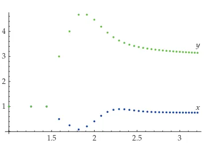
byTheorem 4.5. For the graph of 30 iterates, seeFigure 1.
Corollary 4.7. Suppose thatAi∈Crdt0,∞T,R0for alli∈1, nNandX·, s>0ons,∞Tfor
anys∈t0,∞T. Letx, y, zbe solutions of 3.1,3.2and3.3, respectively. Ify >0ont0,∞T
3 2.5
2 1.5
1 2 3 4
x y
Figure 1:The graph of 30 iterates for the solutions of4.11and4.13illustrates the result ofTheorem 4.5, hereyt> xtfor allt∈√3
3,∞√3N.
Corollary 4.8. Letxbe a solution of 3.1, andY·, s > 0ons,∞T for anys∈ t0,∞Tbe the
fundamental solution of
xΔt i∈1,nN
Aitxαit 0 fort∈t0,∞T, 4.14
andy >0ont0,∞Tbe a solution of this equation. Ifx≡yholds ont−1, t0T, thenx≥yholds on
t0,∞T.
Theorem 4.9. Suppose that there existt1 ∈ t0,∞Tand Λ ∈ Crdt1,∞T,R0such that−Λ ∈
R t1,∞T,Rand for allt∈t1,∞T
i∈1,nN
Ait≤Λt
!
1−
t
αmint
ΛηΔη
"
. 4.15
Then,3.1has an eventually positive solution.
Proof. ByCorollary 4.4, it suffices to prove that4.6has an eventually positive solution. For this purpose, byTheorem 3.1, it is enough to demonstrate thatΛsatisfies
Λt≥
i∈1,nN
Aite−Λt, αit ∀t∈t1,∞T. 4.16
Note thatΛ∈Crdt1,∞T,R0and−Λ∈ R t1,∞T,Rimply thate−Λt, sis nondecreasing
Lemma 2.6, for allt∈t1,∞T, we have
Λt≥
i∈1,nN
Ait
1−#αt
mintΛ
ηΔη ≥
i∈1,nN
Ait e−Λt, αmint
i∈1,nN
Aite−Λt, αmint≥
i∈1,nN
Aite−Λt, αit,
4.17
which implies that4.16holds. The proof is therefore completed.
Corollary 4.10. Suppose that there existM, λ∈R0 withλ1−Mλ≥1andt1∈t0,∞Tsuch that
−λi∈1,nNAi ∈ R t1,∞T,Rand
t
αmint
i∈1,nN
AiηΔη≤M ∀t∈t2,∞T, 4.18
wheret2 ∈t1,∞Tsatisfiesαmint≥t1 for allt∈t2,∞T. Then,3.1has an eventually positive
solution.
Proof. In this present case, we may letΛt:λi∈1,n
NAitfort∈t1,∞Tto obtain4.15.
Remark 4.11. Particularly, lettingλ 2 andM 1/4 inCorollary 4.10, we learn that 3.1
admits a nonoscillatory solution if−2i∈1,n
NAi ∈ R t1,∞T,Rand t
αmint
i∈1,nN
AiηΔη≤ 1
4 ∀t∈t2,∞T. 4.19
It is a well-known fact that the constant 1/4 above is the best possible for difference equations since the difference equation
Δxt axt−1 0 for t∈N, 4.20
wherea∈R , is nonoscillatory if and only ifa≤1/4see3,12.
The following example illustratesCorollary 4.10for the nonstandard time scaleTqZ.
Example 4.12. Letai ∈ R ,pi ∈ Nfori∈ 1, nNandq ∈ 1,∞. We consider the following q-difference equation
Dqxt
i∈1,nN
ai tx
$
t qpi
%
where theq-difference operatorDqis defined by3.26. For simplicity of notation, we let
which implies that the regressivity condition inCorollary 4.10holds. So that4.21 has an eventually positive solution if
Proof. As in the proof ofTheorem 4.9, we deduce that there existsΛsatisfying3.4. Hence,
ByCorollary 3.3, we havegt:yΔt i∈1,nNAityαit≤0 for allt∈t0,∞T. Then,y
ByCorollary 4.7, we know thatygiven by
yt x0Xt, t0
Proof. Solution representation formula2.3implies for a solution of4.31that
Theorem 4.15. Suppose that Ai ∈ Crdt0,∞T,R0, i ∈ 1, nN, 3.4 has a solution Λ ∈
Crdt0,∞T,R0with−Λ∈ R t0,∞T,R,xis a solution of 4.26andyis a positive solution of
the following initial value problem
yΔt i∈1,nN
Aityαit 0 fort∈t0,∞T
yt0 y0, xt ψt fort∈t−1, t0T.
4.33
Ifx0≥y0≥0andψ ≥ϕ≥0ont−1, t0T, then we havex≥yont0,∞T.
Proof. The proof is similar to that ofTheorem 4.13.
We give the following example as an application ofTheorem 4.15.
Example 4.16. LetTN3:{n3:n∈N}, and consider the following initial value problems:
xΔt 1 tx
$ 3 √
t−33
%
0 fort∈64,∞N3
xt 34−log3t fort∈1,64
N3,
4.34
where
xΔt
x$√3
t 13
% −xt
3 √
t 13−t
fort∈N3 4.35
and
yΔt 1 ty
$ 3 √
t−33
%
fort∈64,∞N3,
yt 1−2−log3t fort∈1,64
N3.
4.36
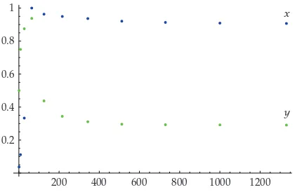
Ifxandyare the unique solutions of4.34and4.36, respectively, then we have the graph of 7 iterates, seeFigure 2, wherex > ybyTheorem 4.15.
5. Discussion
In this paper, we have extended to equations on time scales most results obtained in
1200 1000 800 600 400 200 0.2
0.4 0.6 0.8
1 x
y
Figure 2:The graph of 7 iterates for the solutions of4.34and4.36illustrates the result ofTheorem 4.15, herext> ytfor allt∈64,∞N3.
P1In2, it was demonstrated that equations with positive coefficients has slowly oscillating solutions only if it is oscillatory. The notion of slowly oscillating solutions can be easily extended to equations on time scales in such a way that it generalizes the one discussed in2.
Definition 5.1. A solution xof3.1is said to be slowly oscillating if it is oscillating and for everyt1 ∈t0,∞Tthere existt2, t3 ∈t1,∞Twitht3 > t2andαmint≥ t2for allt∈t3,∞T
such thatx >0 ont2, t3Tandxt4<0 for somet4∈t3,∞T.
Is the following proposition valid?
Proposition 5.2. Suppose that for alli∈1, nN,αi∈Crdt0,∞T,Tis a delay function andAi∈
Crdt0,∞T,R . If3.1is nonoscillatory, then the equation has no slowly oscillating solutions.
P2InSection 4, oscillation properties of equations with different coefficients, delays and initial functions were compared, as well as two solutions of equations with the same delays and initial conditions. Can any relation be deduced between nonoscillation properties of the same equation on different time scales?
P3The results of the present paper involve nonoscillation conditions for equations with positive and negative coefficients: if the relevant equation with positive coefficients only is nonoscillatory, so is the equation with coefficients of both signs. Is it possible to obtain efficient nonoscillation conditions for equations with positive and negative coefficients when the relevant equation with positive coefficients only is oscillatory?
We will only comment affirmatively on the proof of the proposition in ProblemP1. Really, let us assume the contrary that3.1 is nonoscillatory butx is a slowly oscillating solution of this equation. ByTheorem 3.1, the fundamental solutionX·, sof3.1is positive ons,∞T ⊂ t1,∞T for somet1 ∈t0,∞T. There existt2 ∈t1,∞T andt3 ∈ t2,∞Twith
αmint≥t2for allt∈t3,∞Tsuch thatx >0 ont2, t3Tandx /≥0 ont3,∞T. Therefore, we
have
for allt∈t3,∞Tand alli∈1, nN. It follows fromLemma 2.2that
xt xt3Xt, t3−
t
t3
Xt, ση
i∈1,nN
Ai
ηχt2,t3T
αi
ηxαi
ηΔη
≤ − t
t3
Xt, ση
i∈1,nN
Aiηχt2,t3T
αiηxαiηΔη
5.2
for allt ∈t3,∞T. Since the integrand is nonnegative and not identically zero by5.1, we
learn that the right-hand side of5.2is negative ont3,∞T; that is,x <0 ont3,∞T. Hence, xis nonoscillatory, which is the contradiction justifying the proposition.
Thus, under the assumptions of Proposition 5.2 existence of a slowly oscillating solution of3.1implies oscillation of all solutions.
Acknowledgment
E. Braverman was partially supported by NSERC research grant.
References
1 S. Hilger,Ein Maßkettenkalk ¨ul mit Anwendung auf Zentrumsmannigfaltigkeiten, Ph.D. thesis, Universit¨at W ¨urzburg, 1988.
2 L. Berezansky and E. Braverman, “On non-oscillation of a scalar delay differential equation,”Dynamic Systems and Applications, vol. 6, no. 4, pp. 567–580, 1997.
3 L. Berezansky and E. Braverman, “On existence of positive solutions for linear difference equations with several delays,”Advances in Dynamical Systems and Applications, vol. 1, no. 1, pp. 29–47, 2006.
4 M. Bohner and A. Peterson, Dynamic Equations on Time Scales. An Introduction with Applications, Birkh¨auser Boston, Boston, Mass, USA, 2001.
5 B. Karpuz, “Existence and uniqueness of solutions to systems of delay dynamic equations on time scales,”http://arxiv.org/abs/1001.0737v3.
6 M. Bohner, “Some oscillation criteria for first order delay dynamic equations,”Far East Journal of Applied Mathematics, vol. 18, no. 3, pp. 289–304, 2005.
7 B. G. Zhang and X. Deng, “Oscillation of delay differential equations on time scales,”Mathematical and Computer Modelling, vol. 36, no. 11–13, pp. 1307–1318, 2002.
8 I. Gy˝ori and G. Ladas, Oscillation Theory of Delay Differential Equations, Oxford Mathematical Monographs, The Clarendon Press, Oxford University Press, New York, NY, USA, 1991.
9 M. Bohner, B. Karpuz, and ¨O. ¨Ocalan, “Iterated oscillation criteria for delay dynamic equations of first order,”Advances in Difference Equations, vol. 2008, Article ID 458687, 12 pages, 2008.
10 H. A. Agwo, “On the oscillation of first order delay dynamic equations with variable coefficients,”
The Rocky Mountain Journal of Mathematics, vol. 38, no. 1, pp. 1–18, 2008.
11 Y. S¸ahiner and I. P. Stavroulakis, “Oscillations of first order delay dynamic equations,”Dynamic Systems and Applications, vol. 15, no. 3-4, pp. 645–655, 2006.