Comparison of Antenna Array Systems Using OFDM
for Software Radio via the SIBIC Model
Khoi D. Le
Department of Electrical Engineering, University of Nebraska-Lincoln, Lincoln, NE 68588, USA
School of Electrical and Computer Engineering, University of Oklahoma, Norman, OK 73019, USA Email:[email protected]
Michael W. Hoffman
Department of Electrical Engineering, University of Nebraska-Lincoln, Lincoln, NE 68588, USA Email:mhoff[email protected]
Robert D. Palmer
School of Meteorology, University of Oklahoma, Norman, OK 73019, USA Email:[email protected]
Received 31 January 2004; Revised 28 October 2004
This paper investigates the performance of two candidates for software radio WLAN, reconfigurable OFDM modulation and antenna diversity, in an indoor environment. The scenario considered is a 20 m×10 m×3 m room with two base units and one mobile unit. The two base units use omnidirectional antennas to transmit and the mobile unit uses either a single antenna with equalizer, a fixed beamformer with equalizer, or an adaptive beamformer with equalizer to receive. The modulation constellation of the data is QPSK and 16-QAM. The response of the channel at the mobile unit is simulated using a three-dimensional indoor WLAN propagation model that generates multipath components with realistic spatial and temporal correlation. An underlying assumption of the scenario is that existing antenna hardware is available and could be exploited if software processing resources are allocated. The results of the simulations indicate that schemes using more resources outperform simpler schemes in most cases. This implies that desired user performance could be used to dynamically assign software processing resources to the demands of a particular indoor WLAN channel if such resources are available.
Keywords and phrases:OFDM modulation, multipath channel, indoor radio stochastic channel model, wireless LAN.
1. INTRODUCTION
Widespread use of portable wireless systems demands max-imum efficiency in the use of fundamental resources such as frequency bands or time slots. In addition, software ra-dio applications provide the possibility for, and require the availability of, variable rates and quality of service for a large and diverse set of user needs. Extremely flexible modulation strategies such as those provided by orthogonal frequency di-vision multiplexing (OFDM) [1] mesh nicely with both the wide range of user requirements and the necessity for a soft-ware radio to be relatively easy to control via simple changes in the system programming. A potential software radio ap-plication, wireless LANs (WLANs), will be investigated using a simulation of a useful software radio modulation approach (OFDM) as well as potential software radio signal process-ing approaches that exploit antenna diversity. The utility of
antenna diversity for WLANs has been demonstrated and the development and fielding of such systems is already un-der way, see [2] for examples. The consideration of OFDM and antenna diversity as parts of a limited software radio ar-chitecture assumes that the hardware resources are already in place. At this point it is useful to focus some attention on different processing schemes and their achievable perfor-mance.
The scenario considered in these simulations is a large
20 m×10 m×3 m room, which will reasonably have two
Figure 1: Block diagram of a baseband OFDM time domain re-ceiver, adapted from [1] with addition of receiver array.
Other indoor channels listed for reference include [4,5] and those listed in [6]. It is noted here that there is a concurrent work published in [7] for modeling the impulse response in time, but this model does not feature angles of arrival.
2. ORTHOGONAL FREQUENCY-DIVISION
MULTIPLEXING SCHEME
OFDM is a modulation scheme that converts a frequency-selective channel into parallel flat fading channels by decreas-ing the symbol rate in each channel and that removes inter-symbol interference by buffering the transmitted signal. As a result, OFDM simplifies channel equalization at the receiver. OFDM remains popular, although inherent problems such as interchannel interference, phase synchronization, and high peak-to-mean power makes achieving the ideal flat chan-nel response difficult. Originally developed in the 1950s for military use, it is now found in applications such as digital terrestrial television broadcasting [8], and standards such as IEEE 802.11a and 802.11g WLAN. OFDM is also flexible in its modulation scheme, making it an ideal choice for limited software radio systems as well.
Since OFDM is an established modulation scheme, and references to it are accessible (examples include [9,10,11]), only a brief discussion of the receiver we use is provided. A block diagram of it is drawn inFigure 1.
The receiver used is a time-based receiver and has weights located directly after each antenna elements. In this config-uration, the symbols are spread over time, requiring faster processors but fewer FFT circuits. Additionally, the cyclic prefix symbols are available and can be used to estimate the channel.
3. THE STOCHASTIC IMAGE-BASED
INDOOR CHANNEL MODEL
In any receiving scheme with multiple antennas, such as a smart antenna array, the spatiotemporal correlation between the multipath components and each receiving element is of utmost importance. Simulations of receiver schemes using a channel model that produces incorrect spatiotemporal corre-lation will yield performance results that are unrealistic as the spatiotemporal correlation is a measure of the propagation scenario. For this reason, the SIBIC model (see [12,13]) is the channel model of choice. The SIBIC model is a 3D, stochastic model that combines a deterministic foundation (the image
image method is applied to find images of the transmitter, then these images are replaced with clusters whose rays have Poisson distributed arrivals, that is, exponentially distributed times-of-arrival (TOA); exponentially decaying amplitudes; and Laplacian distributed angle-of-arrival (AOA) with mean values determined by each image position. See Figure 2for visual representation of the model, andFigure 3for link be-tween the time-of-arrival, angle-of-arrival, and correspond-ing amplitude. Finally, receiver effects such as limited band-width and noninteger sampling are added to the model via filtering with a window.
Several key components of the SIBIC model will now be discussed: the partition-dependent path loss model, the sep-arable AOA distribution function, the Poisson intracluster arrival distribution function, and the intracluster ray ampli-tude function.
The partition-dependent path loss model is
PL(d)=10nlog10
4πd λc
+
W
i
Xi, (1)
wherenis the path loss exponent,dis the distance from the receiver to each virtual source,Wis the total number of walls between the receiver and the virtual source, and Xi is the
partition-dependent attenuation factor in dB.
The 3D channel impulse response is assumed separable, that is,
h(t,θ,φ)=h(t)h(θ)h(φ), (2)
whereh(t) is the TOA function,h(θ) is the zenith AOA func-tion, andh(φ) is the azimuth AOA function. This is an exten-sion of the 2D separable channel of [13].
The extended 3D angular distribution with both angles is the product of two independent Laplacian functions denoted by the expression
p(θ,φ)=√1 2σe
−|√2θ/σ|√1 2σe
−|√2φ/σ|, (3)
whereσ denotes the angular standard deviation,θ denotes the azimuth angle, andφdenotes the elevation angle. Bothθ andφare relative to their cluster mean.
X
Figure2: An overview of the proposed model. The “X” at the cen-ter of the beams represents the receiver, the solid and dashed cir-cles represent the transmitter and its images, respectively. The high-lighted room is the room of interest. The other surrounding rooms are some of the imaged rooms. The finite-width rays extending from the receiver are visualizations of the effect of introducing clusters.
Time (a.u.)
A
m
plitude
(a.u.)
(a)
Time (a.u.)
A
m
plitude
(a.u.)
(b)
Figure3: Visualization of an unfiltered impulse response for the image model and the SIBIC model. Notice that the first rays of each cluster are present in both models with the same amplitudes and time delays. However, the SIBIC model contains additional clusters, visually observed as the exponentially decreasing rays that follow the rays generated by the image model. (a) Image model. (b) Proposed model.
The equation that describes this relation is
σ2=tan−1
d1tan
σ1
d2
. (4)
In the simulations, a nominal angular spread at distancedo
Receiver
σ1 σ2
d2
d1
Transmitter Image of transmitter
Figure4: Angular spread of transmitter and its image as perceived by the receiver. The circles are visualizations of the receiver, the transmitter, and the image of the transmitter. Using basic geome-try, the width of the angular spread is calculated using a spread and a distance reference value. In this cased1andσ1are the referenced
values,d2is a known value, andσ2is the resulted calculated value.
and each distancedis used to calculate the angular spread of each cluster.
As discussed, a Poisson process describes the arrivals of the rays within each cluster, withλdenoting the intracluster (rays within the cluster) rate, Tl the arrival time of thelth
cluster, andβ(Tl) the amplitude of thelth cluster of the
Pois-son process. FromTl,dcan be calculated, and thenβ(Tl) via
(1). The time of arrivaltk+1 of the (k+ 1)st ray after thekth ray in any cluster is expressed by the conditional probability density function
ptk+1|tk
=λe−λ(tk+1−tk). (5)
The amplitude of the (k+ 1)st ray in the cluster is expressed as
βTl,k+ 1
=βTl
e−(tk+1−Tl)/γ, (6)
whereγis the exponential power delay constant of the clus-ter.
Simulation and measurement results of the channel are generally compared by examining parameters such as mean excess delay ( ¯τ), rms delay spread (στ), or power delay profile
shapes (PDP(τi)). These parameters are measures of the
mul-tipath channel response. The mean excess delay is defined as the first moment of the power delay profile relative to a power threshold (whenτ =0). The expression for the mean excess delay of a sampled PDP is
¯ τ=
τiPDP
τi
τi
τiPDP
τi
Receiver antenna Omni and microstrip Transmitter antenna Omni Receiver position (m) (x,y,z) (varies,varies,1) Transmitter position (m) (x,y,z) (5, 5, 2.9) and (15, 5, 2.9) Maximum number of reflections 3
Maximum time response (ns) 200 Exponential parameter (γ) (ns) 9.0 Poisson parameter (1/λ) (ns) 5.0 Angular spread of at 5.0 m 20.0◦
Receiver bandwidth (MHz) 100 Sampling frequency (GHz) 1.0 Hanning window time width (ns) 20.0 Path loss exponent (n) 2 Partition loss factor (X) (dB) 5
whereτidenotes the sampling time of the power delay
pro-file. The rms delay spread is the square root of the second moment of the power delay profile. The expression for the rms delay spread is
στ=
τ2−( ¯τ)2, (8)
where
τ2= τiPDP τi τ2 i τiPDP τi . (9)
Variations between simulated and theoretical values of the mean excess delay and rms delay spread exist because of the power threshold. In simulating the channel response, a threshold time is used rather than a threshold power to sig-nify when τ = 0. The threshold time is set to the first in-coming ray and is known. The parameters for simulating the channel are listed in Table 1. Also listed in this table is the SNR parameter that will be used later in the OFDM simula-tions.
Figures5 and6 are plots of the simulated mean excess
delay and delay spread for the 20×10×3 room. An
om-nidirectional and a microstrip antenna were used in simu-lating the values in each figure. The results indicate that the mean excess delay is largest near the transmitters and small-est away from transmitters. On the other hand, the trend is reversed with the delay spread. Additionally, symmetry oc-curred in both of these simulated values around the trans-mitters. According to [2], the expected values of the mean excess delay and delay spread are in the nanosecond range for an indoor environment. It is noted here that to compare simulated to measured values is difficult as the instrument, threshold level, and propagating environment are almost al-ways unique to each scenario.
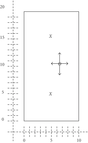
OFDM modulation is either QPSK or 16-QAM. In addi-tion, the performance of QPSK with receivers having re-alistic beam patterns is also estimated via simulations. Re-ceiver performance in small cells is important because access to base units from WLAN portable systems are from users who are generally indoor and stationary [2]. In the simulated 20 m×10 m×3 m room, two base units are placed near the ceiling and separated 10 m apart to provide good coverage. The basic setup is drawn inFigure 7, and the important sim-ulation parameters are listed inTable 1.
At the transmitter, a 32-subcarrier FFT and a chan-nel spacing of 3.125 MHz for a total receiver bandwidth of 100 MHz are used. After the FFT, a 10-sample cyclic prefix is added for a total extended time OFDM symbol sequence that is 42 samples long. The baseband sampling rate is 1 GHz. Ad-ditionally, a raised cosine window with a rollofffactor of 0.2 is used. The SNR is defined as bit energy over noise energy (Eb/N0).
The receiving scheme of a single antenna is apparent and will not be discussed. With a fixed beamformer, the angle-of-arrival of the line-of-sight (LOS) ray is assumed known, so a beam at that angle is formed. A beam is formed with
an adaptive beamformer using the optimal Wiener coeffi
-cients calculated from 50 OFDM symbols. Discussion of the adaptive scheme can be found in [14]. In both array meth-ods, the spacing between antenna elements is half the car-rier wavelength, that is,d=0.5λc. In each receiving scheme,
a 1-tap filter adapted at a step size of 0.005 based on the mean-squared criterion is used for equalization at every 6th subcarrier. The equalization coefficient of other subcarriers is achieved using linear interpolation of the in-phase and quadrature components.
The average mean-squared error (MSE) is used as a per-formance measure for each receiving scheme. It is calcu-lated by averaging the MSE of the detected and transmit-ted frequency symbols across 32 subcarriers and over 500 symbols at each position within the room. At each position, 1000 OFDM symbols (1050 for the adaptive beamformer) are transmitted. With the single-element receiver and fixed beamformer, the first 500 symbols are for adapting the equal-izer and the last 500 symbols are for calculating the MSE. With the adaptive beamformer, 50 additional symbols are transmitted beforehand for estimating the Wiener filter co-efficients. It is noted here that 500 symbols for adapting the equalizer is a generous value, but it allows for a small step size and assured stability of the equalizer to reach a steady-state MSE at most positions within the room.
(a) (b)
0 5 10 15 20
Mean excess delay (ns)
Figure5: Simulated mean excess delay of channel using parameters inTable 1. (a) Omnidirectional. (b) w/ beam pattern.
the narrowband assumption is safe. The channel is normal-ized at one antenna element so that the SNR can be easily defined for the simulations. Additionally, the same channel is used in each receiving scheme in all following subsections and the channel is assumed time constant at each position.
4.1. QPSK
The MSE of the three receiving schemes with QPSK modu-lation and omnidirectional antennas are plotted inFigure 8. Recall the base units are located at (5, 5, 2.9) and (15, 5, 2.9). Visually, the single-element receiver has the poorest per-formance, the fixed beamformer is better, and the adaptive beamformer is best. There is an observable difference of at least 5 dB centered around the positions of both base units, with the best performance achieved using the adaptive beam-former. For an arbitrary MSE value of −10 dB, the fraction of positions with MSE below this value is 1, 47, and 99 per-cent for the single element, fixed beamformer, and adaptive beamformer, respectively.
Since the single element receiver has equal gain toward all angles, the fixed beamformer has highest gain in the LOS angle, and the adaptive beamformer uses the approximate Wiener solution, the improvement trend from single ele-ment to adaptive beamformer is reasonable. Moreover, it is expected that the SNR of the fixed beamformer in the LOS angle increases by the number of antenna elements. For the adaptive beamformer, analysis of the resultant beam pattern (not plotted) shows that the mainlobe in the simulations
(a) (b)
0 5 10 15 20
Delay spread (ns)
Figure6: Simulated delay spread of channel using parameters in
Table 1. (a) Omnidirectional. (b) w/ beam pattern.
20
15
10
5
0
0 5 10
X
X O
Figure7: General simulation scenario. The two “X’s” represent the two base units. The “O” represents the mobile unit, which is posi-tioned at various locations in the room. The dimension of the room is 20×10×3 m3. The base units are located at a height of 2.9 m. The
(a) (b) (c)
−25 −20 −15 −10 −5 0 5
MSE (dB)
Figure8: Average MSE of 32 subcarriers, averaged over 500 OFDM symbols, with 4-QAM modulation. (a) 1 element M=6. (b) Fixed beamformer M=6. (c) Adaptive beamformer M=6.
was directed at the LOS ray and nulls were place towards strong multipath rays. This angular response pattern is sen-sible since multipath signals distort the signal from the LOS ray, which is the signal of interest. In addition, the lowest MSE values are obtained near the base units where the spread of the channel is at a minimum. It is also noted here that since the wavelength at 60 GHz is only 5 mm, the channel is signifi-cantly different between sampled positions. This is a possible reason why high and low MSE squares are occasionally next to each other.
4.2. 16-QAM
With omnidirectional antennas, the MSE of the three receiv-ing schemes are simulated again, but this time with 16-QAM. The results are plotted inFigure 9. As was noted, the SNR is kept constant by reducing the noise power by√2 from QPSK to maintain the same bit-energy-to-noise-power ratio. The improvement in MSE from 4-QAM to 16-QAM is 0.2, 0.2, and 1.2 dB for single element, fixed beamformer, and adap-tive beamformer, respecadap-tively. It is noted here that this im-provement in MSE does not directly correspond to better performance since signal constellations with different den-sities are being compared.
4.3. QPSK with beam pattern
In an outdoor environment, the base and mobile units are widely separated. As a result, modeling the receiving
antennas as omnidirectional is justified since the multipath signals are mostly from angles near the horizon and the an-gular response for a vertical dipole is uniform in azimuth. However, the mobile and base units in an indoor environ-ment are near each other and the elevation angle can no longer be assumed to be from near the horizon. Therefore, the system performance is dramatically affected by the angu-lar response of the antennas, particuangu-larly at the null angles of the antennas. It is beneficial then to simulate the angular response for a realistic pattern rather than with an assumed omnidirectional pattern to investigate the performance of a receiver that is located indoor.
In this subsection, the receiver performance with QPSK modulation is simulated using antenna elements having an-gular responses modeled after a realistic microstrip antenna pattern measured in [15]. The duplicated pattern is plotted inFigure 10. Differences between the duplicated and original pattern are twofold. First, the gain of the duplicated pattern is several dB higher at elevation angles greater than 60 degrees from vertical. Second, the duplicated pattern is normalized to the gain at the vertical angle, whereas the original pattern is not normalized.
(a) (b) (c)
−25 −20 −15 −10 −5 0 5
MSE (dB)
Figure9: Average MSE of 32 subcarriers, averaged over 500 OFDM symbols, with 16-QAM modulation. (a) 1 element M=6. (b) Fixed beamformer M=6. (c) Adaptive beamformer M=6.
90
60
30
0
330
300 270
240 210
180 150
120
−20
−10 0 10
Figure10: Radiation pattern response for microstrip antennas at 60 GHz, adapted from [15] with a sinc function of order 2.
the number of positions with better performance is 81, 73, and 68 percent. Overall, this means that simpler receiving
schemes improve more compared to sophisticated receiv-ing schemes with directive antennas. In addition, it is no-ticed that most improvement occurs at positions where the angles of the mobile unit may be in the center of either the main or sidelobes of the antenna beam pat-tern, and most degradation occurs at positions where the mobile units are at the nulls of the antenna beam pat-tern.
5. CONCLUSION
(a) (b) (c)
−25 −20 −15 −10 −5 0 5
MSE (dB)
Figure11: Average MSE of 32 subcarriers, averaged over 500 OFDM symbols, with 4-QAM modulation. A microstrip antenna pattern was applied, as compared to previous simulation cases using omnidirectional antennas. The small (5 pixels wide) circle corresponds to the base unit being at 60 degrees, while the large (13 pixels wide) circle corresponds to the base unit being at 30 degrees, in elevation with respect to the mobile unit. (a) 1 element M=6. (b) Fixed beamformer M=6. (c) Adaptive beamformer M=6.
REFERENCES
[1] T. Keller and L. Hanzo, “Adaptive multicarrier modulation: a convenient framework for time-frequency processing in wire-less communications,”Proc. IEEE, vol. 88, no. 5, pp. 611–640, 2000.
[2] T. S. Rappaport, A. Annamalai, R. M. Buehrer, and W. H. Tranter, “Wireless communications: past events and a future perspective,”IEEE Commun. Mag., vol. 40, no. 5, pp. 148–161, 2002.
[3] K. D. Le, M. W. Hoffman, and R. D. Palmer, “Three-dimensional propagation model for wireless LAN distribution of software radio,” inProc. IEE Colloquium on DSP Enabled Radio, Livingston, Scotland, UK, September 2003.
[4] R. Heddergott and P. E. Leuthold, “An extension of stochas-tic radio channel modeling considering propagation environ-ments with clustered multipath components,”IEEE Trans. An-tennas Propagat., vol. 51, no. 8, pp. 1729–1739, 2003. [5] C.-C. Chong, C.-M. Tan, D. I. Laurenson, S. McLaughlin, M.
A. Beach, and A. R. Nix, “A new statistical wideband spatio-temporal channel model for 5-GHz band WLAN systems,”
IEEE J. Select. Areas Commun., vol. 21, no. 2, pp. 139–150, 2003.
[6] R. B. Ertel, P. Cardieri, K. W. Sowerby, T. S. Rappaport, and J. H. Reed, “Overview of spatial channel models for antenna array communication systems,”IEEE Pers. Commun., vol. 5, no. 1, pp. 10–22, 1998.
[7] J. Kunisch and J. Pamp, “An ultra-wideband space-variant
multipath indoor radio channel model,” inProc. IEEE Con-ference on Ultra Wideband Systems and Technologies (UWBST ’03), vol. 1, pp. 290–294, Reston, Va, USA, November 2003. [8] H. Sari, G. Karam, and I. Jeanclaude, “Transmission
tech-niques for digital terrestrial TV broadcasting,”IEEE Commun. Mag., vol. 33, no. 2, pp. 100–109, 1995.
[9] R. Van Nee and R. Prasad, OFDM for Wireless Multimedia Communications, Artech House, Boston, Mass, USA, 2000. [10] L. Hanzo, M. M¨unster, B. J. Choi, and T. Keller, OFDM
and MC-CDMA for Broadband Multi-User Communications, WLANs and Broadcasting, John Wiley & Sons, Chinchester, UK, 2003.
[11] J. Heiskala and J. Terry,OFDM Wireless LANs: A Theoretical and Practical Guide, SAMS, Indiana, USA, 2002.
[12] K. D. Le, M. W. Hoffman, and R. D. Palmer, “A stochastic image-based indoor channel model for use in ultra-wideband 3-D sensor array simulations,” inProc. IEEE Conference on Ul-tra Wideband Systems and Technologies (UWBST ’03), vol. 1, pp. 300–304, Reston, Va, USA, November 2003.
[13] Q. H. Spencer, B. D. Jeffs, M. A. Jensen, and A. L. Swindle-hurst, “Modeling the statistical time and angle of arrival char-acteristics of an indoor multipath channel,”IEEE J. Select. Ar-eas Commun., vol. 18, no. 3, pp. 347–360, 2000.
[14] B. Farhang-Boroujeny,Adaptive Filters: Theory and Applica-tions, John Wiley & Sons, Chinchester, UK, 1998.
Khoi D. Lereceived the B.S. and M.S. de-grees in electrical engineering from the Uni-versity of Nebraska at Lincoln in 1999 and 2001, respectively. Currently, he is working towards the Ph.D. degree at the University of Oklahoma, where he is conducting re-search in the signal processing of remotely sensed data of atmospheric scatterers with radars. His interests include wireless com-munications, adaptive filtering techniques, and stratiform clouds.
Michael W. Hoffmanreceived the B.S. de-gree from Rice University, Houston, Texas, the M.S. degree from the University of Southern California, Los Angeles, and the Ph.D. degree from the University of Min-nesota, all in electrical engineering. From 1985 to 1988, he was a signal processing sys-tem engineer in the Space Communications Division of TRW Inc. In 1993, he joined the University of Nebraska-Lincoln, where
he currently serves as an Associate Professor. His research interests include data compression, joint source-channel coding, and sensor array processing.
Robert D. Palmerreceived his Ph.D. degree in electrical engineering from the University of Oklahoma, Norman, Oklahoma, in 1989. His Ph.D. studies focused on the applica-tions of advanced signal processing tech-niques to atmospheric radar. From 1989 to 1991, he was a Postdoctoral Fellow at the Radio Atmospheric Science Center, Kyoto University, Japan. After his stay in Japan, Professor Palmer held the position of a