A method for the interpretation of three dimensional equatorial GDV fields

141 Copy right © The Society of Geomagnetism and Earth, Planetary and Space Sciences (SGEPSS); The Seismological Society of Japan; The Volcanological Society of Japan; The Geodetic Society of Japan; The Japanese Society for Planetary Sciences. 1. Introduction

The geomagnetic variations (GV) are due to the iono-spheric-magnetospheric current systems, and to the currents induced by them inside the Earth. So, they have been extensively used to infer external current morphology and Earth’s structures.

When the geometry of the source must be taken into account, as is the case for example for storm-time and geomagnetic daily variations (GDV) fields, the first step that must be achieved to analyze GV fields, is to separate them into parts of internal and external origin.

Once this task is performed, some characteristics of the external current system and its variations with solar terrestrial conditions may be inferred from the external field. Also the Earth’s structure may be investigated, by predicting the field induced by the external field in a model of the suspected structure and comparing it with the internal field.

In the case of the GDV fields the frequencies involved are low enough to allow to the signal to penetrate down to upper mantle depths and, so, by using these variations the structure of this Earth’s layer may be inferred (see e.g. Campbell, 1987).

In particular, at equatorial latitudes, the GDV were assumed to be bi-dimensional, and then, they were separated by performing the Kertz operator of the field components, as proposed by Kertz (1954). To perform this transform the involved function must be specified in a profile ranging from –∞ to ∞, which is a priori impossible in the case of the application to equatorial GDV fields, since they are measured within a finite interval.

The field components are enhanced in a small latitude interval around the equator. Based on this fact, the first

attempt to solve the above problem was to represent the total field as a sum of two parts: an incremental or “electrojet” and an extended or planetary parts, respectively. In such a way that the electrojet part is made zero out of a finite interval around the dip by a suitable choice of the extended part. The Kertz operator was then applied only to the incremental part. To separate the planetary part the values of the ratio of the internal to the external contribution were assumed to be equal to 0.4 and –0.4 for the horizontal and the vertical components, respectively. These values correspond to the global average of the ratio of the first few terms of the spherical harmonics analysis of the Sq field (see e.g. Forbush and Casaverde, 1961; Onwumechilli, 1967; Fambitakoye and Mayaud, 1976). This procedure implies the assumption that the Earth’s layers are laterally homogeneous and that the conductosphere begins everywhere at its average depth which is approximately 650 km (see e.g. Osella and Duhau, 1983).

Nevertheless, by comparing rocket measurements of geomagnetic field variations at E-region heights with GDV data, the presence of a strong inhomogeneity in the conductosphere layer has became apparent (Duhau and Romanelli, 1979; Duhau et al., 1982).

Therefore, in order to make the method applicable to the above case a different approach has been introduced by Duhau and Osella (1982): a suitable continuation of the field at the end of the measured profile was provided and then the Kertz operator was applied to the total field. In that way it was found that the conductosphere’s depth varies strongly around the Earth, and seems to be related to tectonic features. It was found, also, that the equatorial dip may be running along deep discontinuities in the Earth’s conductivity (see Duhau and Favetto, 1990 and references therein).

The external GDV field is approximately bi-dimensional only around noon and near the equator, and will induces a field with the same geometry only in the case that the local

A method for the interpretation of three-dimensional equatorial GDV fields

Silvia Duhau and Ernesto A. Martínez

Laboratorio de Geofisica, Departamento de Fisica, Universidad de Buenos Aires, Ciudad Universitaria Pabellón I, (1428) Buenos Aires, Argentina

(Received February 17, 1997; Revised December 9, 1997; Accepted December 17, 1997)

142 S. DUHAU AND E. A. MARTÍNEZ: INTERPRETATION OF THREE-DIMENSIONAL EQUATORIAL GDV FIELDS

Earth’s structure does not have discontinuities running along the direction normal to that of the electrojet current vector. So, to assume that the field is bi-dimensional severely limits the applications of the above methods. Moreover, even in the bi-dimensional case, it will be convenient to evaluate the important of the East West derivative due to the variation on local time.

To be able to make this evaluation and to separate GV at times, latitudes or frequencies other than local noon at the equator and at daily frequencies, a method to separate three-dimensional GV fields is needed. In particular this will allow the use of the equatorial GDV data to investigate the structure of the upper mantle in the general case.

In the present paper, to analyze GDV fields, we apply a system equation developed by Hartmann (1963) and by Weaver (1963), that allows separating any three-dimensional low frequency field known over a plane surface into parts originated above and below the surface. This system equation is based on the Riesz transform that includes singular inte-grals. So to apply it we introduce a mathematical algorithm able to compute the principal values of a singular integral. After the field is separated, a theory must be introduced to interpret the results. For the bi-dimensional case the external field was interpreted by assuming very simple forms for the external field (see e.g. Onwumechilli, 1967; Duhau and Favetto, 1990). In the present paper we introduce a theory based on the Fourier transform that allows to represent general three-dimensional fields together with a general formulae to infer, from the external field so described, the field induced in an horizontally layered Earth’s model.

Most of the GDV equatorial data have been measured in North-South chains. Therefore, to increase the information that may be obtained from these data, we discuss the ap-plication to them of the above separation method and in-terpretation theory. This is possible under a hypothesis that the East-West coordinate is equivalent to the time coordi-nate in the reference frame fixed to the sun (Campbell, 1987).

As an example we apply the method to GDV data from India (Indian Institute of Geomagnetism, 1983), and the results are commented in Section 4.

2. The Method of Separation of GV Fields into Part of Internal and External Origin

2.1 Theory

We restrict ourselves to low frequencies, such that the displacement current is negligible, and we assume that there are no sources at ground. Thus, the magnetic field, Br, is given by:

Br= −∇Ω,

( )

where Ω is the scalar potential that satisfies, both, the Laplace equation:

∇2 =

( )

0 2

Ω ,

and the boundary conditions.

We assume a plane geometry, and therefore the Fourier transform may be applied to solve Eq. (2). The general solution found by this procedure is (see e.g. Weaver, 1963):

Ω Ω= e+Ωi.

( )

The coordinate system, (x,y,z), is defined as usual: north-ward, eastnorth-ward, and downward respectively. In that coor-dinate system, the subscripts e and i refer to the potentials originated in sources that are in the z < 0 (external) and in the

z > 0 semi space, respectively, and:

forms of the vertical component of the field of external and internal origin, respectively.

The application of the Riesz transform to the separa-tion of a potential field A system equation that allows separating any potential field known over a plane into parts originated by sources located above and below the plane may be found by using the formalism of the previous section. The procedure may be summarized as follows (Hartmann, 1963; Weaver, 1963): introducing Eqs. (3) and (4) in Eq. (1) and applying the convolution theorem, it is found that the internal and external parts of the GDV field component (X,Y,Z), are given by:

Xe,i=1 2/

[

]

( )

Ye,i =1 2/

[

]

( )

Ze,i =1 2/

[

]

( )

respectively. In the above equations Rif are the Riesz transforms of the function f, defined as:

N₂

In the case that the field is two-dimensional, and the coordinate system is selected such that f depends only on x,

R1 reduces to the Kertz operator and R2f and Y are indentically

zero.

Equations (5) and (6) allow to separate the components of a three-dimensional field, which are known over the plane z

= 0, into parts of internal (z > 0) and external (z < 0) origin. However, since N1,2→ ∞ for u, v →x,y, performing the Riesz

transforms implies to compute integrals of singular functions. Therefore to apply the above equations this problem should be solved first. In the following we discuss a method that allows computing the principal value of Eq. (6).

2.2 A numerical method to compute the Riesz transform

The Riesz transforms are singular integrals. Therefore the ordinary methods of numerical integration like Simpson, variable quadrature or Monte Carlo are not suitable to compute them. To solve this problem the field may be represented in a basis L2_{() whose Riesz transforms are}

analytical functions, as for example the Fourier one, and then the Riesz operator applied over the components of that basis. In fact, Agarwal and Weaver (1990) used this procedure to compute the Kertz operator.

From the convolution theorem Eq. (6) may be rewritten as: regular function is also a regular function and that C1,2→ ±i

for ξ, η → ±0 so the arguments of the inverse Fourier transforms in Eq. (7) does not have singular points and then the involved integrals may be computed by the standard numerical algorithms. To perform the Fourier transforms (and inverse transforms) we have used the Fast Fourier transform algorithm as given by Press et al. (1992).

To test the numerical method we have applied it to a dipole field. As for any potential field, the components of the dipole field are related by the Riesz transforms as (see e.g. Weaver, 1963):

b_x=R₁b_z,

( )

b_y=R₂b_z.

( )

The numerical computations of the Riesz transforms necessitate an evaluation of the integrals involved in Eq. (7) over a finite domain instead of over the entire real plane. To evaluate the error introduced by this limitation we have computed the Riesz transforms of bz, from its analytical expression, over an square domain of side nh with n an in-teger and h the height above ground at which the dipole is located. Thus we have compared the values of bx and by obtained from Eq. (8) by this procedure, with the values obtained from the corresponding analytical expressions. For thex component we found that for n > 3 the relative error is less than 0.2% in the center of the square, increasing to the border of the square and minimizes at n = 5 in which case is of around 5% at the border. The results are similar for the y

component.

2.3 Some comments about the application to low fre-quencies GV fields

Equations (5) and (6), these last computed with the nu-merical algorithm discussed in Subsection 2.2, may be applied to a field known over a plane surface at a fixed time, to separate the field into the part originated by sources above the plane from that originated below.

The assumptions involved in the derivation of Eqs. (5) and (6) are that the displacement current may be neglected and there are no sources of the field at ground. The first ap-proximation sustains only for low frequency fields and the second, due to the low conductivity of the Earth at ground, for any frequency. None of the above assumptions implies a restriction on the geometry of the source and so both, the UT and the LT, time variations of the signal are taken into account if the method is applied to GV measured over a region at a fixed UT (see also Takeda, 1991).

The method implies plane geometry, in the case of the GDV fields the domain over which the field is measured is a spherical surface. We have evaluated the error introduced by approximating it by a plane surface. We found that this is less than 0.1%.

Instead of a discrete Fourier spectrum of the GDV, like in the spherical harmonic analysis of these variations, to use the Fourier transform formalism allow describing continuum spectrum. This feature makes the method specially suited for the application to equatorial data since—as was discussed by Chapman and Bartels (1940)—a discrete spectrum do not allows to describe the sharp equatorial enhancement of the GDV field accurately enough.

The inference of ionospheric currents at daylight times from the external field In analyzing the Global GDV field by the spherical harmonic expansion of its components, it is usually assumed that the currents are circulating in an infinitesimal layer concentric with the earth (see e.g. Chapman and Bartels, 1940). Similarly we may assume that the ionospheric current is circulating in an infinitesimal layer located a constant height h (=107 km).

144 S. DUHAU AND E. A. MARTÍNEZ: INTERPRETATION OF THREE-DIMENSIONAL EQUATORIAL GDV FIELDS

where zˆ is a unit vector in the vertical direction.

3. A Method to Analyses GDV Field Measured in North-South Profiles

The interest in the equatorial electrojet phenomenon has lead to many researches to measure the GDV field around the equator. The electrojet flows along the dip equator and, around noon, its East-West extend is very large as compared with its North-South one. Therefore most of the measure-ments have been performed along magnetometer chains aligned, as far as possible, to a meridian. Then, the data so obtained have been interpreted by assuming that the electrojet is bi-dimensional in a Cartesian coordinate system with one of its axis aligned with the dip equator (see e.g. Onwumechilli, 1967; Duhau and Favetto, 1990).

Notices that due to the bi-dimensional geometry assumed by the above methods only local noontime values of south-north profiles of the GDV components may be considered. This implies that, both, UT and LT are lost when applying them.

However, the LT variation of these profiles may be used to infer three-dimensional fields by making the assumption that the GDV are stationary in a coordinate system fixed to the Sun (Campbell, 1987) and, therefore, taking the temporal variation as equivalent to the East-West one. In fact, this approximation which leads to lost UT variations is made when applying spherical harmonic expansion to analyze Sq

fields (see e.g. Chapman and Bartels, 1951; Matsushita, 1967; hereafter, M67).

3.1 Theory

The external field We assume that the ionospheric current system that leads to the field is stationary in the coordinate system fixed to the sun. Therefore, in that co-ordinate system the scalar potential field from which the external magnetic field, Br_e, may be derived (Eq. (4)) is stationary.

To find the expression of the field as seen in the coordinate system moving with the Earth we should perform a Lorentz transformation.

For non-relativistic velocities the convective electrical currents may be neglected (Takeda, 1991) and so the mag-netic field is invariant. Then the potential function, Ωeg, from

which that field may be derived in the Earth’s frame is given by:

Ωe Ω

g e

=

(

)

( )

whereu is the tangential component of the earth rotation velocity at the earth’s surface.

It is readily shown that the solution of Eq. (2) for a potential function of the form (10) is given by Eq. (4) with definition (4.1), and definition (4.2) replaced by

∏ =e

[

(

(

)

)

]

(

)

On the other hand, when UT variations are ignored the external electric field is stationary in the Sun’s reference frame. Therefore the induced current are made not by the time variation of this field but by the time derivative of the dynamo field, Er_e, as seen in the frame fixed to the Earth, which is given by (see e.g. Takeda, 1991):

Ere= − ×u Br re,

( )

where for simplicity we have omitted the superscript g. From this and Eqs. (1) and (4) (with definitions (4.1) and (10.1)), it follows: derivative of the external field as seen in the Earth’s refer-ence frame are related by:

The field induced within the Earth The external electric field induces in the Earth currents whose characteristics depend on the boundary conditions imposed by the Earth’s structure, therefore it is impossible to predict the field induced by the external field in general case. Nevertheless, the solution of this problem for the case of a horizontally stratified Earth model may be found by the Fourier transform formalism, and is presented in the next paragraph.

The field induced on a horizontally stratified Earth model The potential function of the magnetic field induced in the Earth’s interior by a field whose potential is of the form (10) is given by:

Ωi Ω

g i

=

(

)

( )

As in the previous paragraph, the solution of Eq. (2) for a potential function of the form (14) is given by Eq. (4) with definition (4.1) and definition (4.2) replaced by:

∏ =i i

[

(

(

)

)

]

(

)

Similarly, the induced field inside the conductor is found to be of the form: andβk may be found by applying the boundary conditions at each interface and θk are constants that are determined by imposing the restriction that the diffusion equation (see e.g. Price, 1950):

must be fulfilled within each conducting layer: In the above equationσk is the conductivity of the layer k. Introducing (14) on that equation, it follows that:

θk ξ η π ησu k

2 2 2

4 16 2

= + − i .

(

)

The magnetic field inside the conductor is found by introducing (16) in the Faraday’s law and taking into account (10). Finally the solution is obtained by introducing the boundary conditions for the magnetic field at each interface. Price (1950) found the solution for a semi-infinite con-ductor and a field of the form (16.1) with P an arbitrary function. It is easy to generalize it to a layered model (see also Duhau and Favetto, 1990) and to apply it to a field of the form (14), we find:

withα1 given by the recurrence formulae:

α θ θ α θ θ

Once the GDV are separated into parts of internal and external origin—by applying Eqs. (5) and (6)—Equations (17) and (18) allow to predict the field induced by the external field on a horizontally stratified Earth.

3.2 Application

The method of interpretation presented above requires that the tangential velocity at the Earth surface being a constant. The error that this approximation introduces in the determination of the phase shift between the external and the internal field is 0.1% at the equator and increases with latitude, being 5%, at the latitude of 30°.

To improve the precision when computing the Riesz transforms is convenient to make same estimation of the components beyond the measured profiles, instead to make the field zero there (as in the example of Subsection 2.2). For GDV equatorial data the best approximation is to use the Global field as described by the spherical harmonic analysis of Global data obtained at the same solar activity, and normalizes it to the value of the measured field at the border of the measured surface. That criterion is a generalization for three-dimensional GDV fields of the criterion proposed by Duhau and Osella (1982) for bi-dimensional GDV fields.

3.3 Some comments about the inference of the upper mantle structure

To apply equatorial GDV North-South profiles to the inference of upper mantle structures, the noon amplitudes of the components of the GDV field were separated by the Kertz operator. The external part of the field thus separated was assumed to be a single diurnal wave, which was rep-resented by the sum of an incremental and an extended part. This last was represented by a sum of a constant and a single harmonic function—withη = 0 and ξ = 7.6 × 10–7 _m–1_—.

146 S. DUHAU AND E. A. MARTÍNEZ: INTERPRETATION OF THREE-DIMENSIONAL EQUATORIAL GDV FIELDS

conductosphere depth near dip equator was found (see e.g. Duhau and Favetto, 1990, and references therein).

The method presented here allows finding the wave spec-trum of the internal and external GDV fields, and so it may be applied to solve more realistic Earth’s models. In particu-lar, the two-dimensional method allows to find the ratio of the amplitudes A (=|α|) but not the phase shift φ (=arctan(imag(α)/real(α))) between the internal and exter-nal fields, and therefore even in the simplest case of a single harmonic wave the three-dimensional method improves the information that may be found from equatorial GDV fields. To illustrate this point, we have computed the parameter

α—from Eq. (18) with θk given by Eq. (16.2)—for single diurnal (η = 1.6 × 10–7 _m–1_{) and semidiurnal (}η _{= 3.2} × ₁₀– 7 _m–1_{) waves with} ξ _{= 7.6} × ₁₀–7 _m–1_{, and for a three-layered}

Earth’s model: a non conducting layer followed by a 0.1 mho/m layer of thickness Δp above a semi infinite perfect conductor with a plane boundary located at a depth pc. This

Fig. 1. The ratio of the internal to the external parts of the noon amplitude of the diurnal geomagnetic variation and the phase shift of the internal with respect to the external field for the diurnal and semidiurnal geomagnetic variations. For the case of a three layered conductivity model: a not-conducting layer followed by a 0.1 mho/m layer of thickensΔp above a semi-infinite perfect conductor with its boundary at a depth pc.

Fig. 2. The location of the Indian geomagnetic observatories and the tectonic features that delimit the Indian Plate (this last has been adapted from The National Geographic Magazine, 1995).

simple model was selected since, according to the result of Duhau and Favetto (1990), the layers that contributes appre-ciably to GDV fields are the conductosphere and a less conductive layer above it. Also, the conductosphere con-ductivity may be considered infinite at daily frequencies, and that of the less conducting upper layer has been well determined from magnetotelluric methods (see e.g. Riesz, 1983).

Figure 1 shows the ratio for the diurnal variation—which for the semidiurnal is almost the same—and the phase shift for the diurnal and semidiurnal variations. Note that for a given value of A there is an infinite set of values of pc and Δp

and, so, only a minimum value of pc may be determined,

which corresponds to the case Δp≡ 0 (see also Duhau and Favetto, 1990).

However,φ depends on Δp, which allows determining univocally the actual set. For example, for the average global case pc = 600 km and Δp = 200 km (see e.g. Pecovä

et al., 1987) A≅ 0.4 and φ ≅ 20 min (5°) for the diurnal and

φ ≅ 60 min (15°) for the semidiurnal variations, respectively. These values are in the range found by the spherical harmonic analysis of global data (see e.g. M67, and references therein). Local values of the conductosphere depth ranging from 250 km to 1000 km where obtained from equatorial GDV data (Duhau and Osella, 1985 and references therein). Consequently, local values of the ratio between the internal and the external fields for the daily frequency are ranging roughly from 0.7 to 0.2 (see Δp = 0 curve in Fig. 1).

148 S. DUHAU AND E. A. MARTÍNEZ: INTERPRETATION OF THREE-DIMENSIONAL EQUATORIAL GDV FIELDS

value sustain for the planetary field, precludes the applica-tion of that methods to the study of local variaapplica-tion of the upper layer structure. Also, it may introduce distortions in the separated internal and external parts of the electrojet fields.

The above simple model was presented only as a mode of an example. To find the actual structure of the upper mantle and its conductivity distribution, the entire wave spectrum should be considered, even at noon. In particular, the layers laying above the conductosphere must be investigate with the help of higher frequencies, since these layers may contribute to the phase shifts of the GDV wave spectrum. Also, the Indian equatorial zone is surrounded by the ocean

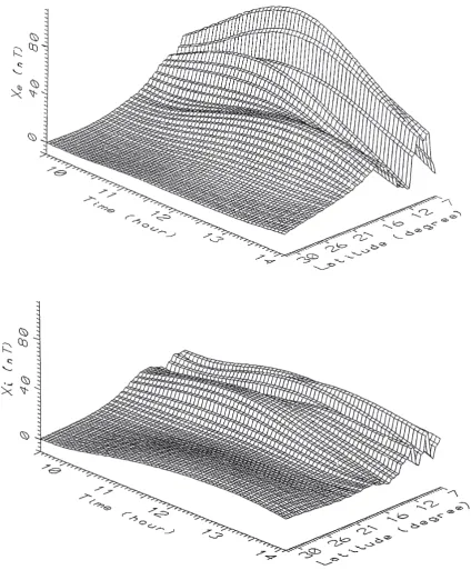
Fig. 4. The external, Xe, and the internal, Xi, parts of the northward component of the GDV field of Fig. 3 in the interval covered by the Indian observatories.

that extend from the dip equator freely to the south (see Fig. 2) and highly inhomogeneous distribution of land and ocean, may substantially contribute to the phase shifts for daily frequencies (Takeda, 1991).

3.4 Application to the Indian equatorial North-South chain

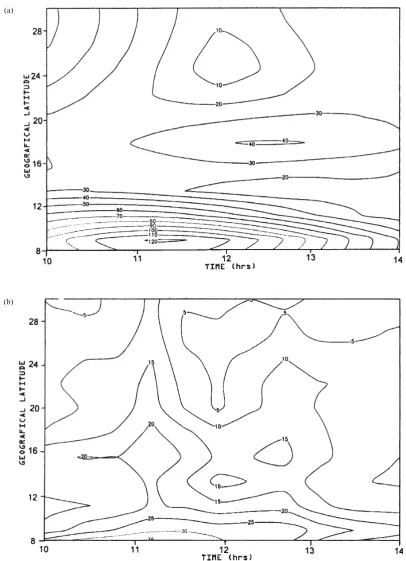
Fig. 5. Equal intensity contours of the horizontal GDV field (a) the external and (b) the internal parts, respectively (1 unit = 1 nT).

We have taken the coordinate axes as in the previous paragraph, with the x-axis along the dip equator. To com-plete the field profiles outside the North-South interval covered by the magnetometer chain, the global field repre-sented by a spherical harmonic series as given by Chapman and Bartels (1940) for the year 1905 (a year of a solar activity similar to that of the data) has been used.

It should be observed that all but one geomagnetic station (Trivandrum, dip latitude 1.03°S) are located to the north of the dip equator. So, to the north of Sabhawala (20.95°N) the

North-South profiles of the field components for each hour have been completed using the global field. It was not possible to do the same to the south since the spherical harmonic analysis does not represent properly the GDV field at electrojet latitudes (see e.g. Chapman and Bartels, 1940). Therefore, to complete the profile of the X and Z

components to the south of Trivandrum, the global field was subtracted from the total field in the measured interval of latitudes at the north, and the result was added to the global field. Finally, we have interpolated the experimental values

150 S. DUHAU AND E. A. MARTÍNEZ: INTERPRETATION OF THREE-DIMENSIONAL EQUATORIAL GDV FIELDS

by a three-degree spline algorithm, the data so processed are shown in Fig. 3.

The separation of the field We have applied Eq. (5) to the above data with the help of the algorithm presented in Subsection 2.2 (Eq. (7)). The external and the internal parts of the X component thus found around noon times are shown in Fig. 4. On that figure we have restricted ourselves to the North-South interval covered by the Indian data. Out of this interval the data correspond to a global average and have been only used to evaluate the Riesz transform.

The external and the internal fields By introducing the external field in Eqs. (17) and (18) the field induced by this in a given Earth’s model may be computed. According to previous results we have assumed a two layered model, consisting in: a non conducting horizontal layer up to a deep of 1000 km, and semi infinite perfect conductor below (Ramaswamyet al., 1985; Chamalaun et al., 1987; Favetto

et al., 1992).

Figure 5 shows the equal intensity contours of the horizontal GDV field. The two-layered model predicts a field distri-bution which morphology is quite similar to the external one. While the actual internal distribution (Fig. 5(b)) is similar to the external (Fig. 5(a)) only near the equator but has striking differences beyond 12°N.

These departures of the computed horizontal field distri-bution from the actual one indicate the presence of an inhomogeneous conductivity distribution in the region. Evidence for a strong inhomogeneity at the North-west of India, was found also by Parkinson (1987) in data from Aroraet al. (1982).

This results may be interpreted by observing the highly inhomogeneous distribution of land and ocean and the strong tectonic features that has the Indian region (see Fig. 2).

In fact, model computations of the induction effect of the GDV in a realistic model of ocean-land distribution indicate that two strong current vortices are produced by these variations in the ocean around the Indian region (see figure 2 in Beamish et al., 1983 paper). This system current may substantially contribute to the total GDV at land in that region.

Also, according to previous results (see e.g. Duhau and Osella, 1985, and references therein), some tectonic features are associate to lateral discontinuities in the Earth’s struc-ture at upper mantle depths that leads to lateral conductivity contrasts.

In particular, in India the contact between the Eurasian and the Indian plates might be associate to a large conduc-tivity contrasts. This tectonic feature is just near the Sabhawala observatory, which is located too far—more than 12,000 km—from the next observatory (Alibag) (see Fig. 2). This lack of data may leads to a large error in the interpolated field components, more since these might be very irregular there. Therefore, a denser chain of observa-tories is needed around the contact between the plates in order to have the necessary data to make a quantitative study of this interesting tectonic feature.

4. Summary and Conclusions

We have developed a method of interpretation of

three-dimensional GDV fields at equatorial latitudes based on the Riesz and the Fourier transforms formalism.

The method has two steps:

(1) The field components are separated in external and internal parts by the application of the Riesz transform trough the system equations obtained by Weaver (1963) and by Hartmann (1963) (Eq. (5)). The Riesz transforms are singular integrals; therefore an algorithm based on the Fourier transform is introduced to find the principal value of a singular integral (Eq. (7)). By applying the fast Fourier transform to the numerical code that build up this algorithm the separation of the field components is performed in real time.

(2) The external current system is found from the Fourier transform of the downward component of the external field (Eq. (9)). And the field induced by the external field in horizontally layered model is computed from Eqs. (15) and (16). By comparing the field so computed with the actual one, the parameters of the conducting layers may be found in the case that the upper mantle layers underneath are laterally homogeneous. Otherwise the upper mantle lateral inhomogeneity are detected, and by comparing it with the tectonic features of the region, a realistic laterally inhomogeneous model may be workout.

The method of separation summarized in (1) may be applied to any low frequency GV field known in a plane domain at any fixed UT, in which case both, UT and LT, variations are retained (see also Takeda, 1991). It presup-poses that the field is known over a plane domain. The error introduced by this assumption is less than 0.5%. Also, it assumes that the Earth’s tangential velocity being a constant, that introduces a relative error in the determination of the phase shift between the external and the internal fields less than 0.5% at the equator increasing with latitude to reach 5% at 30°.

The method of interpretation summarized in (2) may be applied to LT GDV field known on a south north profile. This is possible under the assumption that the external current system that leads to the GDV variations is stationary in a coordinate system fixed to the Sun (Campbell, 1987). So UT variations are disregarded, which limits the application of the methods to GDV fields measured in geomagnetically quiet conditions.

We have applied the method, under the above assumption, to data obtained by the Indian geomagnetic observatories and provided by the Indian Institute of Geomagnetism (1983). This example has illustrate how its application to North-South profiles of the GDV field components allows to detect the local three-dimensional structure of the upper mantle.

Acknowledgments. We thank Dr. B. P. Singh for kindly provid-ing the data used here and two unknown referees for helpful comments on the manuscript. This work was partially supported by CONICET and by the Buenos Aires University under the grants PID-BID No. 551 and EX256, respectively.

References

Agarwal, A. K. and J. T. Weaver, A theoretical study of induction by n

Arora, B. R., F. E. M. Lilley, M. N. Sloane, B. P. Singh, B. J. Srivastava, and S. M. Prasad, Geomagnetic induction and conductive structures in northwest India, Geophys. J. R. Astr. Soc.,69, 459, 1982.

Beamish, D., R. C. Hewson-Browne, P. C. Kendal, S. R. Malin, and D. A. Quinney, Induction in arbitrary shaped oceans—VI. Oceans of vari-able depth, Geophys. J. R. Astr. Soc.,75, 387, 1983.

Campbell, W. H., The upper mantle conductivity analysis method using observatory records of the geomagnetic data, PAGEOPH,125, 427, 1987.

Chamalaun, F. H., S. N. Prasad, F. E. M. Lilley, B. J. Srivastava, B. P. Singh, and B. R. Arora, On the interpretation of the distinctive pattern of geomagnetic induction observed in northwest India, Tectonophys.,

140, 247, 1987.

Chapman, S. and J. Bartels, Geomagnetism, Vol. 2, 3rd ed., Oxford University Press, 1940.

Duhau, S. and A. Favetto, The conductosphere depth at equatorial latitudes as determined from geomagnetic daily variations, Pure Appl. Geophys.,134, 559, 1990.

Duhau, S. and A. M. Osella, A correlation between measured E-region current and geomagnetic daily variation at equatorial latitudes, J. Geomag. Geoelectr.,34, 213, 1982.

Duhau, S. and A. M. Osella, Evidences of mutual induction the iono-sphere and the earth at equatorial latitudes, J. Geophys. Res.,90, A5, 4434, 1985.

Duhau, S. and L. Romanelli, Electromagnetic induction at the South-American geomagnetic equator as determined from measured iono-spheric currents, J. Geophys. Res.,84, 1849, 1979.

Duhau, S., L. Romanelli, and F. Hirsh, Indication of anomalous conduc-tivity at the Peruvian dip equator, Planet. Space Sci.,30, 97, 1982. Fambitakoye, O. and R. N. Mayaud, Equatorial electrojet and regular

daily variations, i determination of equatorial electrojet parameters, J. Atmos. Terr. Phys.,38, 1, 1976.

Favetto, A., A. M. Osella, and S. Duhau, Depth of the conductosphere under the Indian shield, Phys. Earth Planet. Int.,71, 180, 1992.

Forbush, S. and M. Casaverde, Equatorial electrojet in Peru, Carnegie Inst. Washington Pub., 620, 1961.

Hartmann, O., Behandlung lokaler erdmagnetischer felder als randwertaufgasbe der potential theorie abhandl, Akad. Wiss. Goettingen Math. Phys. Kl., Sonderhelt 3, 1963.

Indian Institute of Geomagnetism, Indian Magnetic Data, 1982–1983, Colaba, Bombay, India, 1983.

Kertz, W., Modelle fur erdmagnetisch induzierte elktrische Strome in Umtergrund,Nachr. Akad. Wiss. Gottingen, 2, Math-Physik. Kl., Na, 101, 1954.

Matsushita, S., Physics of Geomagnetism Phenomena, Vol. 1, edited by B. Matsushita and C. Campbell, p. 301, Academic Press, New York, 1967.

National Geographic Magazine, The Earth’s fractured surface, February, 1995.

Onwumechilli, C. A., Physics of Geomagnetism Phenomena, Vol. 1, edited by B. Matsushita and C. Campbell, p. 462, Academic Press, New York, 1967.

Osella, A. M. and S. Duhau, The effect of the depth of the non-conducting layer on the induced magnetic field at the Peruvian dip equator, J. Geomag. Geoelectr.,35, 245, 1983.

Parkinson, W. D., Limitation in the use of spherical harmonic methods for deep conductivity determinations, PAGEOPH,125, 459, 1987. Pecovä, J., Z. Marinec, and K. Pec, Appreciation of spherical symmetric

models of electrical conductivity, Pure Appl. Geophys.,125, 1/2, 291, 1987.

Press, W. H., S. A. Teukolsky, B. F. Flannery, and W. T. Vetterling,

Numerical Recipes in FORTRAN, The Art of Scientific Computation, 2nd ed., Cambridge University Press, 1992.

Price, A. T., Electromagnetic induction in a semi-infinite conductor with a plane boundary, Proc. London Math. Soc.,33, 233, 1950. Ramaswamy, V., A. K. Agarwal, and B. P. Singh, A three-dimensional

numerical model study of electromagnetic induction around the Indian peninsula and Sri Lanka Island, Phys. Earth Planet. Int.,39, 52, 1985. Riesz, M., Uses of magnetoteluric method for a better understanding of

the west craton shield, J. Geophys. Res.,88, B12, 10625, 1983. Takeda, M., Note on the baseline for the geomagnetic daily variation, J.

Geomag. Geoelectr.,43, 765, 1991.

Weaver, J. T., On the separation of local geomagnetic fields into external and internal parts, Z. Geophys.,30, 29, 1963.