Article
1
Distributed Generation Planning in Active
2
Distribution Networks Based on Multi-Scene
3
Analysis
4
Sitong Lv 1, Jianguo Li 1,*, Yongxin Guo 2 and Zhong Shi 1
5
1 College of Electrical Engineering , Shanghai Dianji University , Shanghai 20136, China;
6
[email protected] (S.L.); [email protected] (Z.S.)
7
2 Training Center of Jilin Province, State grid Corporation of China, Jilin 130062, China;
8
9
* Correspondence: [email protected]; Tel.: +86-199-2126-6168
10
11
Abstract: In recent years, distributed generation technology has developed rapidly. Renewable
12
energy, represented by wind energy and solar energy, has been widely studied and utilized. In
13
order to give full play to the advantages of Distributed Generation (DG) and meet the challenges
14
after power grid access, Active Distribution Network (ADN) is considered as the future
15
development direction of traditional distribution network because of its ability of active
16
management. Nowadays, multi-scenario analysis is widely used in the research of optimal
17
allocation of distributed power supply in active distribution network. Aiming at the problems that
18
may arise when using multi-scenario analysis to plan DG with uncertainties in large-scale scenarios,
19
a scenario reduction method based on improved clustering algorithm is proposed. The validity of
20
the scene reduction method is tested, and the feasibility of the method is verified. At present, there
21
are few studies on the optimal allocation of DG in ADN under fault state. In this paper,
22
comprehensive safety indicators are introduced. Considering the timing characteristics of DG and
23
the influence of active management mode, a bi-level programming model is established, which
24
aims at minimizing the investment of annual life cycle and the removal of active power. The
25
bi-level model is a complex mixed integer non-linear programming model. A hybrid algorithm
26
combining cuckoo search algorithm and primal dual interior point method is used to solve the
27
model. Finally, through the simulation of the IEEE-33 node system, the superiority of the scenario
28
reduction method and the comprehensive security index used in this paper to optimize the
29
configuration of DG in ADN is verified.
30
Keywords: active distribution network; distributed generation; multi-scene analysis; Scene
31
reduction; improved clustering algorithm; bi-level programming; comprehensive security index
32
33
1. Introduction
34
With the rapid development of global economy in the 21st century, the demand for energy in
35
various countries is also increasing. According to the current consumption rate, the oil stock can
36
only be used for 40 years, the natural gas village stock can only be used for 60 years, and the coal
37
stock can be used for 200 years. The energy crisis caused by over-exploitation of non-renewable
38
energy restricts the rapid development of economy. The excessive use of traditional energy has also
39
caused serious environmental pollution. Under such circumstances, it is necessary to improve the
40
development and utilization of existing non-renewable energy resources, develop and utilize new
41
environmentally friendly energy resources, and make necessary supplements and innovations to the
42
existing energy system. Therefore, Distributed Generation (DG) has received extensive attention and
43
support [1-3]. It is of great significance to vigorously develop distributed energy and give full play to
44
the role of DG in the power grid [4-6].
45
In the early stage of DG planning, it was assumed that the output of DG was constant [7, 8],
46
regardless of its uncertainty and timing characteristics. For wind power and photovoltaics, their
47
output is affected by many factors, including geographical location and climate environment.
48
Without considering its timing characteristics, DG can not fully play its role in balancing
49
adjustment and dynamic complementarity, which will also lead to inaccurate DG access location
50
and capacity in the planning process.
51
At this stage, a lot of research work [9-11] has been done on the output of distributed
52
generation considering uncertainties, including DG location and capacity, demand side response,
53
network reconfiguration, power and voltage quality, etc. A control algorithm based on improved
54
amplitude adaptive notch filter (AANF) is proposed for generation management of different energy
55
sources in autonomous micro-grid [9]. The voltage-controlled oscillator (VCO) less phase-locked
56
loop (PLL)-based control of voltage source converter was presented to improve power quality [10].
57
A new attempt of utilizing the sunflower optimization (SFO) algorithm in solving the problem of
58
optimal power flow (OPF) in the field of power systems was introduced in order to optimize the
59
generating units’ fuel cost under the system constraints [11].
60
Scenario analysis has been widely used in the optimal configuration of DG at this stage [12-14].
61
Based on multi-scenario technology, multi-stage planning considering DG reactive power output
62
constraints is studied [12]. An active distribution network expansion planning model under
63
multi-stage and multi-load scenarios is proposed. The model considers the application of new
64
generation distributed generation and the construction of feeder in planning layer, the utilization of
65
distributed generation in operation layer and the reconfiguration of distribution network including
66
micro-grid [13]. A multi-objective, multi-level model is proposed for active distribution system
67
expansion planning with high-penetration renewable energy sources (RESs) and energy storage
68
systems (ESSs) was proposed. The multi-scenario tools and K-means clustering are adopted to deal
69
with the uncertainties and capture the time-variable nature of RESs and load demand [14] .In the
70
process of scenario analysis, all historical data are used for multi-scenario analysis. Although the
71
result of analysis is comprehensive, it will lead to a sharp increase in computational complexity and
72
difficulty in solving problems. Therefore, it is necessary to reduce large-scale scenarios.
73
Multi-scenario analysis chooses some scenarios according to the uncertainty of DG and load
74
through specific rules, and then carries on the characteristic analysis according to the selected
75
scenarios, and completes the optimization planning of DG. This method considers the uncertainty
76
sufficiently, but how to select an effective scene is the difficulty of this method. DG programming
77
model based on multi-scenario analysis is a typical mixed integer non-linear programming model,
78
and its solution is a typical NP-hard problem. Intelligent algorithm and its improved algorithm are
79
usually used to solve the problem. This kind of algorithm works well in small-scale systems, but
80
when the scale of the problem increases, its computational efficiency and convergence are affected.
81
There are two kinds of DG programming methods considering uncertainty in ADN:
82
single-level planning model and bi-level planning model. The single-level planning method of DG
83
in ADN is simple in model and fast in solving. It has been widely used in the planning process of
84
DG. The main disadvantage of the single-level programming model is that it can not deal with
85
discrete variables, so the discrete constraints can not be considered in the planning process,
86
resulting in low accuracy of the model. The bi-level planning model separates planning from
87
operation, and solves the planning and operation problems respectively by using the relevant
88
iterative strategy.
89
In the existing literature, the optimal allocation of DG in active distribution network involves
90
consideration of energy storage configuration and reactive power compensation, active operation
91
strategy, demand side management and network reconfiguration, and life cycle theory [15-17]. A
92
novel selection strategy for restricted operation scenarios based on the shadow price is proposed to
93
reduce the complexity of scenario selection and ease the computational burden substantially in
94
networks reconfiguration by controlling number, sharing, size, and location of DG units is
96
proposed [16]. A local voltage control strategy of DGs with reactive power optimization based on a
97
kriging metamodel is proposed [17]. The above models take into account the impact of active
98
management mode on DG planning and operation, but for the failure state, the ADN active control
99
to maintain the safe and stable operation of islands is not considered.
100
The main work of this paper includes:
101
1. Two types of DGs are modeled indefinitely. The characteristics of annual, seasonal, continuous
102
multi-day and typical day scenarios are analyzed. The uncertainty and time series characteristics
103
of two types of DGs are analyzed.
104
2. In order to fully reflect the timing characteristics of two types of intermittent DGs, and to avoid
105
the difficulty of computation caused by large-scale data in multi-scenario analysis, a scenario
106
reduction method based on improved clustering algorithm is proposed, and its effectiveness is
107
verified by using wind power generation scenarios.
108
3. In view of the fact that ADN is in a state of failure when optimizing the allocation of DG in ADN
109
at the present stage, considering the influence of active management mode, a comprehensive
110
safety index is introduced, and a bi-level programming model aiming at the minimum annual
111
life cycle investment and the minimum amount of active power removal is established. Aiming
112
at the complex mixed integer non-linear programming model, a hybrid algorithm of cuckoo
113
search algorithm and primal dual interior point method is used to solve the problem.
114
4. Scene reduction method based on improved clustering algorithm proposed in this paper is used
115
to reduce two kinds of DGs and validity test is carried out. Through the simulation of the
116
IEEE-33 node system, the planning schemes considering the active management mode and not
117
considering the active management mode under the constraints of the comprehensive security
118
indicators, the planning schemes considering the constraints of the comprehensive security
119
indicators and not considering the constraints of the comprehensive security indicators under
120
the active management mode, and the progressing of the planning schemes under the three
121
scenarios set are presented. Corresponding comparisons were made.
122
2. Study on the Characteristics of Typical Intermittent Distributed Generation
123
2.1. Uncertain Modeling of Typical Intermittent Distributed Generation
124
2.1.1. Uncertainty Model of Wind Power Generation
125
Wind energy resource is one of the most abundant and mature intermittent distributed power
126
sources. Wind power is affected by many factors, which can be roughly divided into atmospheric
127
characteristics, terrain characteristics, wind power, behavior index, other indexes and geographical
128
conditions. Wind power has more influence and is greatly influenced by the change of natural
129
environment, which leads to the obvious uncertainty of wind power output.
130
In this paper, Weibull distribution with two parameters, which has the best application effect
131
in engineering practice, is adopted. Its probability density function [18, 19] is:
132
𝑓(𝑣) =𝑘 𝑐(
𝑣 𝑐)
𝑘−1𝑒𝑥𝑝[− (𝑣 𝑐)
𝑘
] (1)
where 𝑘is the shape parameters, 𝑐 is the scale parameters, and 𝑣 is the wind speed.
133
Scale parameter 𝑐 and shape parameter𝑘 can be determined by equation 2.
134
𝑘 = (𝜎𝑤 𝐸𝑤
)−1.086, 𝑐 = 𝑣̅
𝛤(1 + 𝑘−1) (2)
where σw is the variance of v; v̅is the average value of v; Ewis the generation capacity; Γ is
135
the gamma function.
136
When the cut-in wind speed is reached, the fan starts to exert its power. With the increase of
137
wind speed, the output of fan will also increase. When the wind speed is too high, in order to
138
protect the fan, the fan equipment will be automatically removed. Therefore, the output power of
139
𝑃𝑊𝑇𝐺(𝑣)=
{
0,0 ≤ 𝑣 ≤ 𝑣𝑐𝑖
𝑃𝑟(𝑣 − 𝑣𝑐𝑖) 𝑣𝑟− 𝑣𝑐𝑖
,𝑣𝑐𝑖< 𝑣 ≤ 𝑣𝑐𝑟
𝑃𝑟,𝑣𝑐𝑟< 𝑣 ≤ 𝑣𝑐𝑜 0,𝑣 > 𝑣𝑐𝑜
(3)
where vci is the cut-in wind speed, vcr is the rated wind speed, vco is the cut-out wind speed,
141
and Pr is the rated active power.
142
2.1.2. Uncertainty Model of Photovoltaic Power Generation
143
Solar energy is the most abundant of all renewable energy sources. Photovoltaic power
144
generation has remarkable flexibility, and its installation is simple and flexible. It is an important
145
form and component of distributed power generation. At the same time, with the continuous
146
development of photovoltaic power generation and the increase of investment, the cost of
147
photovoltaic power generation has decreased significantly in recent years. The continuous increase
148
of grid-connected photovoltaic power generation has also brought many impacts on the current
149
grid scheduling and control, and this impact will continue to increase with the increase of
150
grid-connected photovoltaic power generation. Similar to wind power, photovoltaic power
151
generation has obvious randomness and uncertainty.
152
In this paper, Beta distribution in probability model is used to describe the uncertainty of
153
illumination intensity. Its probability density function [20, 21] is shown in equation 4.
154
𝑓(𝑆) = 𝛤(𝛼 + 𝛽) 𝛤(𝛼)𝛤(𝛽)(
𝑆 𝑆𝑚𝑎𝑥)
𝛼−1
(1 − 𝑆 𝑆𝑚𝑎𝑥)
𝛽−1 (4)
whereS is the illumination intensity; Smax is the maximum illumination intensity; α and β is the
155
two parameters corresponding to Beta distribution.
156
α and β can be calculated by the expected μ and variance σ2 of illumination intensity over a
157
certain period of time, as shown in equation 5 and 6:
158
𝛼 = 𝜇[𝜇(1 − 𝜇)
𝜎2 − 1] (5)
𝛽 = (1 − 𝜇)[𝜇(1 − 𝜇)
𝜎2 − 1] (6)
The output power of photovoltaic power generation equipment will gradually increase with
159
the increase of illumination intensity until it reaches the rated power. The relationship between
160
output power and illumination intensity can be expressed by equation 7.
161
𝑃𝑃𝑉𝐺 = {
𝑃𝑃𝑉𝐺,𝑟𝑆/𝑆𝑟, 𝑆 ≤ 𝑆𝑟
𝑃𝑃𝑉𝐺,𝑟, 𝑆 > 𝑆𝑟 (7)
2.2. Characteristic Analysis of Typical Intermittent Distributed Generation Scene
162
Wind power output is affected by wind speed uncertainties, while photovoltaic output is
163
mainly affected by illumination intensity uncertainties. Therefore, both wind power output and
164
photovoltaic output have obvious volatility and randomness. This section will analyze the scene
165
characteristics of two kinds of DGs and study their inherent characteristics.
166
2.2.1. Characteristic Analysis of Wind power Output Scene
167
According to the uncertain modeling results of wind speed, the corresponding wind power
168
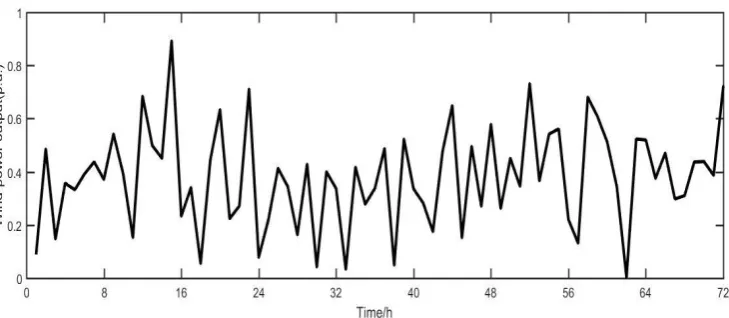
output curve can be obtained. Figure 1 is the annual wind power output variation curve of a certain
169
area. In order to observe its variation more intuitively, the fitting curve is made. Figure 2 is the
170
multi-day wind power output variation curve drawn randomly, and Figure 4 is the typical wind
172
power output curve.
173
Figure 1. Annual wind power output curve
174
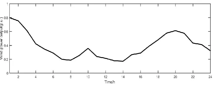
Figure 2. Wind power output curve in different seasons
175
Figure 4. Typical wind power output curve
177
The characteristics of the above wind power output curves are analyzed and summarized as
178
follows:
179
1. Random. As shown in Figure 1, the fitting curve of the annual wind power output curve can be
180
clearly observed. For the hourly statistics of wind power output, the output at each moment
181
shows obvious uncertainty.
182
2. Intermittence. The wind speed has obvious intermittence, and is affected by the cutting-in speed
183
and cutting-out speed of wind turbines, so there are some points in the curve where the output
184
of wind turbines is zero. The point where the output of these fans is zero may be due either to
185
the failure to reach the cut-in wind speed or to the fact that the fan has been removed because
186
the cut-out wind speed has been reached, thus the output of wind power is not continuous.
187
3. Seasonal variation characteristics. As shown in Figure 2, wind power output has a certain
188
seasonal variation characteristics. Wind power output is relatively large in autumn and
189
relatively small in summer, and the difference is relatively obvious. At the same time, the output
190
curve of each season is quite different from the typical solar output curve, and the typical solar
191
output curve can not well reflect the characteristics of output variation in each season.
192
4. Time series characteristics and similarity. It can be seen from the continuous multi-day variation
193
curve and typical sunrise curve that the wind power output has obvious time series
194
characteristics and similarity. The output of wind power is large at night and small at daytime,
195
which has good peak regulation characteristics. The sunrise curve in continuous time has certain
196
similarity, which means that it can reduce the scene effectively.
197
From the above analysis, it can be seen that the wind power output has obvious time series
198
characteristics, and the wind power output has obvious differences with different seasons and
199
different periods of the day. Typical daily method can not adequately express all the information
200
contained in the annual output curve of wind power. At the same time, its contribution has some
201
similarities, which means that it can reduce the necessary scene.
202
2.2.2 Characteristic Analysis of Photovoltaic Output Scene
203
According to the uncertain modeling results of illumination intensity in the previous section,
204
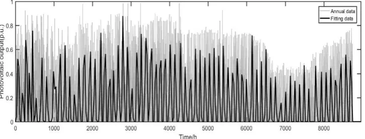
the corresponding photovoltaic output curve can be obtained. Figure 5 is the annual photovoltaic
205
output variation curve and its fitting curve of a region. Figure 6 is the photovoltaic output curve of
206
different seasons. Figure 7 is the continuous multi-day photovoltaic output variation curve. Figure 8
207
is the typical solar output variation curve.
208
Figure 5. Annual wind power output curve
209
Figure 6. Photovoltaic output curve in different seasons
210
Figure 7. Continuous multi-day photovoltaic output curve
211
The characteristics of the above photovoltaic output curves are analyzed and summarized as
213
follows:
214
1. Periodicity. From the solar photovoltaic output curve, it can be clearly observed that the
215
photovoltaic output has obvious periodicity, rising from the morning until about noon to reach
216
the maximum photovoltaic output, and declining in the afternoon. This periodicity is evident in
217
all curves.
218
2. Seasonal variation characteristics. Photovoltaic output is mainly affected by light intensity.
219
Generally speaking, the photovoltaic output is higher in summer than in winter because of the
220
highest illumination intensity.
221
3. Time series characteristics and similarity. From the continuous multi-day curve and typical
222
daily curve, it can be seen that the photovoltaic output changes obviously with time. On sunny
223
days, the continuous multi-day curves sampled randomly have obvious similarities. This also
224
means that the effort scenario can be reduced.
225
From the above analysis, it can be seen that the photovoltaic output has obvious time-series
226
characteristics, and the photovoltaic output has obvious differences with different seasons and
227
intra-day periods. Typical daily method can not adequately express all the information contained in
228
the annual output curve of photovoltaic. At the same time, its contribution also has certain similarity,
229
which means that it can reduce the scene.
230
3. Scene reduction method based on improved clustering algorithm
231
Cluster analysis is a common method for scene analysis in DG planning process. Cluster
232
analysis grouped the same or similar scenarios in DG and load output scenarios, and obtained the
233
classes of similar elements. Clustering algorithm has been widely used in data analysis. For
234
different sets, different classes are needed, so the clustering algorithm has been improved from the
235
corresponding aspects in the specific application at this stage. In this section, we will introduce the
236
common clustering algorithms. In view of the shortcomings of clustering algorithms and the set of
237
scenarios used in this paper, we propose a kind of improved clustering algorithm.
238
3.1. Improved clustering algorithm
239
According to the scenario characteristics of two kinds of DGs, it can be seen that the number of
240
scenario sets in the whole year is large and has certain similarities. Through the introduction of
241
related scene reduction methods, this paper chooses clustering algorithm to reduce the annual
242
scene set. Intra-class similarity and inter-class difference are the criteria for evaluating clustering
243
algorithm. In order to test the clustering results effectively, this paper chooses BWP index to test the
244
clustering results to judge the reliability of clustering scenarios. This index can also give the optimal
245
number of clustering that traditional clustering algorithm can not give.
246
Let𝐾 = {𝑋, 𝑅} be the clustering space, 𝑋 = {𝑥1. 𝑥2, … , 𝑥𝑛}, Assuming that n objects are
247
eventually clustered into class c, the minimum distanceb(j, i)of the sample i in class j is the
248
minimum average distance from the sample to all other types of samples, such as equation 8:
249
𝑏(𝑗, 𝑞) = 𝑚𝑖𝑛1≤𝑘≤𝑐,𝑘≠𝑗( 1 𝑛𝑘
∑‖𝑥𝑝 (𝑘)
− 𝑥𝑖(𝑗)‖2) 𝑛𝑘
𝑝=1
(8)
Where xi(j) is the sample i in class j; xp (k)
is the sample p in class k; nk is the number of samples in
250
class k; and ‖ ‖2 is the square Euclidean distance.
251
The intra-class distance w (j, i) of the sample i in class j is the average distance from the sample
252
to all other samples in class j, such as equation 9:
253
w(i, j) = 1
nj− 1 ∑ ‖xq (j)
− xi(j)‖2 nj
q=1,q≠i
Wherexq (j)
is the sample q in class j, and q ≠ i, nj is the number of samples in class j.
254
𝑏𝑎𝑤(𝑗, 𝑖) is the sum of the minimum class-to-class distance and the intra-class distance of the
255
sample:
256
𝑏𝑎𝑤(𝑗, 𝑖) = 𝑏(𝑗, 𝑖) + 𝑤(𝑗. 𝑖) (10)
𝑏𝑠𝑤(𝑗, 𝑖) is the difference between the minimum class-to-class distance and the intra-class
257
distance of the sample:
258
𝑏𝑠𝑤(𝑗, 𝑖) = 𝑏(𝑗, 𝑖) − 𝑤(𝑗. 𝑖) (11)
The index 𝐵𝑊𝑃(𝑗, 𝑖) of the sample i in class j is the ratio of the clustering distance to the
259
clustering distance of the sample:
260
BWP(j, i) =bsw(j, i) baw(j, i)=
b(j, i) − w(j, i)
b(j. i) + w(j, i) (12)
According to the definition of BWP index, the bigger the value of BWP index is, the better the
261
clustering result is. The average value of BWP index can reflect the quality of clustering results.
262
When the average value of BWP index is the largest, k is the optimal clustering number. avgBWP(k)
263
is used to represent the average value of BWP indices of all samples when data set D is clustered into
264
k class, and kopt is used to represent the optimal clustering number.
265
𝑎𝑣𝑔𝐵𝑊𝑃(𝑘) =1
𝑛∑ ∑ 𝐵𝑊𝑃(𝑗. 𝑖) 𝑛𝑖
𝑖=1 𝑘
𝑗=1
(13)
𝑘𝑜𝑝𝑡= 𝑎𝑟𝑔𝑚𝑎𝑥2≤𝑘≤𝑛{𝑎𝑣𝑔𝐵𝑊𝑃(𝑘)} (14)
BWP index is used to improve the maximum and minimum distance K-means algorithm, and
266
the best clustering result is determined according to the BWP value. The improved algorithm steps
267
are as follows:
268
1. Choosing a center according to the maximum and minimum distance criterion described above
269
2. Clustering according to K-means clustering method based on maximum and minimum distance
270
3. Calculate the BWP value of the clustering result and turn to step 2
271
4. Comparing the BWP value of clustering results, the K value of clustering results is the best
272
clustering number when the BWP value is maximum
273
5. Clustering results corresponding to the maximum output BWP value
274
It should be pointed out that when the scene reduction method based on improved clustering
275
algorithm is used to reduce the specific scene, the reduced scene with larger BWP value can be
276
selected according to the actual scene reduction requirement rather than the maximum value.
277
Choosing the reduced set corresponding to the high K value can make use of the time series
278
characteristic of retaining the original scene set to a greater extent.
279
3.2. Validity test
280
3.2.1 Scene Reduction Process Based on Improved Clustering Algorithm
281
Scene reduction is the process of classifying and merging objects to be clustered. According to
282
the results of past research and the analysis of scenario characteristics in Chapter 2, the wind farm
283
scenic set is divided into four scenarios in spring, summer, autumn and winter. The photovoltaic
284
scenic set is divided into 12 scenarios in spring, summer, autumn, winter and three weather types:
285
cloudy, sunny and rainy. When scene reduction of DG is carried out, scene reduction is carried out
286
with day as the basic unit of clustering. Assuming that the total number of individual
287
scenariosn(1,2, … , N) is N. A single scenario has T-period scenario data. The data contained in all
288
scenarios can be represented by matrix N ∗ T. By improving the clustering algorithm to merge the
289
obtained after reduction have the same temporal characteristics as the original scenes, so as to ensure
291
the temporal characteristics of the scenes before reduction. Scenario reduction of two types of DGs
292
and loads is carried out by using the above method. This paper takes the wind power generation
293
scenario as an example to test the effectiveness of the improved clustering algorithm proposed.
294
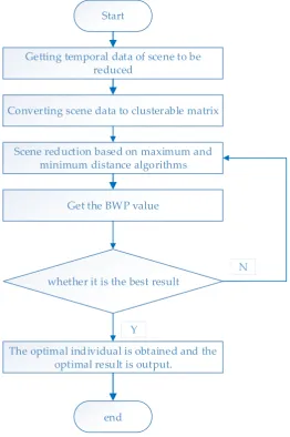
The scene reduction process based on improved clustering algorithm is shown in Figure 9.
295
Start
Getting temporal data of scene to be reduced
Converting scene data to clusterable matrix
Scene reduction based on maximum and minimum distance algorithms
whether it is the best result
end
The optimal individual is obtained and the optimal result is output.
Get the BWP value
N
Y
Figure 9. Reduced flow chart
296
3.2.2. Validity Test of Wind Power output
297
In this paper, wind power generation scenarios are taken as an example to verify the
298
effectiveness of the reduced scenarios. According to the four seasons of spring, summer, autumn
299
and winter, all scenes are divided. The improved clustering algorithm proposed in this paper is
300
used to reduce the partitioned scenes, and the BWP value of clustering results is calculated to select
301
the optimal result.
302
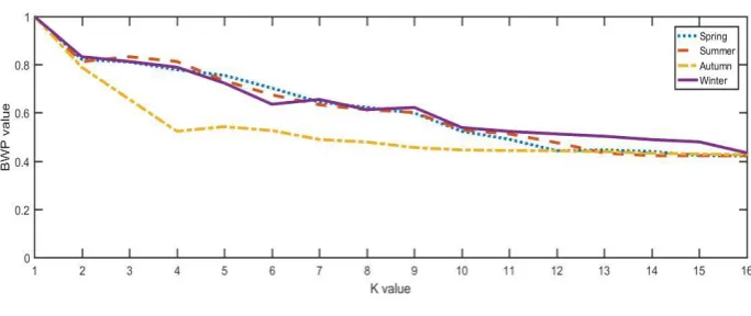
Figure 10. BWP Value Change Curve
304
According to the change curve of BWP value, the BWP value is the largest in spring, autumn
305
and winter scenarios when k = 2, and in summer, when k = 3, the BWP value is the largest. But in
306
order to reflect the temporal characteristics of the original scene to the greatest extent, this paper
307
chooses the case where the K value is relatively large and the number of scenes is relatively large.
308
Taking spring as an example, when k = 2 and K = 5, the K value is larger. Choosing k = 5 here, the
309
scenarios to be reduced are divided into five categories. The output curves of these five scenarios
310
are given below, as shown in Figure 11.
311
Figure 11. Spring Output Curve at k=5
312
According to the law of large numbers, the corresponding probability of each scene at k=5 is
313
shown in Table 1.
314
Table 1. The probability of typical temperatures throughout one year
315
Season
Scene reduction
1 2 3 4 5
Spring 0.57 0.21 0.07 0.12 0.03
In order to reflect the relationship between the reduced scene and the original scene more
316
clearly, scene No. 5 is selected, and two scenes are randomly selected from the reduced scene set for
317
Figure 12. Scene reduction contrast graph
319
According to the reduced output, nearly half of the wind power output in Figure 11 is as
320
shown in Scenario 1. In the other scenarios, the wind power output shows obvious peak reversal
321
characteristics. In the second chapter of this paper, the intra-day variation characteristics of wind
322
power output obtained from scenario characteristics analysis are better reflected in different
323
reduced scenarios. Through the verification of BWP value, and from Figure 12, we can see that the
324
reduced scene obtained by the improved clustering algorithm in this paper has better coincidence
325
with the original scene and can better reflect the temporal characteristics of the original scene.
326
3.2.3. Scene Reduction for Two Kinds of Intermittent DG
327
The scene reduction method based on improved clustering algorithm is used to reduce the
328
output curves of two kinds of DGs, and the validity test is carried out. The results of scene
329
reduction are given directly here.
330
𝛿𝑖(𝑡) = 𝑃𝑤𝑎𝑣(𝑡)/𝑃𝑇 (15)
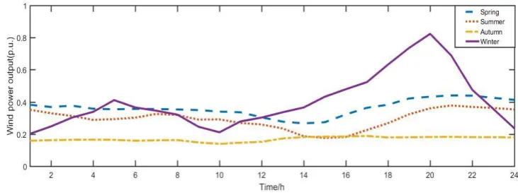
After reducing and normalizing the wind generator scenes divided by seasons, the typical
331
daily scenes are shown in Figure 13.
332
Figure 13. Wind power curve after scene reduction
333
After reducing and normalizing the photovoltaic power generation scenarios divided by
334
Figure 14. Photovoltaic curve after scene reduction in spring
336
Figure 15. Photovoltaic curve after scene reduction in summer
337
Figure 16. Photovoltaic curve after scene reduction in autumn
338
Figure 17. Photovoltaic curve after scene reduction in winter
339
4. Bi-level Programming Model for Distributed Generation Optimal Configuration
340
In the existing DG planning model, the influence of active management mode on distribution
341
network planning is generally considered. However, the ADN active control is generally not
342
considered in the model to maintain the safe and stable operation of islands under the failure state.
343
comprehensive cost. In the upper-level planning, ADN operation strategy in fault scenario is
345
considered, and the comprehensive safety index is introduced and converted into upper-level
346
constraints. To minimize the amount of active power cut-off, this paper adopts the following three
347
kinds of active management measures [22].
348
1. Distributed generator output control
349
2. Switching of reactive power compensation
350
3. Adjustment of on load transformer
351
352
4.1. Upper level programming model
353
The upper-level programming model considers DG layout and installation capacity planning.
354
The objective function is to minimize the annual life cycle investment cost.
355
minC1= CI+ COM+ CP+ CAM+ CL (16)
The specific expressions of each cost are as follows:
356
1. DG Equivalent Investment Annual Cost
357
CI= ( ∑ CWTG,iSWTG,i+ ∑ CPVG,iSPVG,i) r(1 + r) y
(1 + r)y− 1 Nbus
i=1 Nbus
i=1
(17)
Where𝑁𝑏𝑢𝑠is the number of nodes in the distribution network, r is the discount rate, y is the life
358
span of DG for 20 years,𝐶𝑊𝑇𝐺,𝑖and 𝐶𝑃𝑉𝐺,𝑖are fixed investment costs of unit capacity of wind power
359
and PV installed at the i node respectively, 𝑆𝑊𝑇𝐺,𝑖and 𝑆𝑃𝑉𝐺,𝑖are the rated capacity of wind power
360
and PV installed at the i node respectively.
361
2. DG annual operation and maintenance costs
362
𝐶𝑂𝑀 = ∑ 𝑝𝑛× 365(∑( ∑ 𝐶𝑊𝑇𝐺,𝑖𝐸𝑊𝑇𝐺,𝑖𝑛(𝑡) + ∑ 𝐶𝑃𝑉𝐺,𝑖𝐸𝑃𝑉𝐺,𝑖𝑛(𝑡))) 𝑁𝑏𝑢𝑠 𝑖=1 𝑁𝑏𝑢𝑠 𝑖=1 24 𝑡=1 12 𝑛=1 (18)
Where 𝑃𝑛is the scenario probability of the n scenario, 𝐶𝑊𝑇𝐺,𝑖and𝐶𝑃𝑉𝐺,𝑖are the operation and
363
maintenance costs of the wind power and the photovoltaic unit electricity received by the i
364
node,𝐸𝑊𝑇𝐺,𝑖𝑛(𝑡) and 𝐸𝑃𝑉𝐺,𝑖𝑛(𝑡)are the wind power received by the i node and the photovoltaic unit
365
electricity generated during the t period of the n typical day respectively.
366
3. Annual Electricity Purchase Cost
367
CP= ∑ Pn× 365(∑ EntPt) 24
t=1 12
n=1
(19)
Where Entis the t time of n typical days to buy electricity from a higher power grid.Pt is the unit
368
cost of operators purchasing electricity from a higher power grid.
369
4. DG annual active management cost
370
𝐶𝐴𝑀= ∑ 𝑝𝑛× 365(∑( ∑ 𝐶𝐴𝑊𝑇𝐺,𝑖𝐸𝑊𝑇𝐺,𝑖𝑛(𝑡) + ∑ 𝐶𝐴𝑃𝑉𝐺,𝑖𝐸𝑃𝑉𝐺,𝑖𝑛(𝑡))) 𝑁𝑏𝑢𝑠 𝑖=1 𝑁𝑏𝑢𝑠 𝑖=1 24 𝑡=1 12 𝑛=1 (20)
Where CAWTG,i
and
CAPVG,i are the active management costs of the wind power and the371
photovoltaic at the i node respectively.
372
5. Network Loss Cost
373
CL= ∑ Pn× 365(∑ QntLPntL 24
t=1 12
n=1
) (21)
Where 𝑄𝑛𝑡𝐿 is the net loss of the n typical day t period,𝑃𝑛𝑡𝐿is the unit network loss cost.
374
1. DG Installation Capacity Limitation
376
0 ≤ RWTGi≤ RWTGmax
0 ≤ RPVGi≤ RPVGmax
(22)
Where 𝑅𝑊𝑇𝐺𝑖and 𝑅𝑃𝑉𝐺𝑖are the wind capacity and PV capacity node i respectively.𝑅𝑊𝑇𝐺𝑚𝑎𝑥and
377
𝑅𝑃𝑉𝐺𝑚𝑎𝑥correspond to the maximum access capacity of DG respectively.
378
2. Capacity Limitation of DG Total Installation
379
∑ RWTGi+ ∑ RPVGi ≤ RDGmax NPVG
i=1 NWTG
i=1
(23)
Where 𝑅𝐷𝐺𝑚𝑎𝑥 is the maximum installed capacity.
380
3. Constraints of Comprehensive Safety Indicators
381
Ccsi= 1 2(
1
NTS∑ ∑ ∑ Cn,t,s+ min{ S
s=1 T
t=1 N
n=1
Cn,t,s}) (24)
Where Cn,t,s is the index of safe power supply rate of branch s of the n scenario at t period.
382
Cn,t,s= 1 −
∑tt=1T ∑y∈φntfγySn,t,y∆Tn,t,y ∑ ∑i∈φntlγySn,t,y∆Tn,t
tT
t=1
(25)
Where tT is the period of system failure elimination. φntf is the n scenario of t period outage load
383
set.γy is the grade factor of Class y load. Sn,t,y is the Capacity of Class y Load. ∆Dn,t,y is the
384
outage time of y-load in the nth scenario at t period. 𝜑ntl is t period load set for the n scenario.
385
4.2. Lower level programming model
386
The lower level planning model mainly considers the operation constraints related to the
387
operation of distribution network. At this stage, DG access to power grid costs higher. In order to
388
maximize the utilization of DG, the lower level objective is to minimize the amount of active power
389
cut-off of DG, and its expression is as follows:
390
391
𝑚𝑖𝑛𝐶2= ∑ 𝑃𝑛× 365(∑ 𝑃𝑐𝑛𝑡) 24
𝑡=1 12
𝑛=1
(26)
The constraints are:
392
1. Node Power Balance Constraints
393
Pci,i,t,n+ Pco,i,t,n− PWTG,i,t,n− PPVG,i,t,n=
Ui,t,n ∑ Uj,t,n(Gijcos θt,n,ij+ Nbus
j=1
Bijsin θt,n,ij) (27)
Qci,i,t,n+ Qco,i,t,n− QWTG,i,t,n− QPVG,i,t,n− Qc,i,t,n=
Ui,t,n ∑ Uj,t,n(Gijsin θt,n,ij− Nbus
j=1
Bijcos θt,n,ij) (28)
Where 𝑃𝑊𝑇𝐺,𝑖,𝑡,𝑛 and 𝑃𝑃𝑉𝐺,𝑖,𝑡,𝑛 are the active output of the t time of the n scenario,
394
respectively.𝑃𝑐𝑖,𝑖,𝑡,𝑛and 𝑃𝑐𝑜,𝑖,𝑡,𝑛are the active power of residential and commercial loads at the first
395
time of t in the first n scenario, respectively.𝑄𝑊𝑇𝐺,𝑖,𝑡,𝑛and𝑄𝑃𝑉𝐺,𝑖,𝑡,𝑛are the reactive power of DG at
396
the t time of the n scenario, respectively.Qci,i,t,n andQco,i,t,nare the reactive power of resident load
397
reactive power and commercial load at the t time of the n scenario, respectivelyis reactive power
398
supplied by reactive power compensation device.𝑈𝑖,𝑡,𝑛and 𝑈𝑗,𝑡,𝑛 are the voltage amplitude of node i
and the voltage amplitude of node j at the t time node of the n scenario, respectively. 𝜃𝑡,𝑛,𝑖𝑗 is the
400
phase difference between node i and node j of t in the n scenario, respectively.
401
2. Node Power Balance Constraints
402
Uimin≤ Ui≤ Uimax (29)
Where
𝑈
𝑖 is node voltage.𝑈
𝑖𝑚𝑖𝑛and 𝑈𝑖𝑚𝑎𝑥 are the minimum voltage values and maximum403
voltage values allowed by node i respectively.
404
3. Branch power constraints
405
Si ≤ Simax (30)
Where 𝑆𝑖 is the apparent power of branch L. 𝑆𝑖𝑚𝑎𝑥is the limit of branch transmission capacity.
406
4. DG output control constraints
407
Pimin≤ Pi ≤ Pimax (31)
Where𝑃𝑖𝑚𝑖𝑛 and 𝑃𝑖𝑚𝑎𝑥are the minimum active power output of node i and the maximum active
408
power output of distributed generation respectively.
409
5. Constraints of reactive power compensation
410
Qimin≤ Qi≤ Qimax (32)
Where 𝑄𝑖𝑚𝑖𝑛and 𝑄𝑖𝑚𝑎𝑥are the minimum value of reactive power compensation device of node I
411
and the maximum value of reactive power compensation device.
412
6. Regulation constraints of on-load tap-changer
413
Timin≤ Ti≤ Timax (33)
Where 𝑇𝑖is the tap position of transformer i. 𝑇𝑖𝑚𝑖𝑛and𝑇𝑖𝑚𝑎𝑥are the tap values of transformer i and
414
the maximum tap value of i respectively.
415
5. Bi-level Programming Model Solving Algorithms
416
The solution of mixed non-integer programming problem is a common problem in the process
417
of optimal allocation of distributed power supply, and its essence is NP-hard problem. At present,
418
heuristic algorithm and deterministic algorithm are the main solving methods. Particle swarm
419
optimization (PSO), genetic algorithm (GA) and related improved algorithms are widely used in
420
DG programming. In this paper, cuckoo search algorithm is used to solve the upper model, and the
421
lower model is solved by the original dual interior point method.
422
5.1. Cuckoo Search Algorithms
423
Cuckoo search algorithm was first proposed in 2009 by Professor Xin-She Yang and S. Deb of
424
Cambridge University. CS algorithm can efficiently search the optimal solution of the problem by
425
simulating the parasitic brooding of some species of cuckoo. At the same time, CS also uses the
426
relevant Levy flight search mechanism.
427
In the process of cuckoo reproduction, the nest location of cuckoo's offspring is uncertain. In the
428
process of simulating its search for bird's nest, three principles need to be recognized:
429
1. Cuckoos lay only one egg at a time of reproduction, and then they choose their nests arbitrarily
430
for hatching and rearing.
431
2. The most suitable nest will be extended to the next generation of reproduction in a randomly
432
selected set of options.
433
3. The total number of nests available N is a fixed value, and the probability that the original
434
owner of the nest has 𝑃𝑎∈ [0,1] can identify a non-self-laid bird's egg.
435
Based on these three principles, the path and location of cuckoo nest selection are determined
436
xie+1= xie+ α ∗ L(λ), i = 1,2, … , n (34)
Where, xie is the position of the i nest in the selection of the e generation; ∗ is point-to-point
438
multiplication; α is the step size control in the process of choosing nests for cuckoos, which obeys
439
the normal distribution; L(λ) is the path through which Levy searches bird's nest arbitrarily, and
440
L(d, λ)~s−λ(1 < λ ≤ 3), d is the random step obtained by Levy's flight.
441
5.2. Bi-level Programming Model Solving Process
442
The detailed flow chart of solving multi-objective bi-level programming model by CS algorithm
443
Start
Read in system data
The number of iterations G = 0
Initialization of upper population
By introducing relaxation variables, inequality constraints in the lower level programming model are
transformed into equality constraints.
The partial derivative of Lagrange function is 0 for all variables and multipliers, and the nonlinear equation is obtained. The active
output of DG is obtained by solving the equations.
Whether to find heterogeneous
end
Calculate the objective function value of each individual's corresponding planning scheme and calculate the fitness of all
individuals.
Priority of Individuals
Whether the termination condition is satisfied or not
The optimal individual is obtained and the optimal result is output.
Host birds abandon their nests
G=G+1 Choose abandoned bird
nests
Levy flight generates new individuals
N
Y
N
Y
Figure 18. Bi-level planning model solving process
445
6. Examples and Analysis of planning Results
446
0 1 2 3 4 5 6 7 25 13 12 14 11 10 9 8 19 30 24 23 18 31 22 28 29 27 26 21 20 16 15 17 32
Figure 19. IEEE-33 node distribution system.
448
The system voltage is 12.66 kV, total active load is 3.715 MW, total reactive load is 2.300 MW,
449
Weibull distribution parameter k = 2.30, C = 8.92, wind power access cost 6500 yuan/kW, operation
450
and maintenance cost 0.3 yuan/ kW∙h, environmental protection subsidy 0.1 yuan/ kW∙h, rated
451
lighting intensity of photovoltaic generator is 1 kW/m2, shape parameter B of beta distribution is
452
0.85, photovoltaic access The cost is 10,000 yuan/kW, the operation and maintenance cost is 0.2 yuan/
453
kW∙h, the rated capacity of a single distributed power supply is 125 kW, the equipment life is 20
454
years, and the discount rate is 0.1. The repair time of N-1 fault is 4 hours, and the comprehensive
455
safety index value is set to 0.5. Wind power installation nodes are 5, 7, 11, 12. The photovoltaic
456
installation nodes are 20 and 23.
457
6.2. Result analysis
458
On the premise of considering comprehensive safety constraints, the installation types, capacity
459
and cost of distributed generators are compared when the active management mode and the active
460
management mode are taken into account in the lower level planning model. The results are shown
461
in Table 2. Active power removal of lower target in each season is shown in Table 3.
462
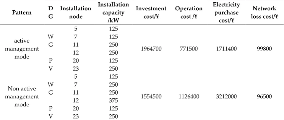
Table 2. Optimal allocation schemes with and without active management.
463
Pattern D G Installation node Installation capacity /kW Investment cost/¥ Operation cost/¥ Electricity purchase cost/¥ Network loss cost/¥ active management mode W G
5 125
1964700 771500 1711400 99800
7 125
11 250
12 250
P V
20 125
23 250
Non active management
mode
W G
5 125
1554500 1126400 3212000 96500
7 250
11 250
12 375
P V
20 125
23 250
The installation capacity of DG configuration scheme is 1125 kW when considering active
465
management mode, which is less than 1375 kW when not considering active management mode. On
466
the premise that the comprehensive security index of the system is taken into account to ensure the
467
safe and stable operation of the system, the active management mode can reduce the amount of DG
468
access. This is because the active management method can actively cooperate with the DG operation
469
according to the actual operation of the system, the tap-in of on-load voltage regulator and the
470
switching of reactive power compensation, so that the system can achieve the optimal operation
471
state at each moment. At this stage, DG access costs are higher, and reducing DG access can reduce
472
the annual life cycle investment costs.
473
Table 3. The excision amount of active output with and without active management.
474
DG removal volume in different seasons(MW∙h)
Spring Summer Autumn Winter
Active management
mode
8.21 3.24 12.15 22.17
Non active management
mode
22.50 15.63 33.21 41.54
475
According to Table 3, the amount of active power removal in different seasons is smaller when
476
subjective management mode is taken into account than when active management mode is not
477
taken into account. In summer when the load level is high, the DG output connected to the
478
distribution network can be basically absorbed. Therefore, the introduction of active management
479
measures improves the utilization rate of distributed energy, and plays a more obvious role in
480
improving the phenomenon of "wind abandonment" and "light abandonment".
481
On the premise of considering active management, the installation type, capacity and cost of
482
distributed generators with comprehensive safety index and without comprehensive safety index
483
are compared. The results are shown in Table 4.
484
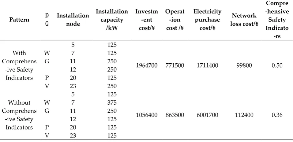
Table 4. Optimal allocation schemes with and without comprehensive safety index.
485
Pattern DG Installation node Installation capacity /kW Investm -ent cost/¥ Operat -ion cost/¥ Electricity purchase cost/¥ Network loss cost/¥ Compre -hensive Safety Indicato -rs With Comprehens -ive Safety Indicators W G
5 125
1964700 771500 1711400 99800 0.50
7 125
11 250
12 250
P V
20 125
23 250
Without Comprehens -ive Safety Indicators W G
5 125
1056400 863500 6001700 112400 0.36
7 375
11 250
12 125
P V
20 125
23 125
486
Without considering the constraints of comprehensive security indicators, the access capacity of
487
the upper model in this paper aims at minimizing the annual cost. Without considering the security
489
constraints, the scheme will tend to have fewer DGs with higher access costs.
490
491
The scheme with comprehensive security index constraints, whose index value is 0.50, and the
492
scheme without comprehensive security index constraints, whose index value is 0.36.When the
493
system is not connected to DG. Without considering the constraints of comprehensive security
494
indicators, the access of DG has little effect on improving the island operation capability of ADN
495
under fault condition. At present, the main function of DG access to distribution network is to
496
improve the operation of the system. Therefore, considering the comprehensive safety indicators, it
497
has obvious effect on improving the operation status of the system in the case of failure in the
498
planning process.
499
On the premise of considering both comprehensive security indicators and active management
500
mode, the economic and technical comparison of DG optimal allocation under the annual time series
501
scenarios, typical day scenarios and reduced scenarios is made. Full-time scenarios are selected as
502
benchmarks to test the planning schemes under the other two scenarios. The annual average of each
503
period is selected as the data of typical day scenes. A summary of the three plans is shown in Table 5.
504
Table 5. Comparison of three kinds of scene set planning schemes.
505
Pattern DG Installati on node
Installation capacity /kW
Annual life cycle investment
cost/¥
Active power excision/
MW∙h
Computing time/s
Annual Sequence
Scene
WG
5 125
5123600 48.26 1803
7 125
11 375
12 250
PV 20 125
23 250
Typical Day Scene
WG
5 125
6145600 31.48 8
7 125
11 250
12 125
PV 20 125
23 125
Scene Reduction
WG
5 125
4547400 45.77 60
7 125
11 250
12 250
PV 20 125
23 250
506
From the comparison results of three scenario planning schemes, it can be concluded that:
507
Most directly, when using reduced scene set for DG planning, the computational time is
508
reduced from about 1803 seconds to only about 60 seconds, and the computational efficiency has
509
been significantly improved. Although the time spent in DG planning using reduced scene sets is
510
slightly longer than that using typical day scenes, the calculation accuracy is higher. In this paper,
511
DG with fixed capacity is used to access the corresponding nodes. Under this assumption, the DG
512
access capacity in reduced scenarios is the same as that in annual sequential scenarios, and the
513
typical daily scenario with average value is smaller than the other two scenarios. Compared with the
514
typical Japanese method, the annual comprehensive cost and the amount of effective removal of
515
reduced scenes are closer to the annual time series scenes. In DG planning process, the access
516
summary, the scene reduction method based on improved clustering algorithm proposed in this
518
paper has better retention effect for the original scene time series data, and the economic and
519
technical indicators can basically accurately reflect the sequence status of the scene before reduction.
520
7. Conclusions
521
The main work of this paper is to use scenario reduction multi-scenario analysis method to
522
optimize the allocation of distributed power in active distribution network. The main problem of
523
this paper is how to take account of both computational efficiency and accuracy in DG planning
524
process by using multi-scenario analysis method, and how to fully consider the active management
525
mode of ADN and the operation status under failure state. Based on uncertainty modeling and
526
scenario reduction, a DG bi-level programming model for active distribution network is constructed.
527
Through the simulation and verification of the IEEE-33 node system, the specific contents are as
528
follows:
529
1. The uncertain modeling of two kinds of DGs is introduced. The scene characteristics of DGs are
530
analyzed. The analysis shows that both kinds of DGs have obvious uncertainties and time series
531
characteristics. Therefore, the typical scenes composed of average method or peak-valley
532
difference maximum sunrise force can not effectively reflect the characteristics of DG, and the
533
two kinds of DG's output scenes are similar and can be effectively reduced.
534
2. Aiming at the shortcomings of clustering algorithm for large-scale scenarios, a scene reduction
535
method based on improved clustering algorithm is proposed and applied to DG planning
536
process. The effectiveness of this method is verified through wind power generation scenarios.
537
3. Through specific examples, the planning schemes considering active management mode and
538
not considering active management mode under the constraints of comprehensive safety
539
indicators, the planning schemes considering comprehensive safety indicators constraints and
540
not considering comprehensive safety indicators constraints under the active management
541
mode, and the planning schemes under three scenarios are compared accordingly. The results
542
show that the active management mode can reduce DG access and annual comprehensive cost
543
while maintaining the stable operation of the system; the introduction of comprehensive
544
security indicators can improve ADN operation capability in the DG planning stage; the
545
planning schemes under three scenarios set show that using the scenario reduction method
546
proposed in this paper. The scene constructed by this method has a good effect on preserving
547
the original scene, and can take account of both computational efficiency and accuracy.
548
Author Contributions: All authors contributed to the research. Conceptualization, Sitong Lv; Data curation,
549
Yongxin Guo; Formal analysis, Sitong Lv and Zhong Shi; Project administration, Jianguo Li; Writing – original
550
draft, Sitong Lv; Writing – review & editing, Sitong Lv.
551
Funding: This work is supported by the Scientific Research Projects of Shanghai Science and Technology
552
Commission (Grant Nos.17DZ1201200).
553
Conflicts of Interest: The authors declare no conflict of interest.
554
Appendix A
555
Table A. Parameters of 33-bus distribution network.
556
Line data
Access Rd Branch impedance/Ω
First spot number
End point
number Resistance Reactance
1 2 0.922 0.047
2 3 0.493 0.2511
3 4 0.366 0.1864
5 6 0.819 0.707
6 7 0.1872 0.6188
7 8 0.7114 0.2351
8 9 1.03 0.74
9 10 1.044 0.74
10 11 0.1966 0.065
11 12 0.3744 0.1238
12 13 1.468 1.155
13 14 0.5416 0.7129
14 15 0.591 0.526
15 16 0.7463 0.545
16 17 1.289 1.721
17 18 0.732 0.574
2 19 0.164 0.1565
19 20 1.5042 1.3554
20 21 0.4095 0.4784
21 22 0.7089 0.9373
3 23 0.4512 0.3083
23 24 0.898 0.7091
24 25 0.896 0.7011
6 26 0.203 0.1034
26 27 0.2842 0.1447
27 28 1.059 0.9337
28 29 0.8042 0.7006
29 30 0.5075 0.2585
30 31 0.9744 0.963
31 32 0.3105 0.3619
32 33 0.341 0.5302
References
557
1. Mehigan, L.; Deane, J.P.; Gallachoir, B.P.O.; Bertsch, V. A review of the role of distributed generation (DG)
558
in future electricity systems. Energy 2018, 163, 822-836
559
2. Anaya, K.L.; Pollitt, M.G. Going smarter in the connection of distributed generation. Energy Policy 2017,
560
105, 608-617.
561
3. Allan, G.; Eromenko, I.; Gilmartin, M.; Kockar, M.; Mcgregor, P. The economics of distributed energy
562
generation: A literature review. Renew. Sustain. Energy Rev. 2015, 42, 543-556.
563
4. Shi, Z.H.; Liang, H.; Huang, S.J.; Dinavahi, V. Multistage robust energy management for microgrids
564
considering uncertainty. IET. Gener. Transm. Dis. 2019, 13, 1906-1913
565
5. Chen, G.; Lewis, F.L.; Feng, N.; Song, Y.D. Distributed optimal active power control of multiple
566
generation systems. IEEE Trans. Ind Electron. 2015, 62, 7079-7090.
567
6. Tan, Y.S.; Wang, Z.Y. Incorporating unbalanced operation constrains of three-phase distributed
568
generation . IEEE Trans. Power Syst. 2019, 34, 2449-2452.
569
7. Ziari, I.; Ledwich, G.; Ghosh,A. Optimal allocation and sizing of DGs in distribution network. In
570
Proceeding of the IEEE Power and Energy Society General Meeting, Minneapolis , MN, USA, 25-29, July
571
2010; pp. 1-8
572
8. Othman, M.M.; El-Khattam, W.; Hegazy, Y.G.; Abdelaziz, A.Y. Optimal placement and sizing of
573
distributed generators in unbalanced distribution systems using supervised big bang-big crunch method.
574
IEEE Trans. Power Syst. 2015, 30, 911-919.
575
9. Kewat, s.; Singh, B. Modified amplitude adaptive control algorithm for power quality improvement in
576
multiple distributed generation system. IET. Power.Eletrons. 2019, 12, 2321-2329.
577
10. Giri, A.K.; Arya, S.R.; Maurya, R.; Babu, B.C. VCO-less PLL control-based voltage-source converter for
578
11. Shaheen, M.A.M.; Hasanien, H.M.; Mekhamer, S.F.; Talaat, H.E.A. Optimal power flow of power systems
580
including distributed generation units using sunflower optimization algorithm. IEEE Access. 2019, 7,
581
109289-109300
582
12. Zou, K.; Agalgaonkar, A.P.; Muttaqi, K.M. Distribution System Planning With Incorporating DG Reactive
583
Capability and System Uncertainties. IEEE Trans. Sustain. Energy. 2012, 3, 112-123.
584
13. Shen, X.W.; Shahidehpour, M.; Zhu, S.Z.; Han, Y.D.; Zheng, J.H. Multi-stage planning of active
585
distribution networks considering the co-optimization of operation strategies. IEEE Trans. Smart Grid.
586
2018, 9, 1425-1433.
587
14. Li, R.; Wang, W.; Xia, M.C. Cooperative planning of active distribution system with renewable energy
588
sources and energy storage systems. IEEE Access. 2017, 6, 5916-5926.
589
15. Zhao, L.; Huang, Y.X.; Dai, Q.D.; et, al. Multistage active distribution network planning with restricted
590
operation scenario selection. IEEE Access. 2019, 7, 121067-121080.
591
16. Shafik, M.B.; Chen, H.K.; Rashed, G.I.; et, al. Adequate topology for efficient energy resources utilization
592
of active distribution networks equipped with soft open points. IEEE Access. 2019, 7, 99003-99016.
593
17. Li, P.; Zhang, C.C.; Fu, X.P.; et, al. Determination of local voltage control strategy of distributed
594
generators in active distribution networks based on kriging metamodel. IEEE Access. 2019, 7, 34438-34450.
595
18. Du, E.S.; Zhang, N.; Kang, C.Q.; Kroposki, B.; Huang, H.; Miao, M.; Xia, Q. Managing wind power
596
uncertainty through strategic reserve purchasing. IEEE Trans. Power Syst. 2017, 32, 2547-2559.
597
19. Wang, Y.; Zhou, Z.; Botterud, A.; Zhang, K.F. Optimal wind power uncertainty intervals for electricity
598
market operation. IEEE Trans. Sustain. Energy. 2018, 9, 199-210.
599
20. Kaloudas, C.G.; Ochoa, L.F.; Marshall, B.; Majiothia, S.; Fletcher, I. Assessing the feature trends of reactive
600
power demand of distribution networks. IEEE Trans. Power Syst. 2017, 32, 4278-4228.
601
21. Wan, C.; Lin, J.; Song, Y.H.; Xu, Z.; Yang, G.Y. Probabilistic forecasting of photovoltaic genenration: An
602
efficient statistical approach. IEEE Trans. Power Syst. 2017, 32, 2471-2472.
603
22. Zhang, J.T.; Cheng, H.Z.; Wang, C. Technical and economic impacts of active management on