1
Experimental Estimation of Temporal and Spatial Resolution of Coefficient of
Heat Transfer in a Channel Using Inverse Heat Transfer Method
Majid Karami 1, Somayeh Davoodabadi Farahani 2, Farshad Kowsary 1*, Amir Mosavi 3,4*
1 School of Mechanical Engineering, University of Tehran, Tehran, Iran; [email protected] &
2 School of Mechanical Engineering, Arak University of Technology, Arak, Iran;
3 School of the Built Environment, Oxford Brookes University, Oxford OX3 0BP, UK;
4 Kando Kalman Faculty of Electrical Engineering, Obuda University, 1034 Budapest, Hungary;
Abstract
In this research, a novel method to investigation the transient heat transfer coefficient in a channel is suggested experimentally, in which the water flow, itself, is considered both just liquid phase and liquid-vapor phase. The experiments were designed to predict the temporal and spatial resolution of Nusselt number. The inverse technique method is non-intrusive, in which time history of temperature is measured, using some thermocouples within the wall to provide input data for the inverse algorithm. The conjugate gradient method is used mostly as an inverse method. The temporal and spatial changes of heat flux, Nusselt number, vapor quality, convection number, and boiling number have all been estimated, showing that the estimated local Nusselt numbers of flow for without and with phase change are close to those predicted from the correlations of Churchill and Ozoe (1973) and Kandlikar (1990), respectively. This study suggests that the extended inverse technique can be successfully utilized to calculate the local time-dependent heat transfer coefficient of boiling flow.
Keywords: Heat transfer, inverse method, boiling flow, local Nusselt number, time resolution
2 Introduction
Boiling flow of a tube takes place in a variety of equipment such as power plants (steam, solar,
and cooling), chemical industries, refrigeration, and air conditioning systems, rendering accurate
knowledge of this phenomenon important. In a two-phase flow, the relative distribution of the
liquid phase and gas in the tube flow is required to describe the flow. The pattern of boiling flow
in the horizontal and vertical pipes is similar. Their difference lies only in the effect of gravity on
the flow, which tends to remain liquid and gas in the down and above of the channel, respectively.
Many works have been conducted on different criteria of boiling [1-3].
Tibiriça and Ribatski [4] performed experimental tests to study boiling heat transfer of R245a in a
tube. Bodhal [5] studied bubbly boiling flow regime in the channel and determined its wavy
character. In the rectangular narrow channel, Kim and Mudawar [6] found out that in addition to
the convection, nucleate boiling has a considerable result in the boiling heat transfer. Boiling heat
transfer of hydrocarbon fluids in a vertical tube is experimentally studied by Wadekar [7]. He
observed pressure drop had been affected by subcooled boiling in the region where almost the
relative distribution of gas to liquid is close to zero. Aria et al. [8] investigated experimentally heat
transfer of R-134a boiling inside a spiral coiled pipe and realized that when the tube changes from
straight to spiral, as well as the pressure drop, heat transfer is also increased. In addition, there
have been extensive research to understand the effect from adding nanoparticles: Al2O3 water [9],
CuO water [10], and Ag water [11] to fluids in boiling flow. Boudouh et al. [12] studied the boiling
flow with nanofluid in mini channel, finding out that Nusselt number and vapor quality increased
3
efficiency of silver nanoparticle in water flow in micro channel. They used two series of
thermocouples in 0.5mm and 8.5mm from the internal surface channel and calculated local heat
flux by means of measured temperature and Fourier Law. They found out that boiling heat transfer
in the channel entrance was more enhanced. Huang et al. [14] studied transient thermal analysis of
electronic tools under a variable heat flux in a multi-micro-channel evaporator. They considered
two and three-dimensional thermal models. Nonetheless, very few works have been performed,
dedicated to the local time-dependent changes of the Nusselt number and the quality of vapor.
Therefore, it is important to attempt understanding thermal phenomena such as boiling flow.
Keeping these in mind, an inverse method has been developed to estimate time history of local
heat flux input into the fluids in a rectangular channel. The objective in the inverse problem is to
predict the unknown using the temperatures measured within the body. These unknowns [15] can
be temperature, thermal flux, thermal properties, heat source or part of the body's geometry and
inverse design [16].The measured temperature data are with noise, while inverse heat conduction
problems are sensitive to noise. Thus, these problems are ill-posed.
Regularization techniques are utilized to alleviate this problem [17-19]. The inverse problem of
predicting heat flux is a linear problem. One of the regularization methods [20] is the conjugate
gradient method. Farahani and Kowsary [21] estimated local Nusselt number in mini-channel
numerically, utilizing the inverse technique. Giedt [22] investigated variations in the Nusselt
number of the airflow perpendicular to a cylinder using an inverse technique. Abia and Yamazkai
[23] conducted an experiment to investigate changes in heat transfer using an inverse method in a
series of cylinders exposed to airflow. Taler [24] predicted the values of the Nusselt number on
4
The heat transfer in the twisted pipes is investigated using the inverse technique, in the fully
developed laminar flow by Borzoi et al. [25] and in the transitional regime by Cattani et al. [26].
Rouizi et al. [27] predicted the bulk temperature in a mini channel using two inverse techniques.
Closer examination of the boiling phenomenon needs to find a precise distribution of heat flux on
the channel’s surface. To achieve this goal, the inverse technique has been proposed in this study.
This method, a non-intrusive one, which is based on conjugate gradient technique, has been
utilized to predict heat flux into the fluids on heat exchange surface, using K-type thermocouples,
inserted in specific locations within the channel, to measure time history of the temperatures,
therefore, it provides inputs for the inverse procedure. For solving the heat equation, the finite
element technique in ANSYS commercial software has been utilized with inverse algorithm code,
written in ANSYS parametric design language (APDL). The flow with and without phase change
is considered in the channel for investigation. Transient two-dimensional thermal model is utilized
to study the heat flux, surface temperature, Nusselt number, vapor quality, convection number,
and boiling number.
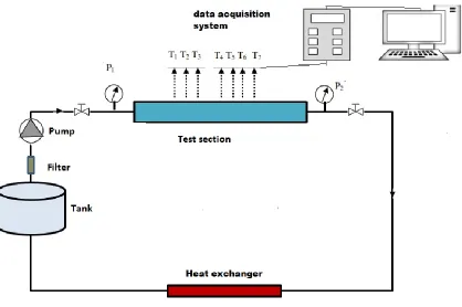
Test Set up
A plan of the test set up in this research is illustrated in figure1. The fluid in the tank is pumped
and the impurities are separated from the fluid by a filter and a regulating valve is employed to set
the mass flux. The uncertainty in the measured flow rate is 5%. In the flow with phase change,
Outflow from the test section is in the two - phase state and before returning to the tank, the heat
5 Figure 1 A schematic diagram of the experiment set up
The test section (Figure 2) is a stainless steel duct, its length is 1.2m. Its cross-section is a rectangle
(40×25 mm2). Each wall, 10 mm thick, is heated by a rectangular heating panel to provide uniform
heating. To reduce heat dissipation, three layers of thermal insulation have been taken into
consideration. The first layer is asbestos with a thickness of 5mm (kasbestos= 0.15 W/ (mK)) which
is directly positioned on the thermal heater; the second layer is fiberglass with a thickness of
30mm (with kfiberglass= 0.04 W/ (mK)) which is applied around the duct; and finally the third layer
is nylon tape (2 mm thick and 50 mm wide with thermal conductivity of 0.25 W/ (mK)) to hold all
the other layers together. These layers of insulation ensure that heat losses are kept below 5%.
The total power of the input heating panels is 3000 W. A power supply has been used to control
6
measured with seven K-type thermocouples, located along the duct at axial distances of 50, 150,
350, 600, 950, 1050, and 1150 mm from the duct inlet. They are placed inside the holes and drilled
into the duct, 0.5 mm from the upper surface.
Figure 2Thermocouple locations in the channel (The dimension is mm)
Table 1 shows the uncertainty associated with measurement of devices, such as flow meters,
thermocouples, heater power, and machining. Applying the proposed method in [28], it is
estimated that the general uncertainty for measuring Nusselt numbers is within the range of 5.8 ±
0.8%.
7
Error source Bias
Thermocouple 0.1°C
Flow meter 5%
Heater power 1%
Machining process 0.02mm
Problem Description
The conjugate gradient technique has been employed to predict heat fluxes into the fluid in a
rectangular channel. The channel is made of AISI 313. The heat flux is equal to the heater power.
Temporal and spatial variations of heat flux and surface temperature at y=E is unknown. It has
been assumed that the loss of heat is negligible with the governing equation of the plate[20],
written as: i E y y w y y L x x t yy xx T y x T k t x q T k q T T T T T ) 0 , , ( ) , ( 0 1 1 0 , 0 1 (1)
Where𝑇𝑖, L, E, and 𝑞𝑤are the initial temperature, length and thickness of plate, and heater power,
respectively. 𝑞(𝑥‚𝑡) is unknown; thus instead of the heat flux, the measured temperatures by the
thermocouples are available from the experimental test. The temperature of the channel wall is
8
predict indirectly the convective heat transfer coefficient (h). First, the 𝑞(𝑥‚𝑡) is estimated and
then ℎ is estimated by using Newton’s cooling law and estimated 𝑞(𝑥‚𝑡). Thus, we modeled the
heat conduction equation (equation (1)) in the channel wall and convection term has appeared in
the boundary condition. This term is unknown. The measured data contains information about ℎ,
which can be achieved by decoding method. The conjugate gradient method as the inverse
technique has been used to retrieve this information. The temperatures are measured inside the
plate using the thermocouples. These measurements are as input in the inverse technique. The most
important point of this technique is that no information is required from the fluid flow field.
Table 2 Thermal property of work material
Thermal property value
Specific heat,𝐶𝑝(J/(kgK)) 460
Thermal conductivity, 𝑘(𝑤/(𝑚𝐾)) 28.6
Density,𝜌(𝑘𝑔/𝑚3 ) 7760
Table 3 Thermocouple position coordinates
Thermocouple no.
X (mm)
Y (mm)
T1 50 -0.5
T2 150 -0.5
T3 350 -0.5
T4 600 -0.5
T5 950 -0.5
T6 1050 -0.5
9
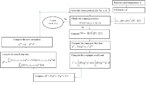
In order that heat equation solving, the Finite-Element Method has been used in ANSYS software.
In the direct thermal problems, all boundary conditions and material properties (Table 2) are
known. Table 3 shows the location of thermocouples within the plate. The inverse method,
conjugated gradient method (CGM), estimates the 𝑞(𝑥‚𝑡), using the temperatures are recorded
from specified positions in the plate. The details of the CGM algorithm has been presented in pervious author’s work [20], thus they will not be brought here. The inverse method employs a
parameter, called the sensitivity coefficient, in fact indicating the temperature sensitivity of the
unknown parameter. The sensitivity coefficient [16] is calculated as:
(2)
Ns m
q t y x T t
y x
X ( m, m, ) ( m, m, ) 1,2,..,
where xm and ym are the sensor location within the channel wall, and P is the number of sensors.
It must be noticed that the number of unknowns should be smaller or equal to the number of
thermocouples in IHCP [15]. No functions have been employed to predict the heat flux
components. One of the principles of inverse heat transfer is that we have no knowledge about the
unknowns. The flow chart of which is illustrated in Figure 3, showing the iterative procedure for
an inverse method. In this study utilizes seven thermocouples. At least one thermocouple is
required to estimate each heat flux component in IHCP [20]. In order to describe heat flux on the
heat exchange surface, this study estimates seven parameters, q1, q2…, and q7 which vary with
time. Error analysis is done to determine the accuracy of the proposed algorithm. As such, this
10 Figure 3 Inverse algorithm
Temperatures, obtained as a result of a known imposed 𝑞𝑒𝑥𝑎𝑐𝑡, are perturbed by a noise with (σ=0.1°C). These temperatures were used to predict the 𝑞 on each interval. Root mean square
error, bias error, and variance error are calculated in error analysis of the inverse technique. The
mean squared error is used to check the accuracy of the estimation. This error [16]is calculated as
N i i noisydata i q q N RMS 1 2 , ) ˆ ( 1 (3)Where qˆi,noisydata is the predicted heat flux. Bias error[16] is because of the regularization method
and can be calculated as follows.
11
In which qˆi,nonoise is estimated using temperatures with 𝜎 = 0.The inverse method's sensitivity to
the measurement errors in the data is called the variance error [16] and can be calculated as:
2 2
D RMS
V (5)
For better comparison, the errors have the same scale, hence the second root of the variance is
used here. It is necessary for every experimental test that an experimental design should be
carried out. This work is also done in this study. In the inverse problem, it is quite clear that the
sensors should be closer to the active surface (i.e. boiling surface) and the accuracy of this
approach is higher due to the high sensitivity coefficient. In this experiment, the temperature
sensors were located at 𝑦 = 𝐸 − 0.5𝑚𝑚 due to the precision of the machining equipment. In
IHCP [21-22], a small time step causes an increase in the variance error and a very large time
step increases the bias error. We are looking for a suitable time step that the RMS error is low
and we can reach more details about the unknown parameter over time. The time step is
determined according to the RMS. The time step is considered 0.01s, 0.05s, 0.1sand 0.5s and
using the numerical simulation experiments, the error is calculated and is equal to values
0.8qmean,0.05qmean ,0.069qmean and 0.072qmean, respectively. According to the results, 0.1 seconds
is selected. It should be noted that the smallness of the sensitivity coefficient has a direct effect
on the increase of RMS error.
Table 4 presents the error analysis for estimated heat flux on the heat exchange surface. Results
show that the proposed method has a low error, estimating heat flux. This error is almost 0.06
qmean. In the proposed method, firstly the 𝑞(𝑥‚𝑡)is predicted and then, using Newton's cooling
law, ℎ is calculated; therefore, the ℎ is estimated indirectly. The proposed algorithm is simple
12 Table 4 Error analysis for the purposed inverse method
Error RMS(W/m2) Bias(W/m2) variance(W/m2)
Estimated heat flux 0.069× qmean 2.4e-14× qmean 0.069× qmean
Results
The ℎ (𝑥, 𝑡)is calculated using the q(x,t), itself estimated by the inverse method(𝑞(𝑥, 𝑡))and the
calculated local surface temperature (𝑇𝑠(𝑥, 𝑡))as follows as:
) , ( ) , ( ) , ( ) , ( t x T t x T t x q t x h f s (6)
Where 𝑇𝑓(𝑥, 𝑡)is the bulk temperature and is calculated, using the energy balance equation:
P f f C m x W H t x q t x x T t x T
( , ) ( , )(2 2 )
) ,
( (7)
In which q and Ts are estimated through solving IHCP, 𝐻 is channel height, and 𝑊 𝑖𝑠 channel
width. The heat transfer coefficient(𝑁𝑢𝑠𝑠𝑒𝑙𝑡 𝑛𝑢𝑚𝑏𝑒𝑟) [2] is specified as follow as:
) 2 ( ) , ( ) , ( W H HW k t x h t x Nu (8)
This study investigates ℎ(𝑥, 𝑡)for flow with and without phase change. Several experiments were
tested in this study. Considering the number of thermocouples and time-steps, millions of
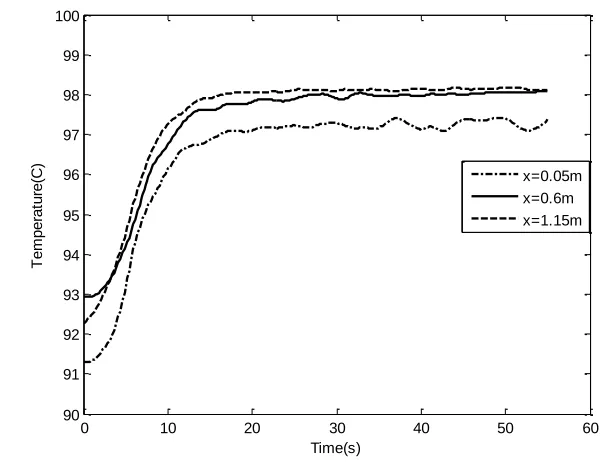
temperatures were acquired as raw data, which we couldn't present here. Figure 4 illustrates the
measured temperatures at each position of the sensor in the flow without phase change (Re=1800)
and in liquid-vapor phase flow G = 355 kg/(m2s). An increase in temperature is observed with
increasing 𝑥.Also,temperature increases over time. As the flow of fluid enters the channel(𝑎𝑡 𝑥 =
0), the thermal boundary layer forms and develops. The Nusselt number in the channel
13
the Nusselt number reduces until the flow (thermal and hydrodynamic) is fully developed. At this
time, the heat transfer coefficient does not change with 𝑥 and is constant. During the two phase
flow, the temperature increases along the channel. First, the temperature increases with the time it
starts to boil and the bubble is generated inside the stream, in this case, the temperature reaches a
constant value. In fact, Measurements emphasize on this issue the essence of the flow inside the
channel strongly affects surface temperature variations.
a)
0 10 20 30 40 50 60
20 30 40 50 60 70 80 90 100
Time(s)
T
e
m
p
e
ra
tu
re
(C
)
14 b)
Figure 4 the measured temperatures a)single phase (Re=1800)and b)two-phase flow(G=355 kg/(m2.s))
Single-Phase Flow
The effect of 𝑅𝑒 changes on 𝑁𝑢(𝑥. 𝑡)in the single-phase flow has been studied. The obtained
results for single-phase flow are validated with Equation (10). Churchill and Ozoe [29] used
experimental results to find a correlation to predict the Nusselt number in a fully developed plug
flow in a pipe with 𝑞 = 𝑐𝑡𝑒. A closed-form expression [29] for the 𝑁𝑢𝑥, covering both the
developing and developed flow in a tube with 𝑞 = 𝑐𝑡𝑒is:
) Pr Re 4 /( ] ) ] ) 6 . 29 / ( 1 [ ] ) 0207 . 0 (Pr/ 1 [ 04 . 19 / ( 1 [ ] ) 6 . 29 / ( 1 [ 364 . 4 3 / 1 2 / 3 3 / 1 2 2 / 1 3 / 2 6 / 1 2 x Gz Gz Gz Gz Nux (9)
For all Gz, this equation agrees within 5% error in developing flow and 3.5% error developed flow
for Pr=0.7 and Pr=10[29]. In calculating the Nusselt number for non-circular cross sections, a
0 10 20 30 40 50 60
15
hydraulic diameter is utilized. In these cross sections, the Wall-Stream effect must be considered
in calculating the Nusselt number based on the hydraulic diameter(𝐷ℎ = 2𝐻𝑊
𝐻+𝑊). This correction [30] is done using the coefficient of 𝛽 = ((𝜋𝐷ℎ2)/4)/𝐴𝑑𝑢𝑐𝑡. Based on the modification of obtained
𝑁𝑢𝑥 extracted from Eq. (9), it could be rephrased as [30]:
x
x Nu
Nu (10)
The importance of β can be seen in Equation (10). Also, Figure (5) illustrates the estimated time
distribution of heat transfer coefficient for Re= 1165 and Table 5 gives difference of
estimated𝑁𝑢 values with the values calculated from Equation (10), showing the highest and
lowest difference to be 18% and 0.4%, respectively. A comparison of the estimated single-phase
Nu with one predicted (eq.10) for laminar flow in rectangular channels is shown in figure 6a,
wherein time-averaged estimated Nu is compared with the values, obtained from Equation (10).
a)
0 10 20 30 40 50 60
0 1 2 3 4 5 6 7 8 9 10
time(s)
Nu
Re=1165
Nu1
Nu3
Nu5
16 b)
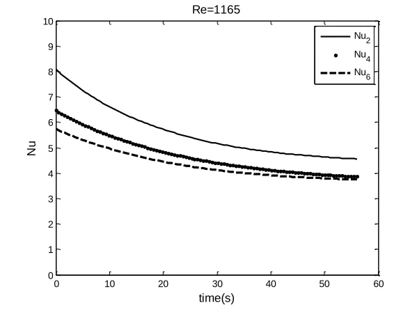
Figure 5 The estimated time history of Nusselt number of single-phase flow for Re=1165
0 10 20 30 40 50 60
0 1 2 3 4 5 6 7 8 9 10
time(s)
Nu
Re=1165
Nu2
Nu4
17
Figure 6 The local Nusselt number along the channel length for a)Re=770,b)Re=1165 and c)Re=1800
At the present work, and the difference of values calculated from the two correlations is about 7
%, and the results are approximately one. Perhaps because the geometry is simple and this affects
the flow structure. The 𝑁𝑢𝑥for Re=770,1165 and 1800 is illustrated in Figure6 . Furthermore,
the averaged deviation percentage of estimated Nusselt number with the results of Equation (10) a)
b)
18
for Re=770, 1165 and 1800 is given in Table 6. The relative deviation is about 2%. Quite
obviously, the reason for the deviations is the method for the prediction of the𝑁𝑢𝑠𝑠𝑒𝑙𝑡 𝑛𝑢𝑚𝑏𝑒𝑟.
Table 6 shows where the predicted values fully agree with equation (10). The mentioned method
has a good accuracy to estimate heat transfer coefficient. It shows that the proposed method can
successfully estimate Nusselt number for flow without phase change.
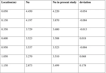
Table 5 Deviation between the extracted Nu from eq.10 and estimated Nu Location(m) Nu Nu in present study deviation
0.050 4.450 4.220 -0.054
0.150 4.197 3.870 -0.084
0.350 3.729 3.680 -0.013
0.600 3.523 3.588 0.018
0.950 3.537 3.523 -0.004
1.050 3.270 3.510 0.068
1.150 2.873 3.499 0.178
Boiling Flow
Table 7 gives the experimental conditions for boiling flow. The mass flux varies between 118.1
and 355 kg/(m2.s), whereas the 𝑞𝑤is from 0 to 19.2 kW/m2. Figure 7shows time variations of the
estimated 𝑞(𝑥, 𝑡)on the heat exchange surface for G=234kg/(m2 s). Nusselt number for boiling
19
Table6 Mean deviation between the estimated Nu and calculated Nu from Equation(10)
Re=1165 Re=1800 Re=770
Equation(10) 3.60 3.78 3.56
estimated 3.64 3.73 3.56
Error 0.011 -0.014 -0.001
Table 7 Mass flux and heat flux for two phase flow
G( kg/(m2.s)) 118.1 234 355
qw(kW/m2) 7.9 14 18.9
20 b)
Figure 7The time history of the local heat flux along the channel length
To compare the Nusselt number of boiling flow inside the tube, it has been applied to the
correlation that Kandlikar [31] has been given. Kandlikar’s correlation [31] is
] ) ( 1058 ) 25 ( 6683 . 0
[ 2 0.3 0.7
2 2 . 0 fg h L sp Gh q gD G Co Nu
Nu
(11)
Where Nusp is Nusselt number in the single-phase state and is calculated by assuming that all flow
inside the channel is liquid and Co is the convection number, defined by [31]:
5 . 0 8 . 0 ) ( ) 1 ( L G v v x x Co (12)
In which 𝑥𝑣. 𝜌𝐿. 𝑎𝑛𝑑 𝜌𝐺 are the local vapor quality, the density of liquid and vapor, respectively.
On average, the deviation of this equation for water and all the refrigerants is about 15.9% and
18.8%, respectively [31]. In order to specify the quality of vapor, the energy equilibrium equation
for every section between the input and the output is employed. The vapor mass qualities [31]is
21 ))] , ( ( ) )( , ( 2 [ 1 ) , ( ) ,
( . x C T T x t
m W H t x q h t x x X t x
X P sat f
fg v
v
(13)
Figure 8a shows the time-averaged Nu decreases with increasing 𝑥 and the experimental results
are close to the predictions of Kandlikar [31]. Near the entrance of channel is the difference
between the estimated values and the reference values [31] at about 19 % and in the rest of the
regions, this difference is insignificant. The reason for this difference between the empirical
correlations with the present work can be attributed to how the heat flux is calculated at the 𝑦 = 𝐸,
in these two empirical correlations the authors have assumed that 𝑞(𝑥. 𝑡) = 𝑞𝑤. Another reason
may be that the curve fitting of the experimental data has errors and the results of the correlation
on the test data are not fully matched.
Time distribution of vapor quality along the channel is illustrated in Figure 8 b. The quality of the
vapor increases in the flow direction along the channel, thanks to the bubble coalescence
mechanism; therefore, the frequency of the bubbles is reduced. This explains why heat transfer is
reduced when the quality of steam is increased. It can be determined when the vapor generation
along channel length starts, as it is one of the findings of the proposed method. The heat transfer
of boiling flow consists of the convective and the nucleate boiling terms. Using the proposed
22 a)
b)
Figure 8 a) the local convective heat transfer coefficient along the channel length, and b) time variation of local vapor quality along the channel length
Figures (9) and (10) demonstrate the variations of 𝐶𝑜 𝑛𝑢𝑚𝑏𝑒𝑟 and 𝐵𝑜 𝑛𝑢𝑚𝑏𝑒𝑟with time.
23
along the channel, which descends as well. The maximum amount of Co corresponds to the 50
mm distance from the channel entrance. Boiling number at the measurement points increases with
time. Temporal and spatial Variations of Boiling number is similar to the variations of the predicted
heat flux. The nucleate boiling heat transfer is dominant when the 𝐶𝑜 number is too large. In the
nucleate boiling region, the 𝑁𝑢 is a weak function of the convection number because the
mechanism of convection has little effect in this area and is not the dominant mechanism. In the
area where the convective boiling mechanism is dominant, the amount of convection number is
small. The contribution of the convective boiling decreases when the Boiling number is increased.
Figure 11 illustrates the variations in the time-averaged of Nusselt number for G = 118.1,234, and
355 kg/(m2.s) with the quality of vapor. As the figure shows the Nusselt number reduces with an
enhancement in 𝑋𝑣. The 𝑋𝑣 is low when the nucleate boiling is dominant. This mechanism and
convective heat transfer help to enhance the heat transfer. The time distribution of local Nusselt
number for G=118.1 kg/(m2.s) is presented in Figure 12. At x = 50 mm the number varies with
24 a)
b)
25 a)
b)
26
27 a)
28
Figure 12 The time variation of local Nusselt number for G=118.1 kg/(m2.s)
Conclusions
This research conducted a laboratory investigation of water flow with and without phase change
in a channel. The temperatures within the wall were experimentally measured, providing the input
data for inverse method to predict theq(x,t). Transient analysis was performed. First, the
experiment was designed and error analysis carried out to determine the accuracy of the proposed
method. RMS error for estimation heat flux was around 0.06qmean. Using Newton's cooling law
and estimated values of heat flux, temporal and spatial distribution of Nusselt number was
predicted. The time-averaged local Nusselt number estimated for flow with and without phase
change were close to those, predicted by the correlations of Churchill and Ozoe [29] and Kandlikar
[31], respectively. It was seen in boiling flow that local quality of vapor and boiling number
increased and local convection number decreased with time. Also, along the length of channel
time-averaged Nusselt number decreased with quality of vapor. The temporal and spatial changes
of the Convective number and the Boiling number can be determined using the proposed method.
29
Nomenclature:
Bo Boiling number, dimensionless
Co Convection number, dimensionless d Conjugate direction used in figure(3) D bias error
G Mass flux, kg/(m2.s)
Gz Graetz number, dimensionless
H height of channel, m
h convective heat transfer coefficient, W/(m2K)
K thermal conductivity, W/ (mK)
E length of plate, m
L thickness of plate, m
N measurements number
Np unknown parameter numbers
Ns sensor numbers
Nu Nusselt number, dimensionless
Nusp single-phase Nusselt number, dimensionless
30
Pr Prandtl number, dimensionless
q heat flux, W/m2
qw Heater’s heat flux, W/m2
Re Reynolds number, dimensionless
RMS root mean square error
T calculated temperatures, K
Tsat saturation temperature, K
Tf, local fluid temperature, K
V variance error
Xv quality of vapor
Y measurements, K
W width of channel, m
Greek Symbols
ρ density, kg.m-3
α thermal diffusivity,m2/s
ε value of noise
search step (figure (3))
31 References
[1] Thome, J.R., El Hajal, J., Two – Phase Flow Pattern Map for Evaporation in Horizontal
Tubes: Latest Version, Heat Transfer Engineering, vol. 24, no. 6, pp. 3-10, 2003.
[2]Frances Viereckl F., Christoph E.S., Wolfgang S., Hurtado,A.L., Experimental and
theoretical investigation of the boiling heat transfer in a low-pressure natural circulation
system, Experimental and Computational Multiphase Flow,Vol.1, Issue 4, pp 286–299,2019.
[3] Kuznetsov V.V.,Fundamental Issues Related to Flow Boiling and Two-Phase Flow Patterns
in Microchannels – Experimental Challenges and Opportunities, Heat Transfer Engineering
Vol. 40, 2019.
[4] Tibiriça, C.B., Ribatski, G., Two-phase frictional pressure drop and flow boiling heat
transfer for R245fa in a 2.32 mm tube, Heat Transfer Engineering, vol. 32, no.13, pp.
1139-1149,2011. DOI: 10.1080/01457632.2011.562725
[5] Bohdal,T., Development Of Bubbly Boiling In Channel Flow, Experimental Heat Transfer,
vol.14,no.3, pp.199–215,2001.
[6] Kim,S., Mudawar,I., Universal approach to predicting saturated flow boiling heat transfer
in mini/micro-channels – Part II. Two-phase heat transfer coefficient, Int. J. Heat Mass Transf.
vol.64,pp.1239–1256, September2013.
[7] Wadekar, V.V., Hydraulic characteristics of flow boiling of hyrdocarbon fluids: two phase
pressure drop, Heat Transfer Engineering, vol. 33, no.9, pp. 786-791, 2012.
[8] Aria, H., Akhavan-Behabadi, M.A., Shemirani, F.M., Experimental Investigation on Flow
Boiling Heat Transfer and Pressure drop of HFC-134a inside a Vertical Helically Coiled
32
[9] Buongiorno,J.,Convective transport in nanofluids, J. HeatTransfer, Trans. ASME, vol.128,
no.3, pp.240-250,2006.
[10] Lee, S., Choi, S.U.S. , Li, S. and Eastman, J.A. , Measuring thermal conductivity of fluids
containing oxide nanoparticles, J. Heat Transfer,vol. 121, no.2,pp.280-289,1999.
[11] Kang, Sh., Wei, W. Ch., Tsai, Sh.H. and Yang, Sh.Y., Experimental investigation of silver
nano-fluid on heat pipe thermal performance, Appl. Therm. Eng., vol.26,pp.2377-2382, December
2006.
[12] Boudouh, M., Gualous, H.L. and Labachelerie, M. De, Local convective boiling heat transfer and pressure drop of nano fluid in narrow rectangular channels, Applied Thermal Engineering,
vol.30, pp.2619-2631, December 2010.
[13] Chehade, A. A., Gualous, H. L., Masson, S. L., Fardoun, F. and Besq, A., Boiling local heat
transfer enhancement in inichannels using nanofluids, Nanoscale Research Letters, vol.8, pp.
130-138, Springer. 2013.
[14] Huang, H., Lamaison N., and Thome, J.R., Transient Data Processing of Flow Boiling Local Heat Transfer in a Multi-Microchannel Evaporator Under a Heat Flux Disturbance , Journal Of
Electronic Packaging,vol.139, pp. 11005-11010, Jan 2017.
[15] Tikhonov, A. N., Inverse Problems in Heat Conduction, J. Eng. Phys., vol.29, pp.816–
820,1975.
[16] Beck, J. V., Blackwell, B. and Clair, C. R. St., Inverse Heat Conduction: Ill-Posed
Problems,Wiley Interscience, New York, 1985.
[17] Babu, K.T. andKumar, S.P., Mathematical modeling of surface heat flux during quenching,
33
[18] Necati Ozisik, M., and Orlande, H. R. B., Inverse Heat Transfer-Foundation and Applications,
Taylor & Francis, USA state, 2000.
[19] Rao, S., Engineering Optimization: Theory and Practice, 3rd Edition, Wiley, 1996.
[20] Farahani, S.D., Kowsary, F.,and Jamili, J.,Direct Estimation Local Convective Boiling Heat
Transfer Coefficient in Mini Channel by Using Conjugated Gradient Method with Adjoint
Equation, International Communication Heat and Mass Transfer, vol.3,pp. 4-10, July2014.
[21] Farahani, S.D.and Kowsary ,F., Estimation Local Convective Boiling Heat Transfer
Coefficient In Mini Channel, International Communications in Heat and Mass Transfer,
vol.39,pp.304-310, February2012.
[22] Giedt, W.H. , “Investigation of variation of point unit heat-transfer coefficient around a
cylinder normal to an air stream”, ASME Transaction, vol. 71, pp. 375-381,1949.
[23] Aiba, S. and Yamazaki, Y., “An experimental investigation of heat transfer around a tube in
a bank”, Journal of Heat Transfer, vol. 98, no. 3, pp. 503-508,1976.
[24] Taler, J., “Determination of local heat transfer coefficient from the solution of the
inverse heat conduction problem”, Forschung im Ingenieurwesen, vol. 71, no. 2, pp.
69-78,2007.
[25] Bozzoli, F., Cattani, L., Rainieri, S., Bazán, F.S.V. and Borges, L.S., “Estimation of the local
heat-transfer coefficient in the laminar flow regime in coiled tubes by the Tikhonov
regularization method”, International Journal of Heat and Mass Transfer, vol.72, pp. 352-361,
34
[26] Cattani, L., Bozzoli, F., Rainieri, S. Experimental study of the transitional flow regime
in coiled tubes by the estimation of local convective heat transfer coefficient, International
Journal of Heat and Mass Transfer, vol.112, pp. 825-836,2017.
[27] Rouizi, Y., Al Hadad, W., Maillet, D., Jannot, Y., Experimental assessment of the fluid
bulk temperature profile in a mini channel through inversion of external surface temperature
measurements, International Journal of Heat and Mass Transfer,vol.83,pp. 522-535,2015.
[28] Kline, S.J., and McClintock, F.A., Describing Experimental uncertainties in single sample
experiment. Mechanical engineering, vol.75,no.1,pp.3-8,1953.
[29] Churchill, S.W.,and Ozoe, H., Correlations for force convection with uniform heating in flow
over a plate and in developing a fully developed flow in a tube, J.Heat
Transfer,vol.95,pp.78-84,1973.
[30] Bejan,A.,convection heat transfer,2013 John Wiley & Sons, Inc., Fourth edition,2013.
[31] Kandlikar, S. G., "A general correlation for saturated two-phase flow boiling heat transfer