Elastic constants from direct correlation functions in nematic liquid crystals: A computer simulation study

Elastic constants from direct correlation functions in nematic liquid

crystals: A computer simulation study

Nguyen Hoang Phuong, Guido Germano, and Friederike Schmid Fakulta¨t fu¨r Physik, Universita¨t Bielefeld, 33501 Bielefeld, Germany

共Received 27 March 2001; accepted 27 July 2001兲

Density functional theories such as the Poniewierski–Stecki theory relate the elastic properties of nematic liquid crystals with their local liquid structure, i.e., with the direct correlation function 共DCF兲 of the particles. We propose a way to determine the DCF in the nematic state from simulations without any approximations, taking into account the dependence of pair correlations on the orientation of the director explicitly. Using this scheme, we evaluate the Frank elastic constants

K₁₁, K₂₂, and K₃₃ in a system of soft ellipsoids. The values are in good agreement with those obtained directly from an analysis of order fluctuations. Our method thus establishes a reliable way to calculate elastic constants from pair distributions in computer simulations. © 2001 American

Institute of Physics. 关DOI: 10.1063/1.1404388兴

I. INTRODUCTION

Nematic liquid crystals are fluids of anisotropic particles, which are aligned preferentially along one direction.1,2Their orientation is characterized by a director n of unit length, with physically identical states n and ⫺n. Since the long range orientational order breaks a continuous symmetry, the isotropy of space, there exist soft fluctuation modes—spatial variations of the director n(r)—which cost no energy in the infinite wavelength limit 共i.e., the limit where n is rotated uniformly兲 and are otherwise penalized by elastic restoring forces.3,4 For symmetry reasons, the latter depend on only three material parameters at large finite wavelengths.1– 6 They are described by an elastic free energy functional6

F兵n共r兲其⫽1

2

冕

dr兵K11关“•n兴

2_⫹K

22关n•共“⫻n兲兴2

⫹K33关n⫻共“⫻n兲兴2其, 共1兲

which has three contributions: the splay, twist, and bend modes. The parameters K_␣␣(␣⫽1,2,3), called Frank elastic constants, control almost exclusively the structure and the properties of nematic liquid crystals at mesoscopic length scales. Expressions that relate them to the microscopic prop-erties of liquid crystals are thus clearly of interest.

Several microscopic approaches have been proposed and employed in the past.7–58 Poniewierski and Stecki35 have used the density functional formalism59 to derive a set of equations which connects the elastic constants with the direct pair correlation function共DCF兲, one of the central quantities in liquid state theories.60,61In a coordinate frame where the z axis points along the director n, the equations read

K11⫽ k_BT

2

冕

rx

2

c共r,u1,u2兲

⫻␳共1兲

_⬘

_共u

1z兲␳共1兲

⬘

共u2z兲u1xu2xdr du1du2, 共2兲

K22⫽ kBT

2

冕

rx

2

c共r,u1,u2兲

⫻␳共1兲

_⬘

_共u

1z兲␳共1兲

⬘

共u2z兲u1yu2ydr du1du2, 共3兲

K33⫽ kBT

2

冕

rz

2

c共r,u1,u2兲

⫻␳共1兲

_⬘

_共u

1z兲␳共1兲

⬘

共u2z兲u1xu2xdr du1du2, 共4兲

where the vector r connects the centers of mass of two mol-ecules 1 and 2, u₁, u₂ are unit vectors along the molecule axes, c(r,u1,u2) denotes the DCF in the nematic liquid, and ␳(1)

_⬘

_(u

z) is the derivative of the one-particle distribution

function with respect to uz. The integrals兰dr run over all

space, and 兰du over the full solid angle, T is the

tempera-ture, and kB is the Boltzmann constant.

Equations of the form 共2兲–共4兲 have later been rederived36 – 46 and applied in theories47–58 and simulations62– 65 to study elastic constants in nematic liquid crystals.66The main difficulty with the Poniewierski–Stecki equations is that they depend on the DCF in the nematic phase, which is not known. Theories have resorted to ap-proximations, e.g., they use a DCF from an effectively iso-tropic reference state,37– 42 or from a state with perfectly aligned particles.29,30,55 Simulation studies62– 65 have ne-glected the explicit angular dependence of the pair correla-tion funccorrela-tions on the orientacorrela-tion of the director. Longa et al. have recently pointed out that this approximation may not be adequate in nematic liquid crystals.67

Alternatively, the elastic constants can also be deter-mined directly from the long-wavelength fluctuations of the order tensor in Fourier space

Q共k兲⫽V

Ni

兺

⫽1

N

共3

2ui丢ui⫺

1

2I兲exp共ik•ri兲, 共5兲

where the sum runs over all particles i in the system, I de-notes the unit matrix and 丢 the dyadic product of two vec-tors. The largest eigenvalue of the 3⫻3 matrix Q at zero

7227

wave vector (Q(k)兩_k⫽0) is the nematic order parameter

V P₂, and the corresponding eigenvector is the director n of the nematic liquid.

In a reference frame where the z axis points along n and the y axis is perpendicular to k, the order tensor fluctuations have the limiting long-wavelength behavior3

具

兩Q_xz共k兲兩2

_典

_⬃

k→0₉

4

具

P2

典

2VkBT

K11kx

2_⫹ K33kz

3, 共6兲

具

兩Qy z共k兲兩2

典

⬃ k→0₉

4

具

P2

典

2VkBT

K22kx

2_⫹ K33kz

3. 共7兲

Provided the simulated systems are sufficiently large, the elastic constants can be extracted directly from Eqs. 共6兲and 共7兲.56,68 –71

Allen et al.71have used this method to study elastic con-stants in a model liquid crystal, which had already been in-vestigated earlier by Stelzer et al.63,64 using the Poniewierski–Stecki equations 共2兲–共4兲. The results dis-agreed by an order of magnitude. Since the determination of elastic constants via Eqs. 共6兲 and 共7兲 is straightforward, it seems reliable and the values calculated by Allen et al. are presumably accurate. On the other hand, Stelzer et al.63,64 use an ‘‘unoriented nematic approximation,’’ where pair cor-relation functions are replaced by their average over all ori-entations of the director. Given the importance of the Poniewierski–Stecki equations, a clearcut test of the applica-bility of Eqs.共2兲–共4兲in a nematic liquid crystal is desirable. To the knowledge of the present authors, no one has yet employed the Poniewierski–Stecki equations with the exact DCF of a nematic state. This is presumably due to the fact that no method has been proposed so far which allows one to extract the full orientation dependent DCF from computer simulation data.

The present work attempts to remedy this situation. We propose a way to calculate the DCF without any approxima-tions from a spherical harmonic expansion of the pair distri-bution function in a uniaxial nematic liquid crystal. The ex-pansion coefficients can be determined from computer simulations in a straightforward manner.61 A conveniently reformulated version of Eqs. 共2兲–共4兲then allows one to cal-culate the Frank elastic constants K11, K22, and K33from a

direct inspection of expansion coefficients of the DCF in Fourier space. We apply the method to a model system of soft ellipsoidal particles in the nematic phase. For compari-son, we also compute the Frank elastic constants from the fluctuations of the order tensor, Eqs.共6兲and共7兲. We find that the values are in good agreement. Our results thus show that the Poniewierski–Stecki theory in combination with the cor-rect DCF can be used to bridge between the microscopic properties of nematic liquid crystals and their mesoscopic, i.e., elastic properties.

Our paper is organized as follows. We develop the the-oretical tools needed for our procedure in Sec. II. Section III gives details of the simulation model and the simulation techniques. The results are presented in Sec. IV and dis-cussed in Sec. V.

II. THEORETICAL BACKGROUND

We begin by recalling some common definitions.72 Let us denote by ␳(u,r) the local number density of particles with orientation u at position r. In a uniaxial nematic liquid at equilibrium with director n0, it is distributed according to

a one-particle distribution function

具

␳(u,r)

典

⫽␳(1)(u), that actually depends on兩u•n0兩 only. The pair distribution

func-tion ␳(2)(u1,u2,r1⫺r2) gives the probability of finding a

particle with the orientation u1 at the position r1, and

an-other particle with orientation u₂ at r₂. Particles at infinite

distance become uncorrelated, hence ␳(2)(u1,u2,r)→

r→⬁

␳(1)

⫻(u1)␳(1)(u2). This motivates the definition of the so-called

total correlation function

h共u1,u2,r兲⫽ ␳共2兲_共u

1,u2,r兲 ␳共1兲_共u

1兲␳共1兲共u2兲

⫺1, 共8兲

which measures the total effect of a particle 1 on a particle 2. This effect is often separated into two parts: a hypothetical ‘‘direct’’ effect of 1 on 2, characterized by the direct corre-lation function c(u1,u2,r) and an ‘‘indirect’’ effect, where 1

is assumed to influence other particles 3, 4, etc., which in turn affect 2. The total correlation function is related to the DCF via the Ornstein–Zernike equation60

h共u1,u2,r12兲⫽c共u1,u2,r12兲⫹

冕

c共u1,u3,r13兲␳共1兲

⫻共u3兲h共u3,u2,r32兲du3dr3, 共9兲

where ri j abbreviates ri⫺rj.

In the framework of density functional theories, the di-rect correlation function has another interpretation as the sec-ond functional derivative of the excess free energy with re-spect to local density distortions ␦␳(u,r)⫽␳(u,r)⫺␳(1)_(u •n₀).60 To lowest order in ␦␳, the expansion of the free energy functional about an undistorted equilibrium reference state is given by

␦2_F⫽kBT

2

冕

冋

␦共u1⫺u2兲␦共r12兲 ␳共1兲_共u1•n

0兲

⫺c共u1,u2,r12兲

册

⫻␦␳共u₁,r₁兲␦␳共u₂,r₂兲dr₁dr₂du₁du₂. 共10兲

In systems of particles with uniaxial symmetry, further ap-proximations are not needed.43 However, the derivation is greatly simplified by the additional assumption that the rel-evant long-wavelength distortions can be expressed as local distortions of the director n(r), and that the density distribu-tion is otherwise at local equilibrium35

␳共u,r兲⬇␳共1兲共u•n共r兲兲. 共11兲 Expanding the free energy in terms of ␦n(r)⫽n(r)⫺n0

rather than␦␳(u,r) and switching to a representation in Fou-rier space, Eq. 共10兲then reads

␦2_F⫽VkBT

2

冕

冋

␦共u1⫺u2兲 ␳共1兲_共u1•n

0兲

⫺c共u1,u2,k兲

册

⫻␳共1兲

_⬘

_共u1•n

0兲␳共1兲

⬘

共u2•n0兲⫻关u1•␦n共k兲兴

This expression has to be related to Eq. 共1兲, which has the Fourier representation

F兵n共k兲其⫽1

2

冕

dk兵K11关k•n兴

2_⫹K

22关n•共k⫻n兲兴2

⫹K₃₃关n⫻共k⫻n兲兴2_{其. 共13兲}

To this end, we expand the DCF c(u1,u2,k) in Eq. 共12兲in

powers of k up to second order. For convenience, we choose a coordinate frame such that the z axis points in the direction of n0 共director frame兲.

Since a global rotation of the director n does not change the free energy, the leading term k⫽0 must vanish, i.e., one has

冕

␳共1兲

_⬘

_共u

z兲2

␳共1兲_共u

z兲

u_␣2du⫽

冕

c共u1,u2,k⫽0兲␳共1兲

⬘

共u1,z兲

⫻␳共1兲

_⬘

_共u

2,z兲u1,␣u2,␣du1du2

共14兲

for ␣⫽x,y . Equation 共14兲 has been derived in a different context by Gubbins73 and is quite generally valid. For sym-metry reasons, the terms linear in k in the expansion of共12兲 vanish too. The quadratic terms lead to an expression of the form共13兲, with Kiigiven by

K₁₁⫽⫺kBT

2

冕

⳵2_c共k,u 1,u2兲 ⳵k_x2

冏

k⫽0

⫻␳共1兲

_⬘

_共u

1z兲␳共1兲

⬘

共u2z兲u1xu2xdu1du2, 共15兲

K22⫽⫺ kBT

2

冕

⳵2_c共k,u 1,u2兲 ⳵k_x2

冏

k⫽0

⫻␳共1兲

_⬘

_共u

1z兲␳共1兲

⬘

共u2z兲u1yu2ydu1du2, 共16兲

K33⫽⫺ k_BT

2

冕

⳵2_c共k,u 1,u2兲 ⳵k_z2

冏

k⫽0

⫻␳共1兲

_⬘

_共u

1z兲␳共1兲

⬘

共u2z兲u1xu2xdu1du2, 共17兲

which is the Fourier space version of the Poniewierski– Stecki equations共2兲–共4兲. As mentioned above, the same re-sult can be derived without the approximation 共11兲for sys-tems of particles with uniaxial symmetry.43 Compact expressions for the correction terms in systems of asymmet-ric molecules have been given by Yokoyama.44In this paper, we shall be concerned with uniaxially symmetric molecules only.

For practical applications, it is convenient to expand all orientation dependent functions in spherical harmonics

Ylm(u). In the director frame, we obtain

␳共1兲_共u兲⫽%

兺

l even

flYl0共u兲, 共18兲

where% is the total bulk number density, and

F共u1,u2,r兲⫽

兺

l₁,l₂,l

m₁,m₂,m

Fl₁m₁l₂m₂lm共r兲

⫻Yl₁m₁共u1兲Yl₂m₂共u2兲Ylm共rˆ兲, 共19兲

F共u₁,u₂,k兲⫽

兺

l₁,l₂,l

m₁,m₂,m F_l

1m1l2m2lm共k兲

⫻Yl₁m₁共u1兲Yl₂m₂共u2兲Ylm共kˆ兲. 共20兲

Here F stands for any of ␳(2), h, or c, rˆ denotes the unit vector r/r, and kˆ the unit vector k/k. The symmetry of the nematic phase ensures that all coefficients are real and only coefficients with m⫹m1⫹m2⫽0, and l⫹l1⫹l2 even, enter

the expansions共19兲and共20兲. If the molecules have uniaxial symmetry, every single li has to be even in addition.

Next we derive matrix versions of Eqs.共8兲and 共9兲. To simplify the expressions, we introduce the notation

⌫mm⬘m⬙ ll⬘l⬙

⫽

冕

du Y_lm*_共u兲Yl⬘,m⬘共u兲,Yl⬙,m⬙共u兲

⫽

冑

共2l

⬙

⫹1兲共2l

⬘

⫹1兲

4␲共2l⫹1兲 C共l

⬙

l

⬘

l;000兲

⫻C共l

⬙

l

⬘

l;m

⬙

m

⬘

m兲, 共21兲

where C are the Clebsch–Gordan coefficients. The total cor-relation function h can then be calculated from ␳(2) by in-version of the matrix in-version of Eq.共8兲,

␳l共₁m₁l₂m₂lm

2兲 _共r兲⫽%2

冉

冑

4␲fl₁fl₂␦m₁0␦m₂0␦l0␦m0

⫹

兺

l₁⬘l₁⬙ l₂⬘,l₂⬙

h_l 1

⬘m₁l

2

⬘m₂lm共r兲fl

1

⬙f_l 2

⬙⌫m₁m₁0

l₁l₁⬘l₁⬙

⌫_m

2m20

l₂l₂⬘l₂⬙

冊

. 共22兲

Equation 共22兲 is a linear system of equations and can be solved for the coefficients of h by standard numerical meth-ods.

The Ornstein–Zernike equation共9兲is most conveniently solved in Fourier space k. We calculate the coefficients

h_l

1m1l2m2lm(k) of the total correlation function in Fourier

space by using the Hankel transformation61

hl₁m₁l₂m₂lm共k兲⫽4␲il

冕

0 ⬁

r2jl共kr兲hl₁m₁l₂m₂lm共r兲dr, 共23兲

with the spherical Bessel functions jl. The matrix version of

h_l

1m1l2m2lm共k兲⫽cl1m1l2m2lm共k兲

⫹%

兺

l₃l₃⬘l₃⬙m₃ l⬘m⬘l⬙m⬙

cl₁m₁l₃m₃l⬘m⬘共k兲

⫻h_l 3

⬘m₃l₂m₂l⬙m⬙共k兲fl

3

⬙⌫mm⬘m⬙ ll⬘l⬙ _⌫

m₃m₃0

l₃l₃⬘l₃⬙

⫻共⫺1兲m_{3. 共24兲}

The result for the direct correlation function c(k) is readily transformed back into real space by another Hankel transfor-mation. However, this is not necessary for our purpose, be-cause the Poniewierski–Stecki equations assume a very handy form in Fourier space: the spherical harmonic repre-sentation of Eqs.共15兲–共17兲reads

Kii⫽

1

2

d2

dk2Cii共k兲

冏

_k⫽0 for i⫽1,2,3 共25兲

with

Cii共k兲⫽

kBT%2

8

冑

␲

兺

l₁l₂

冑

l1共l1⫹1兲

冑

l2共l2⫹1兲fl₁fl₂

⫻

再

关cl₁1l₂⫺100共k兲⫹cl₁⫺1l₂100共k兲兴

⫹vi

冑

5

2 关cl11l2⫺120共k兲⫹cl1⫺1l2120共k兲兴

⫹w_i

冑

15

冑

8 关cl11l212⫺2共k兲⫹cl1⫺1l2⫺122共k兲兴

冎

共26兲 and (v1,v2,v3)⫽(⫺1,⫺1,2), (w1,w2,w3)⫽(⫺1,1,0).

De-riving these equations, we have exploited the relation 兰dr F(r)r_␣2⫽⫺⳵2F(k)/⳵k_␣2兩k_⫽0 and properties of spherical

harmonics. Finally, Eq.共14兲can be rewritten as

C_ii共k⫽0兲⫽⫺k_BT␲

冕

⫺1

1

du_z共1⫺u_z2兲␳ 共1兲

_⬘

_共u

z兲2

␳共1兲_共u

z兲

, 共27兲

where Cii(k) is defined as in Eq.共26兲.

III. MODEL AND SIMULATION DETAILS

We performed computer simulations of a system of axi-ally symmetric rigid particles, which interact via a simple repulsive pair potential

V_{i j}⫽

再

4⑀0共Xi j 12_⫺

Xi j

6_兲⫹⑀0

: Xi j

6_⬎

1/2,

0: otherwise. 共28兲

Here X_{i j}⫽␴₀/(r_{i j}⫺␴_{i j}⫹␴0), r_{i j} denotes the distance be-tween particles i and j, and the shape function

␴i j共ui,uj,rˆi j兲⫽␴0

再

1⫺

␹

2

冋

共ui•rˆi j⫹uj•rˆi j兲2

1⫹␹ui•uj

⫹共ui•rˆi j⫺uj•rˆi j兲2

1⫺␹ui•uj

册冎

⫺1/2

, 共29兲

approximates the contact distance between two ellipsoids of elongation ␬⫽␴end–end/␴side–side⫽

冑

(1⫹␹)/(1⫺␹) with orientations ui and uj, which are separated by a center–

center vector in the direction of rˆi j⫽ri j/ri j.74 We use

throughout scaled units defined in terms of ⑀0, ␴0, the par-ticle mass m0 and the Boltzmann constant kB. We studied

systems of particles with elongation ␬⫽3 at temperature T

⫽0.5 and number density %⫽0.3. The pressure was P

⫽2.60.75 This corresponds to a state well in the nematic phase: at fixed temperature T⫽0.5, the fluid remains nematic down to the density %⫽0.29 or, equivalently, the pressure

P⫽2.35.76The average order parameter density in our sys-tem was

具

P2

典

⫽0.69 and the fourth rank parameter was

具

P4(u•n0)

典

⫽0.31, P4(x)⫽(35x4⫺30x2⫹3)/8 being the

fourth Legendre polynomial.

The pair distribution function was determined in systems of N⫽1000, 4000, and 8000 particles in cubic boxes with periodic boundary conditions. For the N⫽1000 system we used a Monte Carlo共MC兲program by Lange.76Trial moves picked a particle at random and attempted in random order either a rotation or a translation, with maximum step sizes chosen such that the Metropolis acceptance rate was roughly 30%. The larger systems were studied with a massively par-allel computer, using a domain decomposition molecular dy-namics 共MD兲program, that has been codeveloped by one of us 共G.G.兲. These simulations were performed in the micro-canonical ensemble using the RATTLE integrator77,78 with time step⌬t⫽0.003共Ref. 79兲and molecular moment of in-ertia I⫽2.5. Run lengths were 8 million MC steps, one MC step consisting of 2N trial moves, or 10 million MD steps, respectively; data for the pair distribution function were col-lected every 1000 or 10 000 steps.

The order tensor fluctuations are sampled most effi-ciently if the k vectors in Eqs.共6兲and共7兲are always on the same grid. They were therefore determined from independent simulations in an ensemble where the director n0 was

con-strained to the Z axis of the simulation box.71Thus the x y z frame of Eqs. 共6兲and共7兲becomes coincident with the XY Z frame of the simulation box. The constraint was imple-mented in the MD simulations by adding two global Lagrange multipliers to the integrator, so that QXZ(0)

⫽QY Z(0)⫽0 at every time step. Our procedure was similar

to that introduced by Allen et al.,71 except that we used an improved integrator80designed in the spirit ofRATTLE,77,78so that it is symplectic and fulfills the constraints exactly. The same integrator has already been used81to calculate K22in a

Gay–Berne fluid;82the value compared well with an estimate from a thermodynamic perturbation approach. Here, we simulated a system of N⫽4000 particles in a cubic box over 10 million MD steps, and a system of N⫽16 000 particles in an elongated box with side ratios LX:LY:LZ⫽1:1:2 共Ref.

83兲over 5 million MD steps. Data for the order tensor were collected every 200 steps. The largest autocorrelation times were of the order of 105MD steps at the lowest k values and dropped rapidly below 1000 MD steps for higher k.

IV. DATA ANALYSIS AND RESULTS

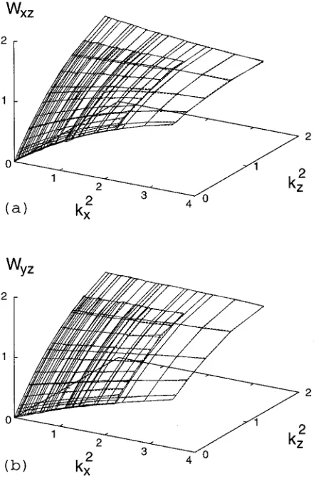
Wxz共k兲⫽

9

具

P2

典

2VkBT

4

具

兩Qxz共k兲兩2

典

⬃ k→0

K11kx2⫹K33kz2, 共30兲

Wy z共k兲⫽

9

具

P2

典

2VkBT

4

具

兩Qy z共k兲兩2

典

⬃

k_→0

K₂₂k_x2_⫹K

33kz2, 共31兲

where the frame is chosen such that k lies in the xz plane关cf. Eqs. 共6兲 and共7兲兴. More specifically, we evaluated the order tensor in Fourier space Q(k) on a k grid with 6⫻6⫻6 grid points in the small system (N⫽4000), and 6⫻6⫻12 grid points in the large system (N⫽16 000). Then we applied a rotation Q(x y z)(k)⫽U(k)Q(XY Z)(k)UT(k) into the desired coordinate frame such that ky⫽0, and calculated the

aver-ages

具

兩Q_␣z(k)兩2

典

and theW␣z(k) surface in that frame.

Be-cause of the constraint on n0, U(k) is a constant throughout

the run.

In the high wavelength limit k→⬁, W_␣z(k) (␣⫽1,2)

takes the value71

W␣z共k兲——→

k→⬁

具

_P

2

典

2␳kBT

具

P2

典

/21⫺4

具

P4

典

/35⫹1/15

. 共32兲

In our simulations, we obtained 1.13, which is in good agree-ment with the theoretical value 1.12.

The results for theW_␣z(k) surfaces are shown in Fig. 1.

The data for the small system 共coarse grid兲 match almost exactly those for the large system 共fine grid兲. They were

fitted to a fourth order polynomial in kx

2

and kz

2 _共

i.e., with highest order terms k_x8,k_x6k_z2,...,k_z8兲 without a zeroth order term. Higher orders were disregarded because the fourth or-der coefficients turned out to be already very small. Normal equations and singular value decomposition gave the same results. Figure 1 demonstrates that the fit is almost perfect. The leading coefficients give the elastic constants, shown in Table I. As expected for elongated molecules, one finds that

K₃₃is largest, followed by K₁₁and K₂₂.

Next we discuss the results for the pair correlation func-tions. The spherical harmonics expansion coefficients of the pair distribution function ␳(2) were determined using84

␳l共₁m₁l₂m₂lm

2兲 _共r兲

⫽4␲%2g共r兲

具

Y_l 1m1

* _共u1兲Yl*₂m₂共u2兲Ylm*共rˆ兲

典

␦r, 共33兲

where

具

•

典

_␦rdenotes the average over all molecules in a shell

␦r from r to r⫹␦r, and the function g(r) is the number of

molecular centers at distance r from a given molecular cen-ter, divided by the number at the same distance in an ideal gas at the same density. The calculation of these averages is very time consuming, since a great number of coefficients has to be evaluated, and was therefore carried out in part on a massively parallel machine. We have determined coeffi-cients for values of l,li up to lmax⫽6 in all systems, and for

values up to lmax⫽8 in the smallest system. The bin size was ␦r⫽0.04 and the cutoff distance rmaxwas chosen to be 40%

of the box side L in order to reduce boundary effects.85 From the pair distribution function we calculated the to-tal correlation function by inverting Eq.共22兲. The latter was then Fourier transformed according to Eq. 共23兲. There is a subtle problem here: due to the elasticity of the nematic phase, the total correlation function decays algebraically like 1/r. This follows directly from Eq.共1兲.3Before applying Eq. 共23兲, we thus fitted the simulation data points at the largest distances r⬎r0to a power law of the form b/r and

extrapo-lated h(r) to infinity.86 The parameter r0 was chosen to be

2.8, 4.0, and 5.3 in systems of N⫽1000, 4000, and 8000 particles, respectively.

It turned out that the long-range tail was quite pro-nounced for coefficients of h with m₁⫽⫾1,m₂⫽⫾1, and almost negligible for the others. In Fig. 2 we show an ex-ample of a coefficient with a pronounced long-range tail, the coefficient h_l

1m1l2m2lm(r) with l1⫽l2⫽l⫽2, m1⫽1, m2

⫽⫺1 and m⫽0. The data for different system sizes N

⫽1000, N⫽4000, and N⫽8000 lie almost on top of each other, hence the form of h(r) at r⬍rmaxis not affected by

FIG. 1. Wxz 共a兲 and Wy z 共b兲 surfaces for N⫽4000 共cubic box兲and N

⫽16 000共elongated box兲; the smaller, finer spaced grids correspond to the larger system. The fits共dotted lines兲coincide almost perfectly with the data 共solid lines兲.

TABLE I. Elastic constants from the analysis of order tensor fluctuations for systems of different size N.

System size

Order tensor fluctuations

具K11典 具K22典 具K33典

4 000 0.53⫾0.01 0.30⫾0.01 1.60⫾0.01

noticeable finite size effects. The dominating finite size prob-lem comes from the uncertainty of the extrapolation, if the available range of h(r) is too short.

The rest of the analysis was straightforward. From the coefficients of the total correlation function in Fourier space,

hl₁m₁l₂m₂lm(k), those of the DCF were obtained by solving

the linear matrix equation共24兲. Then we calculated the func-tions Cii(k) as defined in Eq.共26兲. According to Eq.共25兲, the

elastic constants Kiican be determined from the initial slopes

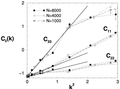
in a plot of Cii(k) versus k2. Data for Cii(k) are shown for

different system sizes in Fig. 3. The points at zero wave vector Cii(0) were calculated using Eq.共27兲. They fit nicely

on the straight lines at k→0, hence the data are consistent with the requirement共14兲or共27兲. This gave additional con-fidence in the quality of the analysis. The slopes of the straight lines yield the elastic constants.

The results are summarized in Table II. We have calcu-lated the DCF from the pair distribution function ␳(2) _using

an upper cutoff l_max⫽2,4, and 6, respectively, in the matrix equations共22兲and共24兲. Already the lowest order calculation with lmax⫽2 gave elastic constants of the correct order of

magnitude. Quantitatively reliable results were obtained with

lmax⭓6: we checked in the smallest system that the results

from calculations with lmax⫽6 and lmax⫽8 do not differ

sig-nificantly.

Since the calculations with lmax⫽8 were very time

con-suming 共one has 1447 different expansion coefficients兲, we used lmax⫽6 in the analyses of the larger systems 共469

dif-ferent expansion coefficients兲.

The results were the same for systems of size N

⫽1000, 4000, and 8000. Furthermore, they were not af-fected by the presence of a director constraint: as mentioned in Sec. III, the DCF was mostly calculated in unconstrained systems, but we also studied the DCF in one constrained system for comparison.

Finally, we compare the values of the elastic constants calculated by the DCF approach with those obtained from the order fluctuation analysis, shown in Table I. The values for K11 and K22 are identical for both methods. K33 is

slightly underestimated by the DCF analysis with lmax⫽6,

but the result increases with l_max, and agrees within the error with that of the order fluctuation analysis at l_max⫽8.

One might ask how much the successive coefficients of the 共correct兲 DCF contribute to the elastic constants. We found that the contribution of the coefficients with l₁⬎4, l₂

⬎4 or l⬎4 is very small. If we include only terms up to

l,li⫽4 in Eq. 共26兲, we obtain K11⫽0.55, K22⫽0.21, and K33⫽1.51 共in the largest system N⫽8000兲, which is very

close to the final values quoted in Table II. However, we could not push this analysis further. If we include only terms up to l,li⫽2, the resulting Cii(k) are very concave and have

no well-defined initial slope in a plot versus k2. Hence the FIG. 2. Expansion coefficient h212– 120(r) of the total correlation function h

vs r in systems of size N⫽8000共solid line兲, N⫽4000共dotted line兲, and

N⫽1000共dashed line兲. Cutoff radii were rmax⫽11.9,9.4, and 6.6, respec-tively. The long dashed line indicates the extrapolation towards r→⬁ 共for the dataset N⫽1000). Inset shows same data vs 1/r.

FIG. 3. Weighted sum of the DCF expansion coefficients Cii(k) as defined

in Eq.共26兲vs k2_{for different system sizes N共unconstrained director,} evalu-ated using coefficients up to lmax⫽6). The points at k⫽0 are taken from Eq.

共27兲. The initial slopes give the elastic constants Kii. Thick solid lines

indicate corresponding fits for the N⫽4000 system.

TABLE II. Elastic constants from the DCF method for systems of different size N. 共*兲 marks a system that has been simulated with a director con-straint. Results are shown for different choices of the cutoff value lmaxin the spherical harmonics expansion of the pair distribution function ␳(2). See Sec. IV for details.

System size

Direct correlation function

lmax 具K11典 具K22典 具K33典

1000 8 0.55⫾0.02 0.35⫾0.03 1.56⫾0.04

6 0.51⫾0.02 0.34⫾0.03 1.52⫾0.04 4 0.53⫾0.03 0.23⫾0.02 1.32⫾0.04 2 0.51⫾0.01 0.20⫾0.01 1.56⫾0.04

4000 6 0.51⫾0.02 0.31⫾0.01 1.51⫾0.03

4 0.65⫾0.02 0.27⫾0.02 1.23⫾0.03 2 0.53⫾0.01 0.22⫾0.01 1.46⫾0.03

*4000 6 0.52⫾0.02 0.31⫾0.01 1.51⫾0.03

4 0.65⫾0.02 0.27⫾0.02 1.24⫾0.04 2 0.53⫾0.01 0.22⫾0.01 1.48⫾0.03

8000 6 0.51⫾0.02 0.33⫾0.02 1.48⫾0.03

contributions of successive ls to the elastic constants cannot be distinguished.

V. SUMMARY AND CONCLUSIONS

We have presented a method which allows one to deter-mine without approximations the direct correlation functions in nematic liquid crystals from computer simulations, and to calculate elastic constants on that basis according to the Poniewierski–Stecki theory35 共2兲–共4兲. We have applied this method to a nematic fluid of soft ellipsoids. In the same system, the elastic constants were also determined by an es-tablished approach, the analysis of order tensor fluctuations. Our study represents a direct test of the Poniewierski– Stecki theory. We found that the results obtained with the two methods agree well with each other. The Poniewierski– Stecki theory can thus be employed to calculate elastic con-stants, at least in our system, provided that the exact direct correlation functions are used in the equations.

Hence we have established an alternative way of calcu-lating elastic constants in nematic liquid crystals. As long as a simulation is performed solely to determine elastic con-stants, the order tensor fluctuation approach is still more ef-ficient: the statistical error of pair correlation functions must be quite small for a reliable DCF analysis, and the analysis is very time consuming. However, the DCF approach has the advantage of being straightforward; elastic constants can be computed from arbitrary bulk simulations, if the pair distri-bution functions are known with sufficient accuracy. Even the calculation of spatially varying elastic constants, e.g., in the vicinity of surfaces, is conceivable.

The direct correlation function is a central quantity in liquid state theories. The study of direct correlation functions in the nematic phase is therefore interesting in its own right. We shall examine them in more detail and compare them to those in the isotropic phase in a forthcoming publication.87

ACKNOWLEDGMENTS

The authors thank M. P. Allen and H. Lange for fruitful interactions, and P. Teixeira for helpful comments on the paper. The simulations and the analyses were run in part on a CRAY T3E of the HLRZ in Ju¨lich. Two of the authors 共N.H.P. and G.G.兲 received financial support from the Ger-man Science Foundation 共DFG兲. The parallel MD program GBMEGA used in this work was originally developed by the EPSRC Complex Fluids Consortium, UK.

1_{P.-G. de Gennes and J. Prost, The Physics of Liquid Crystals 共Oxford} University Press, Oxford, 1995兲.

2_{S. Chandrasekhar, Liquid Crystals共Cambridge University Press,} Cam-bridge, 1992兲.

3_{D. Forster, Hydrodynamic fluctuations, broken symmetry and correlation} functions, Frontiers in Physics共Benjamin, Reading, MA, 1975兲, Vol. 47. 4_{P. M. Chaikin and T. C. Lubensky, Principles of Condensed Matter}

Phys-ics共Cambridge University Press, Cambridge, 1995兲. 5

C. Oseen, Trans. Faraday Soc. 29, 883共1933兲; H. Zo¨cher, ibid. 29, 945

共1933兲.

6_{F. C. Frank, Discuss. Faraday Soc. 25, 19共1958兲.} 7_{T. C. Lubensky, Phys. Lett. A 33, 202共1970兲.} 8

J. Nehring and A. Saupe, J. Chem. Phys. 54, 337共1971兲; 54, 337共1971兲. 9_{R. G. Priest, Mol. Cryst. Liq. Cryst. 17, 129共1972兲; Phys. Rev. A 7, 720}

共1973兲.

10_{J. P. Straley, Phys. Rev. A 8, 2181共1973兲.} 11_{T. E. Faber, Proc. R. Soc. London 353, 261共1977兲.}

12_{D. A. Dunmur and W. H. Miller, Chem. Phys. Lett. 86, 353共1982兲.} 13_{Th. W. Ruijgrok and K. Sokalski, Physica A 111, 45共1982兲.} 14

B. W. Van Der Meer, F. Postma, A. J. Dekker, and W. H. De Jeu, Mol. Phys. 45, 1227共1982兲.

15_{W. M. Gelbart and A. Ben-Shaul, J. Chem. Phys. 77, 916共1982兲.} 16_{S. Sarkar and R. J. A. Tough, J. Phys. I 43, 1543共1982兲.}

17_{G. Vertogen, S. D. P. Flapper, and C. Dullemond, J. Chem. Phys. 76, 616}

共1982兲.

18_{G. Vertogen, Phys. Lett. A 89, 448共1982兲.}

19_{E. Govers and G. Vertogen, Liq. Cryst. 2, 31共1987兲.} 20

E. Govers and G. Vertogen, Physica A 150, 1共1988兲. 21_{E. Govers and G. Vertogen, Liq. Cryst. 5, 323共1989兲.}

22_{B. Tjipto-Margo and D. E. Sullivan, J. Chem. Phys. 88, 6620共1988兲.} 23

S.-W. Lo and R. A. Pelcovits, Phys. Rev. E 42, 4756共1990兲. 24_{G. Marrucci and F. Greco, Mol. Cryst. Liq. Cryst. 206, 17共1991兲.} 25_{A. V. Zakharov, Physica A 175, 327共1991兲.}

26_{A. V. Zakharov and S. Romano, Phys. Rev. E 58, 7428共1998兲.} 27_{A. V. Zakharov and R. J. Dong, Phys. Rev. E 630, 1704共2001兲.} 28

R. G. Petschek and E. M. Terentjev, Phys. Rev. E 45, 930共1992兲. 29_{M. A. Osipov and S. Hess, Mol. Phys. 78, 1191共1993兲.} 30_{M. A. Osipov and S. Hess, Liq. Cryst. 16, 845共1994兲.} 31

L. R. Evangelista, I. Hibler, and A. J. Palangana, Nuovo Cimento D 18, 33

共1996兲.

32_{L. R. Evangelista, I. Hibler, and H. Mukai, Phys. Rev. E 58, 3245共1998兲.} 33

P. A. de Castro, A. J. Palangana, and L. R. Evangelista, Phys. Rev. E 60, 6195共1999兲.

34

T. Sato and A. Teramoto, Macromolecules 29, 4107共1996兲. 35_{A. Poniewierski and J. Stecki, Mol. Phys. 38, 1931共1979兲.} 36_{A. Poniewierski and J. Stecki, Phys. Rev. A 25, 2368共1982兲.} 37

Y. Singh, Phys. Rev. A 30, 583共1984兲; Liq. Cryst. 2, 31共1987兲. 38_{Y. Singh and K. Singh, Phys. Rev. A 33, 3481共1986兲.} 39_{Y. Singh, S. Singh, and K. Rajesh, Phys. Rev. E 45, 974共1992兲.} 40

S. Singh, Phys. Rep. 277, 284共1996兲.

41_{M. D. Lipkin, S. A. Rice, and U. Mohanty, J. Chem. Phys. 82, 472共1985兲.} 42_{P. I. C. Teixeira, V. M. Pergamenshchik, and T. J. Sluckin, Mol. Phys. 80,}

1339共1993兲.

43_{A. M. Somoza and P. Tarazona, Mol. Phys. 72, 911共1991兲.} 44

H. Yokoyama, Phys. Rev. E 55, 2938共1997兲. 45_{A. Kapanowski, Phys. Rev. E 55, 7090共1997兲.}

46_{L. Longa, J. Stelzer, and D. Dunmur, J. Chem. Phys. 109, 1555共1998兲.} 47

J. Stecki and A. Poniewierski, Mol. Phys. 41, 1451共1980兲. 48_{A. Poniewierski and R. Holyst, Phys. Rev. E 41, 6871共1990兲.} 49_{V. P. Veshnev and I. I. Ptichkin, Kristallografiya 34, 1217共1989兲.} 50

K. Singh and Y. Singh, Phys. Rev. A 34, 548共1986兲; 35, 3535共1987兲. 51_{J. Ram and Y. Singh, Phys. Rev. E 44, 3718共1991兲.}

52

S. Singh, Liq. Cryst. 20, 797共1996兲.

53_{T. K. Lahiri, K. Rajesh, and S. Singh, Liq. Cryst. 22, 575共1997兲.} 54_{K. Singh and N. S. Pandey, Liq. Cryst. 25, 411共1998兲.}

55

A. M. Somoza and T. Tarazona, Phys. Rev. A 40, 6069共1989兲. 56_{B. Tjipto-Margo, G. T. Evans, M. P. Allen, and D. Frenkel, J. Phys. Chem.}

96, 3942共1992兲. 57

Z. D. Zhang and G. C. Yang, J. Mater. Sci. Technol. 15, 377共1999兲. 58_{M. F. Holovko and T. G. Sokolovska, J. Mol. Liq. 82, 161共1999兲.} 59_{R. Evans, in Fundamentals of Inhomogeneous Fluids, edited by D.}

Henderson共Marcel Dekker, New York, 1992兲, p. 86.

60_{J. P. Hansen and I. R. McDonald, Theory of Simple Liquids共Academic,} London, 1986兲.

61_{C. G. Gray and K. E. Gubbins, Theory of Molecular Fluids共Oxford} Uni-versity Press, Oxford, 1984兲, Vol. 1.

62

J. Stelzer, L. Longa, and H. R. Trebin, J. Chem. Phys. 103, 3098共1995兲;

107, 1295共1997兲.

63_{J. Stelzer, L. Longa, and H. R. Trebin, Mol. Cryst. Liq. Cryst. 262, 455}

共1995兲.

64_{J. Stelzer, M. A. Bates, L. Longa, and G. R. Luckhurst, J. Chem. Phys.}

107, 7483共1997兲.

65_{A. V. Zakharov and A. Maliniak, Eur. Phys. J. E 4, 85共2001兲.}

67_{L. Longa, G. Cholewiak, R. Trebin, and G. R. Luckhurst, Eur. Phys. J. E}

4, 51共2001兲.

68_{M. P. Allen and D. Frenkel, Phys. Rev. A 37, 1813 共1988兲; 42, 3641}

共1990兲.

69_{M. P. Allen and D. J. Cleaver, Phys. Rev. E 43, 1918共1991兲.} 70_{M. P. Allen and A. J. Masters, Mol. Phys. 79, 277共1993兲.}

71_{M. P. Allen, M. A. Warren, M. R. Wilson, A. Sauron, and W. Smith, J.} Chem. Phys. 105, 2850共1996兲.

72

C. Zannoni, in Advances in the Computer Simulations of Liquid Crystals, NATO Science Series C Vol. 545, edited by P. Pasini and C. Zannoni

共Kluwer Academics, Dordrecht, 2000兲, p. 17. 73_{K. E. Gubbins, Chem. Phys. Lett. 76, 329共1980兲.} 74

B. J. Berne and P. Pechukas, J. Chem. Phys. 56, 4213共1975兲. 75

The pressure was determined from the simulation data. The temperature was a fixed parameter in the Monte Carlo simulations. The molecular dynamics simulations were carried out in the microcanonical ensemble with the total energy adjusted such that the temperature had the desired value. Statistical errors are in the third decimal place.

76_{H. Lange, Ph.D. thesis, Universita¨t Mainz共2001兲.}

77_{H. C. Andersen, J. Comput. Phys. 52, 24共1983兲.} 78

M. P. Allen and D. J. Tildesley, Computer Simulations of Liquids共Oxford University Press, Oxford, 1989兲.

79_{In our scaling, the time unit is}冑_m 0/⑀0␴0. 80_{G. Germano共in preparation兲.}

81_{G. Germano and M. P. Allen共in preparation兲.} 82

J. G. Gay and B. J. Berne, J. Chem. Phys. 74, 3316共1981兲. 83_{The choice of an elongated box was motivated by the fact that K}

33is about twice as large as K11and K22. Equations共6兲,共7兲or共30兲,共31兲reveal that it is of advantage to work on a k-grid, which is finer in the z direction than in the other two.

84_{W. B. Streett and D. J. Tildesley, Proc. R. Soc. London, Ser. A 348, 485}

共1975兲.

85_{L. R. Pratt and S. W. Haan, J. Chem. Phys. 74, 1873共1980兲.} 86

For a few coefficients, it was also necessary to shift the data by a constant. See Ref. 87 for a more detailed presentation of the data analysis. 87