ABSTRACT
SHEN, SHITIAN. Improving Learning & Reducing Time: A Constrained Action Based Reinforcement Learning Approach. (Under the direction of Min Chi.)
Intelligent Tutoring Systems (ITSs) have been shown to be highly effective at improving student learning in real classrooms through scaffolding, adaptive supports and contextualized feedback to individual learners. ITSs generally need to decidewhat to teach such as which problem is assigned to students andhow to teach such as whether present a problem as a problem solving or a worked example, with the guide ofpedagogical strategy, which maps students’ behavior information and current learning context into an optimal decision. However, inducing an effective pedagogical strat-egy (policy) is challenging due to the lack of learning theory for decision-making in the ITSs and modeling for the relation between the pedagogical decision and student learning. There is a clear need to advance data-driven approaches to address this challenge.
Specifically, we applied the data-driven approaches to deal with a particular type of pedagogi-cal decision: problem solving (PS) vs. worked example (WE) in an ITS named Deep Thought, which teaches undergraduate students logic proof and strictly controls the learning content to be equiv-alent to individual students. When solving a PS, students are required to complete a problem with tutor’s support such as hint, while students are provided with a problem as well as an expert solu-tion step by step when doing a WE. In this work, we construct the effective pedagogical strategy in an offline manner using three different Reinforcement Learning (RL) frameworks including tabu-lar Markov Decision Process (MDP), Partially Observable MDP (POMDP), and constrained action-based POMDP (CAPOMDP).
We explored four aspects of the RL framework: 1) state representation: presenting students’ learning behavior and learning context based on either the set of selected features or the belief state space where each state is associated with the probability; 2)reward function: investigating the impact of immediate and delayed rewards on the effectiveness of policies, and detecting the ef-fectiveness of policies using learning gain and time as reward separately; 3)policy execution: com-paring the effectiveness of stochastic policy execution with that of the deterministic execution; 4) action-based constraints: investigate the impact of constraints on the effectiveness of policies.
© Copyright 2019 by Shitian Shen
Improving Learning & Reducing Time: A Constrained Action Based Reinforcement Learning Approach
by Shitian Shen
A dissertation submitted to the Graduate Faculty of North Carolina State University
in partial fulfillment of the requirements for the Degree of
Doctor of Philosophy
Computer Science
Raleigh, North Carolina
2019
APPROVED BY:
Tiffany Barnes Jonathan Rowe
Dennis Bahler Min Chi
ACKNOWLEDGEMENTS
TABLE OF CONTENTS
LIST OF TABLES . . . vi
LIST OF FIGURES. . . .viii
Chapter 1 Introduction. . . 1
1.1 Pedagogical Decision: Worked Example vs. Problem Solving . . . 2
1.2 Reinforcement Learning Frameworks . . . 2
1.2.1 Tabular MDP Framework . . . 3
1.2.2 POMDP Framework . . . 3
1.2.3 CAPOMDP Framework . . . 4
1.3 Contributions . . . 4
1.4 Outline of the Thesis . . . 6
Chapter 2 Related Work . . . 7
2.1 Pedagogical Decisions: Worked Example vs. Problem Solving . . . 7
2.2 Applying RL into Educational Domain . . . 9
2.2.1 Markov Decision Process (MDP) . . . 9
2.2.2 Partially Observable Markov Decision Process (POMDP) . . . 10
2.2.3 Deep RL Framework . . . 10
2.2.4 Summarization of RL Applications in Educational Domain . . . 11
2.3 Constrained Reinforcement Learning . . . 11
2.4 Aptitude Treatment Interaction Effect . . . 12
Chapter 3 Markov Decision Process . . . 14
3.1 Introduction . . . 14
3.2 MDP Framework . . . 15
3.2.1 Policy Induction . . . 16
3.2.2 Policy Evaluation . . . 16
3.2.3 Stochastic Policy Execution . . . 17
3.3 Pedagogical Decisions in a Logic Tutor: Deep Thought . . . 18
3.3.1 Overview of Deep Thought . . . 18
3.3.2 Two Training Datasets:DT-Imme and DT-Delay . . . 20
3.3.3 Feature Set . . . 20
3.4 Feature Selection on the MDP Framework . . . 21
3.4.1 Related Work For Feature Selection in RL . . . 22
3.4.2 Five Correlation Metrics . . . 22
3.4.3 Correlation-based Feature Selection Approaches . . . 24
3.4.4 PreRL-FS Approach . . . 25
3.4.5 Ensemble Approach . . . 26
3.4.6 Comparison Results for Feature Selection Approaches . . . 26
3.5 Experiments Overview . . . 28
3.5.1 Research Questions . . . 28
3.5.3 Experiments Overview . . . 29
3.5.4 ATI effect: Splitting Students Based on Response Time . . . 30
3.5.5 Statistic Analysis . . . 31
3.6 Four Experiments . . . 31
3.6.1 Experiment 1: Preliminary Feature Selection . . . 31
3.6.2 Experiment 2: Ensemble Feature Selection & Immediate vs. Delayed Rewards 34 3.6.3 Experiment 3: Low Correlation-based Feature Selection . . . 38
3.6.4 Experiment 4: Stochastic Policy Execution . . . 41
3.6.5 Conclusions of Experiments . . . 42
3.7 Post-hoc Comparisons . . . 43
3.7.1 Global Median Split . . . 44
3.7.2 The Impact of Feature Selection on RL Policies . . . 45
3.7.3 Problem Solving vs. Worked Example under policies . . . 47
3.8 Conclusions, Limitations, & Discussion . . . 49
Chapter 4 Partially Observable Markov Decision Process . . . 52
4.1 Introduction . . . 52
4.2 POMDP Framework . . . 53
4.2.1 Feature Transformation . . . 54
4.2.2 Belief State Estimation . . . 54
4.2.3 POMDP Policy Induction . . . 55
4.3 Experiments Overview & Research Questions . . . 55
4.3.1 Induced Policies . . . 55
4.3.2 Research Questions . . . 56
4.3.3 Empirical Evaluation . . . 56
4.4 Experiment 1: POMDP with Selected Features . . . 57
4.4.1 Participants & Conditions . . . 57
4.4.2 Results . . . 57
4.4.3 Conclusion & Discussion . . . 58
4.5 Experiment 2: POMDP with a wide range of features . . . 58
4.5.1 Participants & Conditions . . . 58
4.5.2 Results . . . 58
4.5.3 Conclusion & Discussion . . . 60
4.6 Post-hoc Comparison . . . 60
4.6.1 Across Six Groups . . . 60
4.6.2 POMDP vs. MDP Framework . . . 62
4.6.3 Stochastic vs. Deterministic Policy Execution . . . 62
4.6.4 Post-hoc Discussion . . . 64
4.7 Conclusions, Limitations, & Discussion . . . 64
Chapter 5 Constrained Action-based POMDP . . . 65
5.1 Introduction . . . 65
5.2 Problem Statement . . . 67
5.3 Constrained Action-based POMDP (CAPOMDP) . . . 68
5.3.2 Reward Function . . . 69
5.3.3 Policy Induction . . . 70
5.4 Experiment Setup . . . 70
5.4.1 Procedure & Evaluation . . . 70
5.4.2 Training Corpus . . . 71
5.4.3 Policy Execution . . . 72
5.5 Experiment Overview & Research Questions . . . 72
5.5.1 Induced Policies . . . 72
5.5.2 Research Questions . . . 73
5.6 Experiment 1: Improving Learning Gain Using CAPOMDP . . . 74
5.6.1 Participants & Conditions . . . 74
5.6.2 Experiment 1 Results . . . 75
5.6.3 Experiment 1 Conclusion . . . 78
5.7 Experiment 2: Reducing Total Time Using CAPOMDP . . . 78
5.7.1 Participants & Conditions . . . 78
5.7.2 Experiment 2 Result . . . 79
5.7.3 Experiment 2 Conclusion . . . 82
5.8 Post-hoc Comparisons . . . 83
5.8.1 Participants & Conditions . . . 83
5.8.2 Post-hoc Comparison Results . . . 84
5.8.3 Conclusion of Post-hoc Comparisons . . . 88
5.9 Log Analysis . . . 88
5.9.1 Impact of Action-based Constraints on Learning Performance . . . 88
5.9.2 Relation between Behaviors to Learning Outcomes . . . 90
5.9.3 Impact of Pedagogical Strategy on Behavior . . . 93
5.9.4 Summarization of Log Analysis . . . 97
5.10 Conclusion & Discussion . . . 97
Chapter 6 Conclusions and Future Work. . . 99
6.1 Conclusions . . . 99
6.2 Limitation . . . 100
6.3 Future Work . . . 101
LIST OF TABLES
Table 2.1 Reinforcement Learning Applications in Educational Domain . . . 11
Table 3.1 Reinforcement Learning Policies in Four Experiments . . . 29
Table 3.2 Overview of Experiments . . . 30
Table 3.3 MDP-ECRPolicy . . . 32
Table 3.4 Pre-test and Transfer Post-test in Experiment 1 . . . 33
Table 3.5 Ensemble-Imme Policy . . . 35
Table 3.6 Ensemble-Delay Policy . . . 36
Table 3.7 Pre-test and Transfer Post-test in Experiment 2 . . . 37
Table 3.8 Pairwise Contrasts on Adjusted Transfer Post-test in Experiment 2 . . . 38
Table 3.9 WIG-Low Policy . . . 39
Table 3.10 Pre-test and Transfer Post-test in Experiment 3 . . . 40
Table 3.11 Pre-test and Transfer Post-test in Experiment 4 . . . 42
Table 3.12 Size of each group in post-hoc comparisons . . . 44
Table 3.13 Pre-test and Transfer Post-test Score across Experiment 1-3 . . . 45
Table 3.14 Pairwise Contrasts on Adjusted Transfer Post-test in Post-hoc Comparison . . . 46
Table 3.15 PS and WE Counts and Comparisons for each Policy across Experiment 1-3 . . 48
Table 4.1 Implemented policies in two experiments for POMDP study . . . 55
Table 4.2 Overview of Experiments . . . 56
Table 4.3 Mean and SD of learning performance for each condition in Experiment 1 . . . 57
Table 4.4 Mean and SD of Behavior Variables for each condition in Experiment 1 . . . 58
Table 4.5 Mean and SD of learning performance for each condition in Experiment 2 . . . 59
Table 4.6 Mean and SD of behavior variables for each condition in Experiment 2 . . . 59
Table 4.7 learning Performance In Post-hoc comparison For POMDP Study . . . 61
Table 4.8 Learning performance for each framework in post-hoc comparison . . . 63
Table 4.9 Learning performance for each policy execution in post-hoc comparison . . . . 63
Table 5.1 Implemented policies in two experiments for CAPOMDP study . . . 73
Table 5.2 Overview of Experiments . . . 74
Table 5.3 Participants and Conditions in Experiment 1 . . . 75
Table 5.4 Learning Performance in Experiment 1 . . . 76
Table 5.5 Learning Performance of HighIC Groups in Experiment 1 . . . 77
Table 5.6 Learning Performance of LowIC Groups in Experiment 1 . . . 77
Table 5.7 Participants and Conditions in Experiment 2 . . . 79
Table 5.8 Learning Performance in Experiment 2 . . . 80
Table 5.9 Learning Performance of HighIC Groups by condition in Experiment 2 . . . 81
Table 5.10 Learning Performance of LowIC Groups by condition in Experiment 2 . . . 81
Table 5.11 Participants and Conditions in Post-hoc Comparison . . . 83
Table 5.12 Learning Performance in Post-Hoc Comparison . . . 84
Table 5.13 Learning Performance of HighIC Groups in Post-Hoc Comparison . . . 85
Table 5.14 Learning Performance of LowIC Groups in Post-Hoc Comparison . . . 85
LIST OF FIGURES
Figure 3.1 Interface for Worked Example . . . 18
Figure 3.2 Interface for Problem Solving . . . 19
Figure 3.3 DT-Immed . . . 26
Figure 3.4 DT-Delay . . . 26
Figure 3.5 DT-Immed . . . 27
Figure 3.6 DT-Delay . . . 27
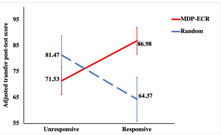
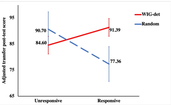
Figure 3.7 Interaction effect for the adjusted transfer post-test score in Experiment 1 . . 33
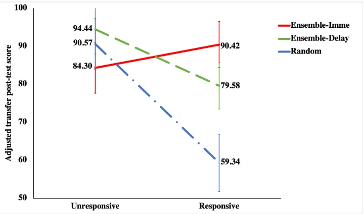
Figure 3.8 Interaction effect for the adjusted transfer post-test score in Experiment 2 . . 37
Figure 3.9 Interaction effect for the adjusted transfer post-test score in Experiment 3 . . 40
Figure 3.10 Interaction effect for adjusted transfer post-test score across Experiment 1-3 . 46 Figure 4.1 The process of POMDP policy induction . . . 54
Figure 5.1 The general process of the CAPOMDP policy induction . . . 68
Figure 5.2 Unconstrained policy execution . . . 72
CHAPTER
1
INTRODUCTION
Intelligent Tutoring Systems (ITSs), as one type of highly interactive e-learning environment, have been widely used in the educational domain[D’M11; Koe97; Van07]. While ITSs hold great promise, they are difficult and expensive to construct and are often brittle and inflexible in their interactions with students. The effective ITSs generally provide step-by-step adaptive support and contextual-ized feedback to individual learners at run-time[Koe97; Van06], and determinewhat to teach such as which problem is present to students, andhow to teach such as whether give a hint, whether present a given problem as a worked example. The step-by-step behavior can be viewed as a se-quential decision process where at each step the system chooses an appropriate action from a set of options. This decision process is governed by thepedagogical strategy or policy which selects the action based upon the given user input and the current learning context[Igl09b].
is a clear need to advance data-driven approaches for pedagogical decision-making.
1.1
Pedagogical Decision: Worked Example vs. Problem Solving
In this work, we induce the pedagogical strategy in an ITS, called Deep Thought (DT)[MB17], which teaches undergraduate students logic proof in “Discrete Mathematics” course at NCSU. DT con-tains a total of seven learning phases or levels covering different knowledge components. Our goal is to induce an effective policy to deal with a particular type of pedagogical decision in DT: whether to provide students with aWorked Example (WE)of a problem or to ask them to engage inProblem Solving (PS). When providing a WE, the tutor will show an expert solution to a problem step by step, while students are required to complete a problem independently with tutor’s support such as hint when solving a PS. Since students are required to solve the same set of problems either in PS or WE, the contents of DT are strictly controlled to be equivalent, which makes the pedagogical strategy induction task more challenging. One possible reason is that there is limited space for the peda-gogical strategy to improve students’ learning performance comparing with the baseline strategy. Although there are many different theories about when and how to provide WE or PS, widespread consensus does not exist. This is why we chose to take a data-driven approach to induce the policy. More importantly, little evidence has been presented to date demonstrating that ITSs have effec-tive pedagogical skills or that their pedagogical decisions have a direct impact on student learning when the content is controlled to be equivalent.
1.2
Reinforcement Learning Frameworks
1.2.1 Tabular MDP Framework
We explore the tabular MDP framework from three aspects including 1) thereward function: in-duce policies using either immediate or delayed reward; 2) thestate representation: propose the correlation-based feature selection approaches to construct various discrete state space based on different set of discretized features for policy induction; and 3)policy execution: execute the policy deterministically or stochastically on the run time of tutor.
We conduct four experiments from Spring 2015 to Fall 2016 in order to answer three research questions based on the tabular MDP framework: 1) Does the immediate reward facilitate the MDP framework to induce a more effective pedagogical policy than the delayed reward ? 2) Does the correlation-based feature selection approach have a positive impact on the effectiveness of the policy ? 3) Can stochastic policy execution further improve the effectiveness of the induced policy as compared to deterministic execution?
We note that the tabular MDP framework has two weaknesses. First, tabular MDPs are not able to efficiently deal with high dimensional feature spaces including both discrete and continuous variables. In particular, there is no prior knowledge about the appropriate structure of state rep-resentations for learning pedagogical policies in the ITS domain. Although we implement a fea-ture selection approach to construct the state space, we can’t guarantee that the state space and the transitions among states are able to fully express students’ learning behaviors and learning process, respectively. Second and more important, many other factors such as motivation, affect, prior knowledge and proficiency, are useful for decision-making, but they can neither be observed directly nor described explicitly, and thus cannot be included in the MDP framework.
1.2.2 POMDP Framework
Different from tabular MDP, POMDP generates a belief state space, which comprises probabil-ity distributions over latent states. Specifically, POMDP assigns probabilprobabil-ity to each latent state given the observation with a wide range of features at each time step[Pin03; Pin06]. Consequently, POMDP is able to deal with a large set of features, which can be efficiently transferred into a belief state space. Although the belief state is hard to interpret, prior research has verified that it is useful to track students’ mastery of Knowledge Components[Cle16]and knowledge level[Man14; Raf16]. Therefore, we hypothesize that the POMDP framework can induce an effective policy.
also explore the POMDP policy execution: deterministic vs. stochastic. Specifically, we have three research questions: 1) Does POMDP induce more effective policy than MDP and Random given a limited feature set ? 2) Is the POMDP policy, induced given a wide range of features, more effective than the MDP and Random policies ? 3) Can stochastic POMDP policy execution further improve the effectiveness of the POMDP policy as compared to deterministic execution?
1.2.3 CAPOMDP Framework
It is worthwhile to mention that both POMDP and MDP frameworks are used to handle the stan-dard RL scenario and to induce the unconstrained policies. Different from POMDP and MDP, we construct the constrained based POMDP (CAPOMDP) framework by integrating the action-based constraints into the POMDP framework, to deal with aconstrained action-based RL (CARL) scenario, which involves the additional action-based constraints such as a maximum number of times that an agent may take a specific action. For instance, the action-based constraints in DT are presented as: the last problem on each level must be done in PS, and prior to reaching that problem the students must complete at least one PS and one WE. DT did not allow students stay in the extreme situation where they always solve PS or WE in a level. In this scenario, the early deci-sions impose special constraints on the future actions. In other words, the available actions for an agent at any given situation are governed not only by the current state but also by prior decisions. Consequently, when deciding the next action, the agent should take these constraints into account. Therefore, we apply CAPOMDP to induce the constrained policy.
Furthermore, we induce two types of constrained policies:CAPOMDPLG using learning gain as the immediate reward for improving students’ learning performance, andCAPOMDPTime us-ing time as the immediate reward for reducus-ing students’ time on task. We conduct two empiri-cal studies from Fall 2017 to Spring 2018 for comparing the effectiveness ofC AP O M D PLG and C AP O M D PLG with three baselines including the POMDP policy induced by the full power of POMDP as mentioned above, a Deep Reinforcement Learning induced policy and the random pol-icy. There are three research questions: 1) canCAPOMDPLG outperform baseline policies in terms of learning gain? 2) canCAPOMDPTime significantly reduce students’ time compared with the base-line? 3) Do action-based constraints hurt the effectiveness of unconstrained policies?
1.3
Contributions
contributions are summarized as follows:
• We find that a consistent Aptitude Treatment Interaction (ATI) effect[CS77a; Sno91]exists across studies: certain students are less sensitive to the induced policies in that they achieve a similar learning performance regardless of policies employed, whereas other students are more sensitive in that their learning is highly dependant on the effectiveness of the policies.
• We induce MDP policies based on immediate and delayed rewards respectively and detect that immediate reward facilitates tabular MDP to induce a more effective policy than delayed one through empirical experiments.
• We propose correlation-based feature selection approaches for state representation in the tabular MDP framework, and empirically verify that MDP policies outperform a random baseline in terms of students’ learning performance.
• While previous research mainly execute the RL-induced policies deterministically, we ex-plore both deterministic and stochastic policy execution, and empirical results suggest that the stochastic can be more effective than deterministic execution for both tabular MDP and POMDP policies.
• As of the time of our work on this subject, this is the first study to compare and empirically evaluate the effectiveness of POMDP vs. tabular MDP policies.
• We propose the CAPOMDP framework, a constrained action-based reinforcement learning framework, to induce the policy considering the action-based constraints in our tutor.
1.4
Outline of the Thesis
The rest of the thesis is organized as follows:
Chapter 2: This chapter presents related work required to comprehend the rest of the thesis.
Chapter 3: This chapter presents the application of the MDP framework for pedagogical strategy induction. The MDP policies are constructed based on the set of features selected through different feature selection approaches. Four experiments are conducted to investigate the effectiveness of the MDP policies.
Chapter 4: This chapter shows the application of the POMDP framework. Two empirical studies are conducted to compare the effectiveness of the POMDP policies with that of the MDP and the Random policies.
Chapter 5: In this chapter, the CAPOMDP framework is proposed to deal with the constrained action-based RL problem. The CAPOMDP policies are induced using either learning gain or time as reward. Two empirical studies are conducted to compare the effectiveness of the CAPOMDP policies against the POMDP, Deep RL and the Random policies.
CHAPTER
2
RELATED WORK
2.1
Pedagogical Decisions: Worked Example vs. Problem Solving
A great deal of research has investigated the impacts of worked examples (WE) and problem solving (PS) on student learning[MI11; McL14; Naj14; Sal10]. During PS, students are given a training prob-lem which they must solve independently or with partial assistance, while during WE, students are shown a detailed solution to the problem.
In 2008, McLaren et al.[McL08]compared WE-PS pairs with PS-only, where every student was given the same 10 training problems. Students in the PS-only condition were required to solve every problem while students in the WE-PS condition were given 5 example-problem pairs. Each pair consists of an initial worked example problem followed by tutored problem solving. They found no significant difference in learning performance between the two conditions; however, the WE-PS group spent significantly less time on task than the WE-PS group.
con-dition were givenincorrect worked examples containing between 1 and 4 errors and were tasked with correcting them. Again the authors found no significant differences among the conditions in terms of learning gains, and as before the WE students spent significantly less time than the other groups. More specifically, for time on task they found that:WE<EE<untutored PS<tutored PS. WE students took only 30% of the total time of the tutored PS students.
The advantages of WE were also demonstrated in another study in the domain of electrical circuits[VG11]. In that study, Van et al. compared four conditions: WE, WE-PS pairs, PS-WE pairs (problem-solving followed by an example problem), and PS only. Their results showed that the WE and WE-PS students significantly outperformed the other two groups, and no significant differ-ence was found among four conditions in terms of time on task. Additionally, Razzaq et al.[RH09] designed an experiment on comparing worked examples vs. problem solving in an ITS that teaches mathematics. They found that more proficient students benefit more from WE when controlling for time, while less proficient students benefit more from PS.
Some existing theories of learning suggest that when deciding whether to present PS or WE, a tutor should take into account several factors, including the students’ current knowledge model. Vygotsky[Vyg78]coined the term “zone of proximal development” (ZPD) to describe the space be-tween abilities that a student may display independently and those that they may display with sup-port. He hypothesized that the most learning occurs when students are assigned tasks within their ZPD. In other words, the task should neither be so simple that they can achieve it independently or trivially, nor so difficult that they simply cannot make progress even with assistance. We expect, based upon this theory, that if students are somewhat competent in all the knowledge needed for solving a problem, the tutor should present the problem as a PS, and provide help only if the stu-dents fail so that they can practice their knowledge. If stustu-dents are completely unfamiliar with the problem, however, then the tutor should present the problem as a WE. Brown et al.[Bro89]describe a progression from WE to PS following their “model, scaffold & fade” rubric.[KA07]by contrast de-fined an “assistance dimension”, which includes PSs and WEs. The level of assistance a tutor should provide may be resolved differently for different students and should be adaptive to the learning environment, the domain materials used, the students’ knowledge level, their affect state and so on. Typically, these theories are considerably more general than the specific decisions that ITS de-signers must make, which makes it difficult to tell if a specific pedagogical strategy is consistent with the theory. This is why we wish to derive pedagogical policy for PS/WE directly from empirical data.
Ren02; MI11; Mos15]. As opposed to previous work, which involves hard-coded rules for provid-ing PS or WE, we apply the Reinforcement Learnprovid-ing approach to induce the pedagogical strategy which explicitly indicates how to make decisions given the current state related to students’ learn-ing process, the learnlearn-ing context in the tutor, as well as the predefined constraints.
2.2
Applying RL into Educational Domain
2.2.1 Markov Decision Process (MDP)
MDP[Lit94; SB98a]is a widely used reinforcement learning framework in educational applications. Beck et al.[Bec00]investigated temporal difference learning to induce pedagogical policies that would minimize the time students spend on completing problems in AnimalWatch, an ITS that teaches arithmetic to grade school students. They used simulated students in the training phase of their study and used time as an immediate reward given that student’s time can be assessed at each step. In the test phase, the new AnimalWatch with induced pedagogical policy was empirically compared with the original version. They found that the policy group spent significantly less time per problem than their non-policy peers.
Iglesias and her colleagues applied online Q-learning with time as the immediate reward to generate a policy in RLATES, an intelligent educational system that teaches students database de-sign[Igl09b; Igl09a; Igl03]. The goal of inducing the policy was to provide students with direct nav-igation support through the system’s content and to help them learn more efficiently. They also used simulated students in the training phase and evaluated the induced policy by comparing the performance of both simulated and real students using RLATES with that of other students using IGNATES, which provides indirect navigation support without RL. Their results showed that stu-dents using RLATES spent significantly less time than stustu-dents using IGNATES, but there was no significant difference in students’ level of knowledge, evaluated by the exam.
Martin et al.[MA04]applied a model-based RL method with delayed reward to induce policies that would increase the efficiency of hint sequencing on Wayang Outpost, a web-based ITS which prepares students for the mathematics section of the Scholastic Aptitude Test. During the training phase, the authors used a student model to generate the training data for inducing the policies. In the test phase, the induced RL policies were tested on a simulated student model and students’ performance was evaluated by learning level, a customized score function. The results showed that simulated students following RL policies achieved a significantly better learning level than the non-policy group.
train-ing human students on the ITS that makes random decisions. Their empirical evaluation showed the induced policies were significantly more effective than the previous policies based on students’ normalized learning gain (NLG).
2.2.2 Partially Observable Markov Decision Process (POMDP)
POMDP[Jaa95; KS98]is another widely used framework in educational domains. Different from the MDP framework where the state space is constructed by a set of observable features, the POMDP framework uses a belief state space to model the unobserved factors, such as students’ knowledge level and proficiency. Mandel et al.[Man14]combined a feature compression approach that can handle a large range of state features with POMDP to induce policies for an educational game. The induced policies with the immediate reward outperformed both random and expert-designed poli-cies in both simulated and empirical evaluations.
Rafferty et al.[Raf16]applied POMDP to represent students’ latent knowledge by combining embedded graphical models for concept learning with interpreted belief states in the domain of alphabet arithmetic. They applied POMDP to induce policies using time as the reward, with a goal of reducing the expected time for learners to comprehend concepts. They evaluated policies using simulated and real-world studies and found that the POMDP-based policies significantly outper-formed a random policy.
Clement et al.[Cle16]constructed models to track students’ individual mastery of each Knowl-edge Component in their foreign language learning ITS. They combined POMDP with the student models to induce teaching policies using learning gain as the immediate reward. The results of a series of simulated studies showed that the POMDP policies outperformed the learning theory-based policies in terms of students’ knowledge levels on task. Similarly, Whitehill et al.[WM17] im-plemented POMDP to induce a teaching policy with the purpose of minimizing the expected time in their ITS. The belief state of POMDP is constructed based on a modified student model which hypothesized that students cannot always fully absorb the examples and only partially update their belief state. They conducted a real-world study and verified that the POMDP policy performed fa-vorably compared to two hand-crafted teaching policies.
2.2.3 Deep RL Framework
the reward is designed based on the performance of game quest. Using simulations, they found that the deep RL policy significantly outperformed the random policy in terms of quest completion.
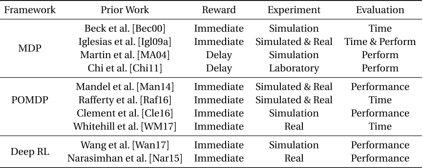
Table 2.1Reinforcement Learning Applications in Educational Domain
Framework Prior Work Reward Experiment Evaluation
MDP
Beck et al.[Bec00] Immediate Simulation Time Iglesias et al.[Igl09a] Immediate Simulated & Real Time & Perform
Martin et al.[MA04] Delay Simulation Perform
Chi et al.[Chi11] Delay Laboratory Perform
POMDP
Mandel et al.[Man14] Immediate Simulated & Real Performance Rafferty et al.[Raf16] Immediate Simulated & Real Time Clement et al.[Cle16] Immediate Simulation Performance
Whitehill et al.[WM17] Immediate Real Time
Deep RL Wang et al.[Wan17] Immediate Simulation Performance Narasimhan et al.[Nar15] Immediate Real Performance
2.2.4 Summarization of RL Applications in Educational Domain
Table 2.1 summarizes the related work about the RL applications in the educational domain. Al-though tabular MDP has the explainable state space and explicit rules which map a state into an action, it is challenging to construct an effective state space with the limited set of features, which di-rectly impact the effectiveness of MDP policies. While both POMDP and Deep RL have been shown to be highly effective in many real-world applications with high dimensional feature spaces, they generally require a great deal of training data, especially Deep RL. More importantly, it is often hard to interpret the induced POMDP and Deep RL policies.
Compared with previous research, we extensively explore both MDP and POMDP frameworks from three aspects including reward function, state representation, and policy execution. We also leverage the constraints into POMDP framework. Furthermore, we evaluate the effectiveness of in-duced RL policies using a series of the empirical experiments conducted in real classroom settings.
2.3
Constrained Reinforcement Learning
applied Bayesian RL algorithm to make the robot reach a target position as quickly as possible while avoiding dangerous places (say a crater) that might render them irretrievable. Garcia et al.[GF12] proposed the safe RL algorithm to explore the safe state space in dangerous and continuous control tasks.
The constrained RL problem can be transformed into the normal RL problem by assigning the negative or high cost for the particular actions that trigger constraints. Williams et al.[WY07] pro-posed the POMDP-based spoken dialogue system needs to successfully complete the task while minimizing the length of a dialogue by assigning the negative reward to the action which extended the length of the dialogue. Similarly, Hanheide et al.[Han17]assigned a unique cost to each action and applied the POMDP framework to induce the policy in a robot planning task, and tried to min-imize the cost of a policy, which is the linear combination of the cumulative cost for the executed actions and the cumulative reward for the goal state. Sanner et al.[San10]introduced the Relational Dynamic Influence Diagram Language to present the factored MDP or POMDP frameworks, and directly hard-coded constraints for each pair of states and actions to maintain the situation that the agent reached a legal state and executed a legal action at each step.
Some of prior work specified acost function, which is similar to the reward function and directly solves the constrained RL problem. For example, both Dolgov et al.[DD05]and Altman et al.[Alt99] applied the constrained MDP framework to induce the policy subject to the upper bound of the cumulative cost generated from the cost function. Furthermore, Kim et al.[Kim11]proposed the point-based value iteration approach to induce the policy based upon the constrained POMDP framework. Poupart et al.[Pou15]applied the linear programming approach to approximate the value functions of the state for both reward and cost. So far as we know, no prior work has directly sought to address the action-based constraints in the context of ITS.
2.4
Aptitude Treatment Interaction Effect
Previous work shows that the aptitude treatment interaction (ATI) effect commonly exists in many real-world studies. More formally, the ATI effect states that instructional treatments are more or less effective to individual learners depending on their abilities[CS77b]. For example, Kalyuga et al.[Kal03]empirically evaluated the effectiveness of worked examples (WE) vs. problem solving (PS) on student learning in programmable logic. Their results show that WE is more effective for inex-perienced students while PS is more effective for exinex-perienced learners.
with low prior knowledge: those who trained on the affect-sensitive tutor had significantly higher learning gain than their peers using the original tutor.
Chi et al.[CV10]investigated the ATI effect in the domain of probability and physics, and their results showed that the high incoming competence students can learn regardless of instructional interventions, while for students with low incoming competence, those who follow more effective instructional interventions learned significantly more than those following less effective interven-tions. In our prior work, it is consistently shown that for pedagogical decisions on WE vs. PS, certain learners are always less sensitive in that their learning is not affected, while others are more sensi-tive to variations in different policies. For example, Shen et al.[SC16b]trained students in an ITS for logic proofs, then divided students into the Fast and Slow groups based on time, and found that the Slow groups are more sensitive to the pedagogical strategies while the Fast groups are less sensitive.
CHAPTER
3
MARKOV DECISION PROCESS
3.1
Introduction
We explore the tabular MDP framework from three aspects includingreward function, state repre-sentation, and policy execution. This chapter is modified from papers published in[SC16a; She18b]. Reward Function. In general, real-world RL applications often contain two types of rewards: immediate reward, which is the immediate feedback after taking an action, and delayed reward, which is the reward received later after taking more than one action. The longer rewards are de-layed, the harder it becomes to assign credit or blame to particular actions or decisions. On the other hand, learning short-term performance boosts may not result in long-term learning gains. Thus, in this work we explore both immediate and delayed rewards in our policy induction, and empirically evaluate the impact of the induced policies on student learning. Our results show that using immediate rewards can be more effective than using delayed rewards.
selected feature set and then the option of selecting theleast correlated (Low option). The corre-lation in our case is calculated between features. Additionally, the high correcorre-lation-based option is commonly used for supervised learning where the features that are most highly correlated with the output labels, are often selected[YP97; LL06; CS14; Kop15]. Section 3.4.6 shows that indeed the high-correlation option outperformed two baseline methods: the random baseline and also the best feature selection explored in our previous work[Chi11]. However, for our dataset, the high option-selected features tend to be homogeneous. Different from the supervised learning tasks, we hypothesize that it is more important to have heterogeneous features in RL that can grasp different aspects of learning environments. Therefore, we also explore the low correlation-based option for feature selection with a goal to increase the diversity of the selected feature set. To do so, we select the next feature that is the least correlated with the current selected features to add to the the state representation. Our results show that the low correlation-based option significantly outperformed not only the high option but also the other two baselines.
Policy Execution.In most of the prior work with RL in ITSs, deterministic policy execution is used. That is, when evaluating the effectiveness of RL-induced policies, the system would strictly carry out the actions determined by the policies. In this work, we explorestochastic policy execu-tion. We argue that stochastic execution can be more effective than deterministic execution be-cause if the RL induced policy is sub-optimal, under the stochastic policy execution, it would still be possible for the system to carry out the optimal action; whereas if the induced policy is indeed optimal, our approach will make sure that when the decisions are crucial, the stochastic policy ex-ecution would behave like deterministic policy exex-ecution in that the optimal action will be carried out (see section 3.2.3 for details). We empirically evaluate the effectiveness of the stochastic policy execution but our results show that there is a ceiling effect.
The rest of this chapter is arranged as follows: Section 3.2 describes the reinforcement learn-ing framework and Markov Decision Process. Section 3.3 describes the tutorial decisions, Deep Thought tutor, our training data and state representation. Section 3.4 describes five correlation met-rics and then introduces our proposed feature selection methods. Section 3.5 presents the overview of our four empirical studies and research questions. Section 3.6 reports experimental results for each of the four experiments. Section 3.7 presents our post-hoc comparison results. Finally, we summarize our conclusions, limitations in Section 3.8.
3.2
MDP Framework
probability of transitioning from statesto states′by taking actiona. Finally, the reward functionR represents the immediate or delayed feedback:r(s,a,s′)denotes the expected reward of transition-ing from statesto states′by taking actiona. Since we apply the tabular MDP framework, reward functionR and transition probability table T can be easily estimated from the training corpus. The goal of an MDP is to generate the deterministic policyπ:s→athat maps each state onto an action.
3.2.1 Policy Induction
Once the tuple〈S,A,T,R〉is set, the optimal policyπ∗for an MDP can be generated via dynamic programming approaches, such as Value Iteration. This algorithm operates by finding the optimal value for each stateV∗(s), which is the expected discounted reward that the agent will gain if it starts ins and follows the optimal policy to the goal. Generally speaking,V∗(s)can be obtained by the optimal value function for each state-action pairQ∗(s,a)which is defined as the expected discounted reward the agent will gain if it takes an actiona in a states and follows the optimal policy to the end. The optimal state valueV∗(s)and value functionQ∗(s,a)can be obtained by iteratively updatingV(s)andQ(s,a)via equations 3.1 and 3.2 until they converge:
Q(s,a) := X s′
p(s,a,s′)r(s,a,s′) +γVt−1(s′)
(3.1)
V(s) := max
a Q(s,a) (3.2)
where 0≤γ <1 is a discount factor. When the process converges, the optimal policyπ∗can be induced corresponding to the optimal Q-value functionQ∗(s,a), represented as:
π∗(s) =a r g m a xaQ∗(s,a) (3.3)
whereπ∗is the deterministic policy that maps a given state into an action. In the context of an ITS, this induced policy represents the pedagogical strategy by specifying tutorial actions using the current state.
3.2.2 Policy Evaluation
The effectiveness of the MDP policy is estimated by Expected Cumulative Reward (ECR)[TL08; Chi11]. The ECR of a policyπis calculated by the average over the value function of initial states. It’s defined as:
E C R(π) =X i
Ni N ×V
π(S
i) (3.4)
initial states; andNi denotes the number of statesSias the initial states in the training corpus. In our case, the trajectories have a finite time horizon. Thus, ECR evaluates the expected reward of the initial states. The higher the ECR value of a policy, the better the policy is expected to perform.
3.2.3 Stochastic Policy Execution
The crucial part of stochastic policy execution is to assign a probability to each action. Note that in a policyπ, each actionafor a particular statesis associated with a Q-value, calledQπ(s,a)calculated by using equation 3.1 in Section 3.2. Thus, we transformQπ(s,a)into probabilitypπ(s,a)by the softmax function[SB98b], shown as follows:
pπ(s,a) = e
τ·Qπ(s,a)
P
a′eτ·Qπ(s,a′)
(3.5)
Hereτis a positive parameter, which controls the variance of probabilities for the state and action pair. Generally speaking, whenτ→0, the stochastic policy execution is close to random decision-making. Whenτ→+∞, the stochastic policy execution becomes deterministic. In order to determine the optimalτ, we use Importance Sampling[PS02]which can mathematically evalu-ate the effectiveness of policies with differentτvalues. Specifically, Importance Sampling (I S) of a policyπis formulated as follows:
I S(π|D) = 1 ND
ND
X
i=1
Li
Y
t=1
pπ(sti,ati) pd(si
t,ati)
·( Li
X
t=1
γt−1rti)
(3.6)
WhereNDdenotes the number of trajectories in the training corpusD;Li is the length of the ith trajectory;si
t,atiandrtiare the state, action and reward at thetth time step of theith trajectory respectively;pd(sti,ati)is the probability of taking the actionati for the statesti, calculated based on the other policyd, which generates the training corpusD. In our case, the decision in the train-ing corpus is randomly decided, thuspd(si
t,ati)always equal to 0.5. In general, the higher value of I S(π|D), the better policyπis supposed to be.
3.3
Pedagogical Decisions in a Logic Tutor: Deep Thought
3.3.1 Overview of Deep Thought
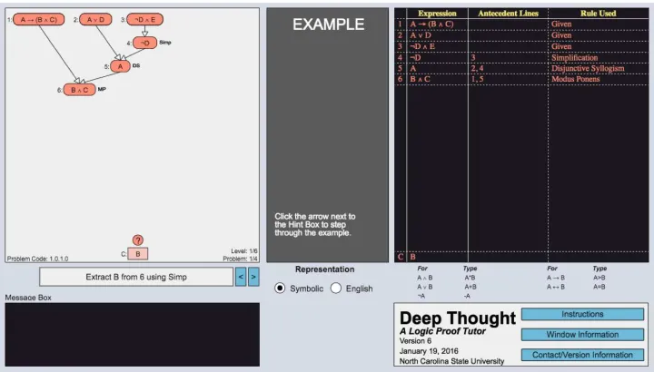
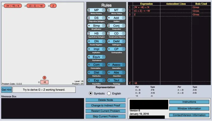
Deep Thought(DT) is a data-driven ITS used in the undergraduate-level Discrete Mathematics (DM) course at North Carolina State University (NCSU)[MB17]. DT provides students with a graph-based representation of logic proofs which allows students to solve problems by applying logic rules to derive new logical statements, represented as nodes. The system automatically verifies proofs and provides immediate feedback on rule application (but not strategy) errors. Every problem in DT can be presented in the form of either Worked Example (WE) or Problem Solving (PS). In WE (shown in Figure 3.1), students are given a detailed example showing the expert solution for the problem or were shown the best next step to take given their current solution state. In PS (shown in Figure 3.2), by contrast, students are tasked with solving the same problem using the ITS or completing an individual problem-solving step. Focusing on the pedagogical decisions of choosing WE vs. PS allows us to strictly control the content to beequivalent for all students.
Figure 3.1Interface for Worked Example
con-Figure 3.2Interface for Problem Solving
struction window on the left hand side of the tutor (shown in Figure 3.2). The hints are in the format of “Use expression X and expression Y to derive expression Z using rule”. Students are given the op-portunity to request hints on-demand by clicking the â ˘AIJGet Hintâ ˘A˙I button next to the dialogue box; however, if students stay in the current proof state for longer than the median step time of that problem or a maximum of 30 seconds, DT automatically presents the available hint. The WEs were constructed in a similar manner, where the most efficient (shortest-path) solution of the current proof from previous student solutions was used for a step-by-step presentation of the proof with procedurally constructed instructions given to the student below the proof window (Figure 3.2). At each step, the instructions for constructing the next step are presented in the same format as the next-step hints until the conclusion is reached.
The problems in DT are organized into six strictly ordered levels with 3–4 problems per level. Level 1 functions as apre-testin that all participants receive the same set of PS problems. In the five training levels 2–6, before the students proceed to a new problem, the system follows the cor-responding RL-induced or random policies to decide whether to present the problem as PS or WE. The last question on each level is a PS without DT’s help and thus functions as a quiz for evaluat-ing students’ knowledge of the concepts of that level. After completevaluat-ing the entire trainevaluat-ing in DT, students take a in-class exam, referred as thetransfer post-test.
241,p=.005. Therefore, when comparing the transfer post-test scores in the following, we used ANCOVA tests with pre-test scores as the covariate.
Finally, note that when inducing RL policies using training data set, reward functions are gen-erated based on level scores because there was a significant positive correlation between students’ level scores and transfer post-test scores. Given that the ultimate goal of the DT tutor is to improve students’ performance in the real classroom exam, the transfer post-test score, in the following we used the transfer post-test score to evaluate students’ learning performance and to investigate the effectiveness of pedagogical policies.
3.3.2 Two Training Datasets:
DT-Imme
andDT-Delay
Our training dataset was collected in the Fall 2014 and Spring 2015 semesters, with a total of 306 students involved. All students were trained on DT where whether to present the next problem as a WE or a PS wasrandomly decided. The average number of problems solved by students was 23.7 and the average time that each student spent in the tutor was 5.29 hours. In addition, we calculated students’ level scores based on their performance on the last problem in each of levels 1–6. For the sake of simplicity, level scores were normalized to[0, 100]. If the students quit the tutor during the training, we assigned a strong negative reward, -300 in this case, on the last problem they attempted. Furthermore, theimmediate rewardwas defined as the difference between the current and previ-ous level scores, and thedelayed rewardwas defined as the difference of the level scores between level 1 and 6. From the interaction logs, we represent each observation using a high-dimensional feature space introduced in the following section. Combing observation with two types of rewards, we construct two different types of training datasets namedDT-ImmeandDT-Delayrespectively.
3.3.3 Feature Set
A total of 133 state features were extracted from the DT log files. They include 45 categorical features and 78 continuous features that can be grouped into five categories listed as follows:
1. Autonomy (AM).This category relates to the amount of student work done. For example, in-teractiondenotes the cumulative number of student clickstream interactions andhintCount denotes the number of times a student clicked the hint button during problem solving. There are a total of 12 features in the AM category, including 8 categorical and 4 continuous features.
3. Problem Solving (PS).This category encodes information about the current problem solv-ing context. For example,probDiff is the difficulty of the current solved problem;NewLevel indicates whether the current solved problem is in a new level in the tutor. There are a total of 30 features in the PS category, including 13 categorical and 17 continuous features.
4. Performance (PM).This category describes information about the student’s performance during problem solving. For example,RightAppdenotes the number of correct rule appli-cations. There are a total of 36 features in the PM category, including 24 categorical and 12 continuous features.
5. Student Action (SA).This category is a tutor-specific category for DT. It evaluates the sta-tistical measurement of students’ behavior. For instance,actionCountdenotes the number of non-empty-click actions that students take;AppCount denotes the number of clicks for derivation of a logical expression. There are a total of 32 continuous features in the SA cate-gory.
Before feature selection and policy induction, we discretized the continuous features by explor-ing k-means clusterexplor-ing first and then a simple median split. The latter is conducted only if we failed to get balanced clusters from the former. More specifically, the general discretization process is 1) Given a continuous feature, we start by using k-means with k equal to 5 and generate the clusters; 2) if the size of the clusters are not balanced, we reduce the value of K, until balanced clusters are constructed; 3) Finally, if k equals 1, we use median split to discretize the feature.
In this work, we focus on applying different feature selection approaches to generate a small set of features to construct the state space in a tabular MDP framework. By doing so, we can shed some light on what the most important features are for decision-making on PS vs. WE. Moreover, when applying RL in real-world scenarios, we may not always have the full computation power to track all of the features at once. Next, we describe the feature selection approaches in Section 3.4.
3.4
Feature Selection on the MDP Framework
divided by the total number of the student entries, or "Number of Correct" defined as the num-ber of the correct student entries, or "Numnum-ber of Incorrect" defined as the numnum-ber of the incorrect student entries and so on. When making specific decisions about including a feature on student knowledge level in the state, for example, it is often not clear which of these features should be in-cluded. Therefore a more general state representation approach is needed. To this end, this project began with a large set of features to which a series of feature-selection methods were applied to reduce them to a tractable subset.
3.4.1 Related Work For Feature Selection in RL
Much previous work on feature selection for RL mainly focused on model-free RL. Model-free al-gorithms learn a value function or policy directly from the experience while interacting with the agent.[KN09]applied Least-Squares Temporal Difference (LSTD) withLassoregularized items to approximate the value function as well as to select an effective feature subset. Similarly,[Kel06] applied LSTD to approximate a value function and select a feature subset by implementing Neigh-borhood Component Analysisto decompose approximation error, which can be used to evaluate the efficacy of the feature subset.[Bac09]explored the penalization of an approximation function by usingMultiple Kernel learning. Additionally,[Wri12]proposed the feature selection embedded in a neuro-evolutionary function which approximates the value function, and they selected each feature based on its contribution to the evolution of network topology.
[Chi11]previously investigated 10 feature selection methods, calledRLpre-FS(Sec. 3.4.4). These methods were implemented to derive a set of various policies, where features are mostly selected based on the single feature’s performance or covariance in training data. The results showed there was no consistent winner and in some particular cases these methods perform no better than the random baseline method.
Different from prior work, our features are selected based on the correlations through two steps: 1) a new feature is selected based on its correlation with the current “optimal" subset of features; 2) for different sets of state features, the sameA,R and training data are used for estimatingT when applying MDP to induce policies and ECR is used to evaluate the induced policies.
3.4.2 Five Correlation Metrics
Our feature selection methods involve five correlation metrics. The first four are commonly used in supervised learning and here we will investigate whether they can be effectively applied for feature selection in RL. We propose the fifth metric, called Weighted Information Gain (WIG), by combin-ing the first four metrics and adaptcombin-ing them based on the characteristics of our data sets. More specifically, we have:
two variables: whether the distribution of a categorical variable differs significantly from an-other categorical variable.
2. Information gain (IG)[LL06]: measures how much information we would gain about a vari-ableY if knowing another variableX. It is calculated as:
I G(Y,X) =H(Y)−H(Y|X) (3.7)
whereH(·)is the entropy function – measuring the uncertainty of a variable. IG(Y, X) evaluates how the uncertainty of a variableY would change from knowing the variableX. To some extent, it can also be treated as a type of correlation betweenX andY. Note that IG has the bias towards the variable with a large number of distinct values.
3. Symmetrical uncertainty (SU)[YL03]: it is defined as:
SU(Y,X) =H(Y)−H(Y|X)
H(X) +H(Y) (3.8)
SU evaluates the correlation between two variablesY andX by normalizingI G(Y,X). SU compensates for the weakness of IG by considering the uncertainty of both variablesX and Y in the denominator.
4. Information gain ratio (IGR)[Ken83]: is the ratio of information gain to the intrinsic informa-tion, which is the entropy of conditional information. IGR can be represented as:
I G R(Y,X) =H(Y)−H(Y|X)
H(X) (3.9)
Compared with SU, IGR only considers the uncertainty of variableX in the denominator.
5. Weighted Information gain (WIG) is proposed as:
W I G(Y,X) = H(Y)−H(Y|X)
(H(Y) +H(X))·H(X) (3.10)
WIG can be seens as a combination of IG, SU and IGR. Compared to SU, WIG sets more weight onXby multiplyingH(X)in the denominator while compared to IGR, WIG normalizes IG by considering the uncertainty of both variablesX andY.
the high correlation-based option is commonly used for supervised learning where the features that are most highly correlated with the output labels are often selected[YP97; LL06; CS14; Kop15]. However, for RL, the high option-selected features tend to be homogeneous. Different from the su-pervised learning tasks, we hypothesize that it is more important to have heterogeneous features in RL that can grasp different aspects of learning environments. Therefore, we also explore the low correlation-based option for feature selection with a goal to increase the diversity of the selected feature set. As a result, we have 10 correlation-based methods named: CHI-high, IG-high, SU-high, IGR-high, WIG-high, CHI-low, IG-low, SU-low, IGR-low, and WIG-low. Our goal is to investigate which option is better: high vs. low, and which of the five correlation metric performs the best.
3.4.3 Correlation-based Feature Selection Approaches
Algorithm 1Correlation-based Feature Selection Algorithm
Require: Ω: Feature space;D: Training data;N: Maximum number of selected features Ensure: S∗: Optimal feature set
1: for fiinΩ do
2: ECRi←CALCULATE-ECR(D, fi)
3: end for
4: Addf∗with highestECRtoS∗
5: whileSIZE(S∗)<N do
6: for fiinΩ− S∗ do
7: Ci←CALCULATE-CORRELATION(S∗,fi,m) 8: end for
9: F ←SELECTTOP(C, 5, reverse) ⊲Select top 5 features based on correlation metrics
10: for fiinF do
11: ECRi←CALCULATE-ECR(D,S∗+fi)
12: end for
13: ReplaceS∗byS∗+fiwith higgestECR
14: end while
Algorithm 1 shows the process of our correlation-based feature selection method. It contains three major parts. In the first part (lines 1–4), the algorithm constructs MDPs for every single feature inΩ, induces a single-feature policy and calculates itsE C R(defined in Sect. 3.4). Then the feature with highestE C R is added to the current optimal feature setS∗. In the second part (lines 6–9), the algorithm follows a forward step-wise feature selection procedure in that, given the currently selected feature setS∗, it selects the next feature based on the five correlation metrics described above. More specifically, it first calculates the correlations betweenS∗with each featuref
highest correlations for high-option or the bottom 5 lowest features for low options, decided by the Boolean variablereversein line 9. These features are selected to form a feature poolF. In the third part (lines 10–13), the currentS∗is combined with each featurefi∈ Fto induce a policy and C a l c u l a t e-E C R function calculates theE C R of the induced policy. ThenS∗+f
k, the combi-nation that produces the policy with the highestE C R, will be the newS∗for the next round. The algorithm will terminate when the size of an optimal feature set reaches maximum numberN.
3.4.4 PreRL-FS Approach
Chi et al.[Chi11]developed a series of feature selection approaches, referred asPreRL-FSin the following. They can be grouped into three categories: 1) four ECR-based methods, which use ECR, Upper-Bound, Lower-Bound of ECR, or Hedge value of the single-feature policy as the feature selec-tion criteria. In particular, the Upper-Bound and Lower-Bound of ECR refer to the 95% confidence interval for ECR, and Hedge is defined asH e d g e =E C R/(U p p e r B o u n d−L o w e r B o u n d); 2) two PCA-based methods, which select features that are highly correlated with principal compo-nents; and 3) four ECR & PCA-based methods, the combination of the former two approaches. The results indicated that thefour ECR-based methods outperformed the other two types of ap-proaches in terms of ECR.
Algorithm 2Ensemble Feature Selection Algorithm Require:
Ω: Feature space;D: Training data;N: Maximum number of selected features; M: A set of feature selection approaches.
Ensure: S∗: Optimal feature set
1: for fiinΩ do
2: ECRi←CALCULATE-ECR(D, fi)
3: end for
4: Addf∗with highestECRtoS∗
5: whileSIZE(S∗)<N do
6: F ← ;
7: for Methodk inM do
8: Fk←SELECT-FEATURE(D,Ω− S∗,Methodk)
9: F ← F ∪ Fk
10: end for
11: for fiinF do
12: ECRi←CALCULATE-ECR(D,S∗+fi)
13: end for
14: ReplaceS∗byS∗+fiwith higgestECR
3.4.5 Ensemble Approach
Algorithm 2 shows the basic process of our ensemble feature selection procedure, which is simi-lar to that of correlation-based methods. The major difference is in the second part (lines 6–10). Our ensemble approach explored a total of 12 feature selection methods are referred to asM in Algorithm 2: the fourECR-basedmethods which are the better methods among thePreRL-FS ap-proaches and the eight out of the 10 proposed correlation-based methods (WIG-high and WIG-low were excluded here because they were not explored when we first explored the ensemble approach). More specifically, the ensemble approach integrates the featuresFkgenerated from each of feature selection methodMethodkinMand generates a relatively large feature poolF. The maximum size ofF can be up to 70, but often much smaller because of the overlapping of feature sets generated from different methods. Note that the feature pool is still much larger than any of our 10 correlation-based methods, which is 5. After generating the feature pool, the ensemble method carries out the same procedure, the third part (lines 11–13), as the correlation-based methods described above. Although the ensemble method has a relatively high computational complexity, it has a wider ex-ploration of the feature space by integrating different types of feature selection methods.
3.4.6 Comparison Results for Feature Selection Approaches
We explore three categories of feature selection approaches:PreRL-FS, ensemble, and high- and low- correlation-based approaches and compare them against a random feature selection baseline. We use ECR (Section 3.4) to theoretically evaluate the effectiveness of the MDP policies, which indi-rectly verify the effectiveness of feature selection approaches. Note that ECR is calculated based on the induced MDP policies and the two training datasets: DT-Immed and DT-Delay (Section 3.3.2).
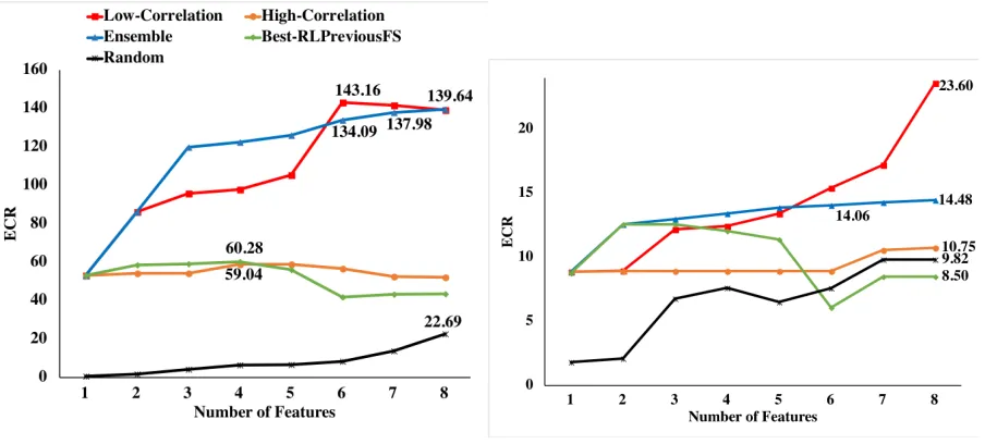
High VS Low Correlation-based Approaches.Figure 3.3 and Figure 3.4 show the ECR values of 10 correlation-based methods on DT-Immed and DT-Delay respectively, where the y-axis repre-sents the value of the ECR of the induced policy given the selected features, and the x-axis denotes the number of features (maximum is 8). Note that all feature selection methods start in the same place atx=1 except the random method. This is because all methods will initially select the feature with the best ECR of single-feature policy. However, ECR values vary dramatically as the number of selected features increases. The solid line indicates the performance of the low correlation-based approaches and the dotted line denotes the performance of the high correlation-based version. In addition, the ECR value of policies using immediate reward is much higher than that of policies using the delayed reward.
Figure 3.5DT-Immed Figure 3.6DT-Delay
Five Correlation Metrics.Figures 3.3 and 3.4 show that WIG is the consistently highest per-former in that it has the best ECR for both DT-Immed and DT-Delay datasets. CHI performed well in DT-Immed dataset while IGR performed well in DT-Delay dataset. In short, our proposed WIG performed best among all the five correlation metrics.
Overall Comparison.Figures 3.5 and 3.6 show the overall comparison among all methods on DT-Immed and DT-Delay data respectively. Particularly, with the purpose of simplicity, for both low and high correlation-based methods and the PreRL-FS methods, we selected the best method from each category. In other words, the figures present a comparison among the five methods in-cluding the best of five Low-correlations, the best of five High-correlations, ensemble, the best of PreRL-FS, and the random approach. Results show that, as expected, the random method performs worst across the two datasets. In addition, the best of the high correlation-based methods outper-forms random and Best-RLPreviousFS approaches when the number of features is above 5. The best of the low correlation-based methods outperforms other methods. In general, the best low correlation-based method outperforms the best ofPreRL-FSby an average of 43.87% and outper-forms the ensemble method by an average of 9.05%. In addition, the ensemble method improves over the best ofPreRL-FSby an average of 36.46%. The value of ECR does not always rise as the the number of features increases. The ECR of the low-correlation approach decreases a lot when increasing the number of features from 6 to 8. The ECR of the ensemble method seems to converge when the number of features is more than 6 for both two training datasets. The ECR of the best of PreRL-FSdecreases when the number of features is more than 4.
In summary, based on ECR results we can rank five categories of methods as Low correlation-based>Ensemble>High correlation-based≈PreRL-FS≫Random. In particular, the WIG-Low approach performs best among all implemented approaches.
3.5
Experiments Overview
3.5.1 Research Questions
In this work, we investigate the effectiveness of RL-induced policies using the MDP framework from three aspects: state representation using different feature selections, reward function, and policy execution options. For each aspect, we have a corresponding research question and thus our three research questions are listed as follows:
• Q1 (State):Can effective feature selection methods empirically improve the effectiveness of the induced policy?
• Q3 (Execution):Can stochastic policy execution be more effective than deterministic policy execution?
3.5.2 Reinforcement Learning Policies
Table 3.1 lists the five RL policies induced for investigating the three research questions above. All five policies were induced using the MDP framework but involved different types of feature se-lection methods (the second column), reward function (the third column), and/or policy execu-tion (the fourth column). The last column shows that the ECR of the RL-induced policies. More specifically,MDP-ECRis induced by using MDP with the best PreRL-FS feature selection approach; Ensemble-ImmeandEnsemble-Delayare two policies induced with the ensemble feature selection approach using immediate and delayed reward respectively; andWIG-detandWIG-stowere both induced using WIG with the low-correlation option for feature selection, and the main difference is that the former is executed deterministically while the latter is executed stochastic. Note that becauseWIG-stois a stochastic policy and because ECR can only be calculated for a deterministic policy, the ECR ofWIG-stois listed as “NA".
Table 3.1Reinforcement Learning Policies in Four Experiments
Policy Feature Selection Reward Execution ECR
MDP-ECR ECR-based Immediate Deterministic 60.28
Ensemble-Imme Ensemble Immediate Deterministic 137.98
Ensemble-Delay Ensemble Delay Deterministic 14.06
WIG-det Low Corre-based Immediate Deterministic 143.16
WIG-sto Low Corre-based Immediate Stochastic NA
Note: ECR is only used for evaluating the deterministic policies
3.5.3 Experiments Overview