Search | Preprints

(1)

Article

1 An Approximation Method of Fuzzy Numbers Based on Extended Fuzzy Transforms

2

Ferdinando Di Martino 1,2*_{, Salvatore, Sessa}1,2

3

1 _{Università degli Studi di Napoli Federico II, Dipartimento di Architettura, Via Toledo 402,}

4

80134 Napoli, Italy

5

2 _{Università degli Studi di Napoli Federico II, Centro Interdipartimentale di ricerca A. Calza Bini,}

6

Via Toledo 402, 80134 Napoli, Italy

7

8 *

Correspondence: [email protected]; Tel.: +39-081-253-8904

9

10

11

12

Abstract: We propose a new Mamdani fuzzy rule-based system in which the fuzzy sets in the

13

antecedents and consequents are assigned in a discrete set of points and approximated by using the extended

14

inverse fuzzy transforms, whose components are calculated by verifying that the dataset is sufficiently dense

15

with respect to the uniform fuzzy partition. We test our system in the problem of spatial analysis consisting in

16

the evaluation of the liveability of residential housings in all the municipalities of the district of Naples (Italy).

17

Comparisons are done with the results obtained by using trapezoidal fuzzy numbers in the fuzzy rules.

18

Keywords: Extended fuzzy transform, fuzzy number, rule management system, spatial

19

analysis

20

21

1. Introduction

22

The A fuzzy number (FN) is a fuzzy set with membership function A: Reals →[0,1] defined as

23

0 IF x a

A (x) IF a

A( ) 1 IF

A (x) IF d

0 IF x b x c

x c x d

x b          _    _ _     (1)

where a ≤ c ≤ d ≤ b, A- _{: [a,c]}_→_{[0,1] is a not decreasing continuous function with}

24

A-_{(a) = 0, A}-_{c) = 1 and A}+ _{: [b,d]}_→_{[0,1] is a not increasing continuous function with A}+_{(d) = 1,}

25

A+_{(b) = 0. A}-_{and A+ are called left-side and right side of A, respectively.}

26

Complicated left-side and right-side functions can generate serious computational difficulties

27

when imprecise information is modeled by FNs. In order to overcome this problem, the original FN

28

can be approximated with other easier functions. The simplest FNs used in fuzzy modeling,

29

fuzzy control and fuzzy decision making are the trapezoidal and triangular FNs. In a trapezoidal FN

30

the functions A-_{and A}+_{are linear: for instance,}

31

A-_{(x) = (x-a)/(c-a) and A}+_{(x) = (b-x)/(b-d) with a≤b≤c≤d, a≠c, b≠d. In a triangular FN it is assumed}

32

d=c. Other simple FNs widely used is the degenerated left (resp., right) size semi-trapezoidal FNs

33

with a = c < d < b (resp., a < c < d = b). In many problems trapezoidal, triangular or semi-trapezoidal

34

approximations of FNs could give a loss of information not negligible and this can significantly

35

affect the reliability of the results.

36

Furthermore, the membership functions of FNs used in applications are not generally known:

37

for example, when they are obtained as relative frequencies of measured occurrences in in a discrete

38

set of points, or in collaborative applications in which a set of stakeholders evaluate separately the

39

membership degrees of a FN and the function is assigned as an average of these membership

40

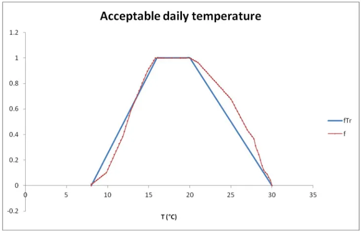
degrees. For making understandable this idea, in the example of Fig 1 the membership degree f(T) of

41

(2)

the fuzzy set “daily temperature T” (measured in °C) for a discrete set of 100 points is the average of

42

the membership degrees evaluated separately by many stakeholders.

43

44

45

Fig. 1. Example of FN constructed for a discrete set of points and approximated with a trapezoidal

46

membership function

47

Recently many methods are proposed in order to approximate FNs with easier FNs using a

48

suitable metric (see, e.g. [1, 6, 23, 29, 30, 31]). Some authors investigate approximations by adding

49

some restrictions to preserve properties of a FN as core [2], ambiguity [3, 4, 5], expected interval,

50

translation invariance and scale invariance [19, 20]. As pointed out in [8], by using a trapezoidal

51

FN as approximation function by, only a limited number of characteristics can be preserved since a

52

trapezoidal FN depends only by four parameters, and the best approach to preserve multiple

53

characteristics is to use sequences of FNs. In [7] a new method is proposed based on the inverse

54

fuzzy transform (iF-transform) [24] in order to construct sequence of FNs which converge uniformly

55

to a FN, preserving properties as its support, core, ambiguity, quasi-concavity and expected interval.

56

The F-transform method was already used image analysis (see, e.g. [10, 13, 14, 26, 27]), data

57

analysis applications (see, e.g. [11, 12, 15, 25]). In [28] the bi-dimensional F-transform is used to

58

approximate type-2 FNs. In [7] the extended iF-transform method, proposed in [27], is applied to

59

approximate FNs preserving the support and the quasi-concavity property. The main advantage of

60

this method is to reach the desired approximation with a linear rate of uniform convergence.

61

However, when the membership function is given in a discrete set of point, it is necessary to verify

62

that this dataset is sufficiently dense with respect to the uniform fuzzy partition of the support of the

63

FN. More specifically, the F-transform method divides the interval [a,b] in n sub-intervals of width

64

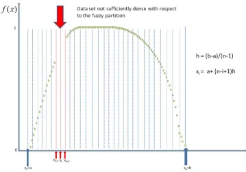
h = (n-1)/(b-a). The points x1= a, x2= a+h,..., xi= a+(i-1)h,..., xn= b are called nodes: an uniform fuzzy

65

partition of [a,b] is created by assigning n fuzzy sets with continuous membership functions A1,…,An

66

: [a,b] → [0,1], called basic functions, where Ai(x) = 0 if x(xi-1,xi+1), i = 1,....,n. When the input

67

data form a dataset of points in [a,b], it is necessary to control that this set is dense with respect to

68

the uniform fuzzy partition, namely we must verify that at least one data point with non-zero

69

membership degree falls within a sub-interval (xi-1,xi+1) for i=1,...,n. In Fig. 2 we show an example

70

of dataset not sufficiently dense with respect to the fuzzy partition: no data is included in (xi-1,xi+1).

71

(3)

74

Fig. 2. Example of input dataset non sufficiently dense with respect to the fuzzy partition.

75

The paper is organized as follows: Section 2 contains the basic notions of fuzzy number and

76

F-transform, in Section 3 we introduce the extended iF-transform method which in Section 4 is

77

applied to a Fuzzy Rule Based Systems (FRBS). In Section 5 we give the results of our tests and final

78

considerations are reported in Section 6.

79

80

1.1 Preliminaries

81

As already shown in [11, 12], the extended iF-transform method, proposed in [7], approximates

82

a function assigned on a discrete set of points by means of an iterative process. Strictly speaking,

83

we set initially the dimension n of the fuzzy partition to a value n0, afterwards it is necessary to

84

verify at any step that the dataset is sufficiently dense with respect to the fuzzy partition and that the

85

approximation error is less or equal to a prefixed threshold: in this case the process stops and the

86

direct F-transform components are stored, otherwise n is set to n + 1 and the process is iterated by

87

considering a finer fuzzy partition. Below we schematize the pseudocode of this process.

88

We propose a new Mamdani FRBS in which we use the extended iF-transform to approximate

89

FNs and we apply the above process for constructing the input fuzzy sets in the antecedent and the

90

output fuzzy sets.

91

92

Approximation of a set of data by using the extended inverse F-transform 1 n:=n0

2 Create the fuzzy partition

3 Calculate the direct F-transform components

4 WHILE the dataset is sufficiently dense with respect to the fuzzy partition 5 Calculate the approximation error

(4)

9 END IF

10 n:=n+1

11 Calculate the extended direct F-transform components

12 END WHILE

13 RETURN “ERROR: Dataset not sufficiently dense”

14 END

93

The extended iF-transform method for approximation of the FNs is used to fuzzify the crisp

94

input data. The min and max operators are applied as AND and OR connectives in the

95

antecedent of the fuzzy rules to calculate the strength of any rule. The defuzzification process of the

96

output fuzzy set is carried out via the discrete Center of Gravity (CoG) method. For example, we

97

consider a system formed by two rules in the form:

98 















1 1 1 1

2 2 2 2

: is A OR is B is C

: is A AND is B is C

r x y z

 

 

 



(2)

where A1 and A2 are two FNs for the linguistic input variable x, B1 and B2 are two FNs for the

99

input linguistic variable y, C1 and C2 are two FNs for the output variable z. Applying the extended

100

iF-transforms to evaluate each fuzzy set, we suppose thatA1

 

x 0.4,A1

 

x 0.7,B1

 

x 0.7,

101  

2 0.3.

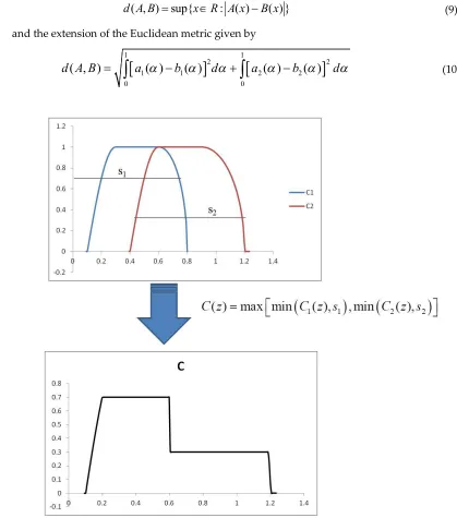
B x  With max (resp., min) operator as connective OR (resp., AND), we obtain the value of

102

the two rules: r1 = max(0.4, 0.7) = 0.7 and r2 = min(0.7, 0,3) = 0.3. In the defuzzification process we

103

reconstruct the output fuzzy set as

104 

1 1





2 2



( ) max min ( ), , min ( ),

C

f z  _ C z s C z s _ ₍₃₎

The CoG method is useful for obtaining the final crisp value

z

ˆ

of the output variable as

105

1 1

ˆ ( ) ( )

Nc Nc

i i i

i i

z C z z C z

 



_



_

(4)

where Nc is the number of rules and z1< z2 <…< zNc are points of the support of C. In Fig. 3 we

106

give an example.

107

108

2. Fuzzy Numbers and F-transforms

109

2. 1 Fuzzy Numbers and F-transforms

110

Given a value α ∈ [0,1], we denote with A, called α-cut of a FN A, the crisp set containing the

111

elements x_{R with a membership degree greater or equal to α. We also use the interval}

112

1 2

[ ]A_ [a ( ), a ( )]



(5)

Where

113 



1( ) inf : ( )

a   xR A x  ₍₆₎





2( ) sup : ( )

a   xR A x  ₍₇₎

For α = 1, [A] =[a (1),a (1)]₁ ₁ ₂ is called the core of the FN and denoted by core(A).

114

(5)





supp( )

A



x



R A x

| ( )



0

(8)

Given two arbitrary FNs A and B, two metrics are considered in [17, 18]:

116

the Chebyshev distance

117

( , ) sup{ : ( ) ( ) }

d A B  xR A x B x (9)

and the extension of the Euclidean metric given by

118 







1 1

2 2

1 1 2 2

0 0

( , )

( )

d A B



_

a





b



d





_

a





b



d



(10)

119

120

Fig. 3. Defuzzification of the output fuzzy set

121

122

Two properties of A are given in [9] called Ambiguity and Value defined as

123 



1

2 1

0

( ) ( ) ( ) ( )

r

Amb A 

_

r



 a



a



d



(11)

(6)





1

2 1

0

( ) ( ) ( ) ( )

r

Val A 

_

r



 a



a



d



(12)

respectively, where r: [0,1]→[0,1] is a not decreasing function called reducing function with

125

with r(0) = 0 and r(1) = 1. Another important propriety is the Expected Interval of A, introduced in

126

[16, 21], defined as follows

127

1 1

1 2

0 0

( ) ( ) , ( )

EI A   a

 

d a

 

d 

 







(13)

We have EI(A) = [(a+c)/2, (d+b)/2] for a trapezoidal FN A.

128

2. 2 Direct and Inverse F-transforms

129

Following the definitions and notations of [24], let n ≥ 2 and P = {x1, x2, …, xn} be a set of

130

points of [a,b], called nodes, such that x1 = a < x2 <…< xn = b. Let {A1,…,An} be an assigned family of

131

fuzzy sets with membership functions A1(x),…,An(x): [a,b] → [0,1], called basic functions. We say

132

that it constitutes a fuzzy partition of [a,b] if the following properties hold:

133

134

(1) Ai(xi) =1 for every i =1,2,…,n;

135

136

(2) Ai(x) = 0 if x (xi-1,xi+1) for i=2,…,n;

137

138

(3) Ai(x) is a continuous function on [a,b];

139

140

(4) Ai(x) strictly increases on [xi-1,xi] for i = 2, …, n and strictly decreases on [xi,xi+1]

141

for i = 1,…, n-1;

142

(5)

n

i i=1

A(x)=1

_

for every x[a,b].

143

144

Furthermore, we say that the fuzzy sets {A1,…,An} form an h-uniform fuzzy partition of [a,b] if

145

146

(6) n ≥ 3 and xi = a + h∙(i-1), where h = (b-a)/(n-1) and i = 1, 2, …, n (that is the nodes are

147

equidistant);

148

149

(7) Ai(xi – x) = Ai(xi + x) for every x[0,h] and i = 2,…, n-1;

150

151

(8) Ai+1(x) = Ai(x- h) for every x[xi,xi+1] and i = 1,2,…, n-1.

152

153

Let f(x) be a continuous function on [a,b]. The following quantity

154

( ) ( ) ( )

b b

i i i

a a

F  f x A x A x (14)

for i = 1, …, n, is the ith component of the direct F-transform [F1, F2, …, Fn] of f with respect

155

to the family of basic functions {A1, A2, …, An}. If this fuzzy partition is h-uniform, the

156

(7)

2 1 1 1 1 1 1 1

2 ( ) ( ) 1

( ) ( ) 2,..., 1

2 ( ) ( )

x x xi i i xi xn n xn

h f x A x dx if i

F h f x A x dx if i n

h f x A x dx if i n

            _ _      _    (15)

The following function

158

,

1

( ) ( )

n F n i i

i

f x F A x



  (16)

where x_{[a,b], is defined the iF-transform of f with respect to {A1, A2, …, An} and it}

159

approximates f in the sense of the following theorem [24]:

160

161

Theorem 1. Let f(x) be a continuous function on [a,b]. For every ε > 0, then there exist an

162

integer n(ε) and a fuzzy partition {A1, A2, …, An(ε)} of [a,b] such that |f(x) - fF,n(ε)| < ε with respect to

163

the existing fuzzy partition.

164

165

In the discrete case we know that the function f assumes assigned values in the points

166

p1,...,pm of [a,b],. If the set {p1,...,pm} is sufficiently dense with respect to the fixed partition {A1, A2,

167

…, An}, that is for each i = 1,…,n there exists an index j{1,…,m} such that Ai(pj) > 0, we can

168

define the n-tuple {F1, F2,…, Fn} as the discrete direct F-transform of f with respect to {A1, A2, …,

169

An }, where each Fi is given by

170

1 1

( ) ( ) ( )

m m

i j i j i j

j j

F f p A p A p

 

    ₍₁₇₎

for i=1,…,n. Similarly we define the discrete iF-transform of f with respect to the {A1, A2,

171

…, An} by setting

172

,

1

( ) n ( )

F n j i i j i

f p F A p



  (18)

for every j_{{1,…,m}. We have the following theorem [24]:}

173

174

Theorem 2. Let f(x) be a function assigned on a set of points {p1,..., pm}[a,b]. Then for every

175

ε > 0, there exist an integer n(ε) and a related fuzzy partition {A1, A2, …, An(ε)} of [a,b] such that

176

{p1,...,pm} is sufficiently dense with respect to the existing fuzzy partition and for every pj_{[a, b], j =}

177

1,…,m, the following inequality

178

|f(pj) - fF,n(ε) (pj) | < ε (19)

remains true.

179

3. The extended iF-transform and fuzzy numbers

180

In [27] the extended iF-transform of a continuous function f is introduced in order to preserve

181

the monotonicity as follows. For an h-uniform fuzzy partition {A1, A2, …, An}, the function f is

182

extended to [a-h,b+h] as follows:

183

2 ( ) (2 ) if x [a-h,a] ( ) ( ) if x [a,b]

2 ( ) (2 ) if x [b,b h]

f a f a x

f x f x

f b f b x

     _   _ _ _ _  (20)

(8)

1 1

1

(2 ) if x [a-h,a]

( )

( ) if x [a,a h]

( ) ( ) for i = 2,...,n-1

( ) if x [b-h,b] ( ) (2 ) i _i n n n

A a x

A x

A x A x

A b x

          

 if x [b,b h] 



 



(21)

Then the ith component Fi of the extended direct F-transform of f with respect to the family of

185

basic functions {A1, A2, …, An} is given by

186

1 ₁

1

f ( ) ( ) , h

( ) ( ) 2,.., 1

1 ( ) ( ) h a h a h i _i b h n _n b h

F x A x dx

F x F x i n

F f x A x dx

        



(22)

Hence the extended iF-transform of f is given by

187 



1 , 1 1

2

fF n( ) ( ) n i i( ) nA ( ) xn a-h, b

i

x F A x  F A x F x h



     (23)

By [8, Lemma 9], we obtain that

188

1 , , ( ) ( ) ( ) ( ) F n n F n

f a F f a

f b F f b

 

  (24)

Let S be a fuzzy number with a continuous membership function and supp(S) = [a,b]. We

189

consider an h-uniform fuzzy partition {A1, A2, …, An} of [a,b] with n ≥ 3 and let SF n, ( )x be the

190

extended iF-transform of S. We obtain that [8, Prop. 11]:

191

, ,

SF n(a)SF n( )b 0

,

SF n( )x 0  x ( , )a b 1

,

2 SF n( ) n i i( )

i

x  S A x

  

(25)

where Si is the ith component of the direct F-transform of S (cfr., formulae (15)). Theorem 13 of

192

[8] provides the approximation property of the extended iF-transform as follows.

193

194

Theorem 3. Let S be a FN having a continuous membership function and supp(S) = [a,b]. Let a

195

fuzzy partition {A1, A2, …, An} of [a,b] be h-uniform with n ≥ 3 and SF n, ( )x be the extended

196

iF-transform of S calculated by (23). Then the following inequality holds:

197

, [ , ]

sup SF n( ) ( ) 2 ( , )

x a b

x S x



S h



  ₍₂₆₎

where ω(S,h) is the modulus of continuity of S given by

198

, [ , ]:

2 ( , )



S h



sup

_{x y}__{a b a b h}_{ }

S x

( )



S y

( )

₍₂₇₎

Another important theorem [8, Th. 14] proves that the extended iF-transform preserves the

199

shape and the approximation properties of a FN as follows.

200

(9)

Theorem 4. Let S be a FN having a continuous membership function, supp(S) = [a,b] and

202

core(S) = [c,d], a < c < d < b. Let a fuzzy partition {A1, A2, …, An} of [a,b] be h-uniform with n ≥ 3 and

203

a fuzzy set T such that T(x) = SF n, ( )x calculated by (23) in [a,b] and T(x)=0 if x[a,b]. If h =

204

(b-a)/(n-1) is such that h ≤ min{(d-c)/4, c-a, b-d}, then T is a FN for which the following hold:

205

206

supp(T) = supp(S);

207

If core(T) = [c’,d’], then c ≤ c’ ≤ d’ ≤ d, |c-c’| ≤ 2h, |d-d’| ≤ 2h;

208

[ , ]

sup ( ) ( ) 4 ( , )

x a b

T x S x  S h



 

;

209

If S-_{strictly increases on [a,c], then T strictly increases on [a,c’];}

210

If S+_{strictly decreases on [d,b], then T strictly decreases on [d’,b].}

211

212

The preservation of the properties “Ambiguity” and “Value” of a FN and its approximation

213

with an extended iF-transform is given by the following theorem in [8,Theorem 27]:

214

215

Theorem 5. Let S be a FN having a continuous membership function with supp(S) = [a,b] and

216

core(S) = [c,d], a < c < d < b. Let a fuzzy partition {A1, A2, …, An} of [a,b] be h-uniform with n ≥ 3

217

and a fuzzy set T such that T(x) = SF n, ( )x given by (23) in [a,b] and T(x)=0 if x[a,b]. Let core(T) =

218

[c’,d’] with c’ ≤ d’ . By putting h2 ( , ) f h _{, we obtain that}

219 

,1 ,2



( )

r r h h h

Amb S



Amb T



K



S



K



S



(28)



,1 ,2



( )

r r h h h

Val S



Val T



K



S



K



S



(29)

where K (S)=c-a+ c +4hh,1 and Kh,2(S)=b-d+ b +4h.

220

221

In order to apply the extended iF-transform to approximate a FN S with one-element core, in

222

[8] the concept of regular h-uniform partition of [a,b] is introduced as an h-uniform partition of [a,b]

223

such that A1 is differentiable in [a,x2], Ai is differentiable in

224

[xi-1,xi+1] for i = 2,…,n-1 and An is differentiable in [xn-1,b]. Thus we can define the normalized

225

extended iF-transform given as

226





, F,n , [ , ]

S

( )

[

,

]

max S

( )

F n F n x a b

x

S

x

a h b h

x











₍₃₀₎

A theorem similar to Theorem 5 is given in [8, Theorem 29] as follows.

227

228

Theorem 6. Let S be a FN having a continuous membership function with supp(S) = [a,b] and

229

core(S) = {c}, a < c < b. Let be a regular h-uniform partition {A1, A2, …, An} of [a,b] and a fuzzy set

230

T(x) = SF n, ( )x given by (30) in [a,b] and T(x)=0 if x[a,b]. Let core(T) = [c’,d’] with c’ ≤ d’ and

231

h 8

δ = ω(f,h)

1-4ω(f,h) . Then the following properties hold:

232 

1 2



( )

r r h

Amb S



Amb T



K S





K S





(31)



1 2



( )

r r h

Val S



Val T



K S





K S





(32)

(10)

234

Now we suppose that the membership values of a FN S in the form (1) are assigned on a

235

discrete set of m points a = p1 < p2 <…< pm-1 < pm = b. We consider an h-uniform fuzzy partition {A1,

236

A2, …, An} of [a,b]. If the set of points are sufficiently dense with respect to the fuzzy partition, i.e.

237

if

238

1

(

)

0 2,..., n 1

m

i j

j

A p

i











(33)

then the extended iF-transform of S is defined for any x[a,b] as [8]:

239

1

, 1 1

2

( ) ( ) ( ) ( )

n

F n i i n n

i

S x S A x S A x S A x





    (34)

240

where S =S(a),S =S(b)1 n and Si is the ith component of the direct F-transform of S in [a,b] for

241

i=1,…,n. Similarly it can be proved that all the above properties of the extended iF-transform of a FN

242

with continuous membership function apply in the discrete case as well.

243

4. Extended iF-transform and Fuzzy Rule Based System

244

Let the expert knowledge be formed by a set of fuzzy rules in a linguistic fuzzy model:

245

Rk: IF (x1 = X1k) Δ (x2 = X2k) Δ … Δ (xn = Xnk) THEN (y = Yi) (35)

where x1, x2,…, xn are input variables, y is the output variable, X1i, X2i,…, Xni, Yi are fuzzy

246

sets and the operator Δ is an AND or an OR operator. We construct a fuzzy rule set considering

247

only AND connectives, splitting rules in which there are OR connectives in the antecedent.

248

We propose a FRBS in which the FNs of the fuzzy rule set are approximated by using extended

249

iF-transforms. We suppose that the fuzzy sets in the antecedent and consequent of each rule are

250

given by FNs whose membership functions are assigned in a discrete set of points p1 =a < p2 <…<

251

pm-1 < pm = b. An example of this case occurs when, in a collaborative project, the membership values

252

of a fuzzy set are given over a discrete set of points by means of averages of membership values

253

assigned by different stakeholders.

254

Let [a,b] be the core and [c,d] be the support of this FN. We approximate the membership

255

function of it by the extended iF-transform calculated with (34). As already said above in Section 3,

256

we find a fuzzy partition such that the set of points is sufficiently dense with respect to it and we

257

apply the iterative process given in Section 1.2. For each FN in the antecedents and in the

258

consequents of the fuzzy rules, we calculate the discrete extended direct F-transform storing them in

259

the fuzzy rule set. The crisp input data are fuzzified via (34) by using the stored direct F-transform

260

components of the FNs. The inference engine applies to the max-min Mamdani inference model to

261

calculate the strength of each rule and to obtain the final fuzzy set aggregating the output fuzzy sets.

262

The crisp output value is obtained by applying the CoG method. The FRBS is schematized in Fig. 4.

263

The extended iF-transform approximation function approximates each fuzzy number by

264

considering the set of points in which is assigned its membership function. This function creates an

265

h-uniform fuzzy partition of the support of the fuzzy set and verify that the set of points is

266

sufficiently dense with respect to the fuzzy partition. Initially n is set to a value n0 (for example, n0 =

267

3). If the set of points is not sufficiently dense with respect to the fuzzy partition, the F-transform

268

approximation method cannot be applied, otherwise the extended direct F-transform components

269

and the approximation error are calculated.

270

If this error is less than a defined threshold, the process stops and the extended direct

271

F-transform components are stored, otherwise n is increased by 1 and the process is iterated.

272

If the set of points is not sufficiently dense with respect to the fuzzy partition, the process stops

273

(11)

275

276

Fig. 4. Schema of the proposed FRBS

277

278

In this last case, the best possible approximation of the FN is obtained, even if the

279

approximation error is higher than the threshold. In order to create an h-uniform fuzzy partition of

280

[a,b], the following basic functions are used:

281

2 1

i-1 1

0.5(cos ( ) 1) if [ , ] ( )

0 otherwise

0.5(cos ( ) 1) if [x ,x ] ( )

0

i i

i

x a x a x

A x h

x x i

A x h



 

  

    

  



1 1

2,..., 1 otherwise

0.5(cos ( ) 1) if [ , ]

( )

0 otherwise

n n

n

i n

x x i x b

A x h



 

 

 

   

  

    

(36)

The approximation error is given by the Root Mean Square Error (RMSE) defined as

282

2 ,

1

(S ( ) ( ))

n

F n j j j

RMSE p S p n



  

(37)

The threshold for the RMSE is set as a positive value much smaller than 1. The extended

283

iF-transform method is schematized in the following pseudocode.

284

285

Algorithm: Extended F-transform approximation

Description: Approximate a fuzzy number with an extended iF-transform

Input: Initial fuzzy partition size n0

Threshold parameter

A set of m points and their membership function value (p1,

f(p1)),..., (pn, f(pn))

Output: RMSE error

(12)

1 n:= n0

2 Read the dataset of points

3 Create a h-uniform fuzzy partition by using the basic functions (36)

5 WHILE the dataset is sufficiently dense with respect to the fuzzy partition

6 Calculate the RMSE approximation error (37)

7 IF (RMSE approximation error ≤ threshold) THEN

8 Store the extended direct F-transform components and the RSME error 9 RETURN “Success”

10 END IF 11 n:=n+1

12 Create a h-uniform fuzzy partition by using the basic functions (36)

14 END WHILE

15 Store the extended direct previous F-transform components (n = n-1) and the RMSE error

16 RETURN “ERROR: Dataset non sufficiently dense

17 END

286

The fuzzification reads the input data and calculates the membership degree of each fuzzy set

287

related to the input variable using (34). The strength of each rule is obtained via the min

288

connective. If _X' ( _k)

hk

f x is the approximated membership degree of the input variable xk, the

289

strength of the kth rule is the following:

290 

1 2



' ' '

1 2

( ) max ( ), ( ),..., ( )

h h hk

B X X X k

f y  f x f x f x (38)

The output fuzzy set is constructed as follows:

291 













1 2



' ' '

1 2

( ) max min ( ), , min ( ), ,..., min ( ),

Y Y Yr

B r

f y  f y s f y s f y s (39)

where

f

B'

( )

y

is the approximated membership function of the output variable to the fuzzy set

292

in the consequent of the kth rule. The defuzzification function implements the CoG algorithm for

293

converting the fuzzy output in a crisp number. We partition the support of the output fuzzy set in NB

294

intervals with equal width. Let yi be the value of the midpoint of the ith interval. The output crisp

295

value

y

ˆ

is as follows:

296

1 1

ˆ ( ) ( )

B

N NB

B i i B i

i i

y f y y f y

 



_



_

(40)

We test our FRBS to a spatial decision problem in Section 5.

297

298

5. Experimental results: the liveability in residential housings

299

We apply the extended F-transform in a FRBS based on a set of census data of the 92

300

municipalities of the district of Naples (Italy), related to the residential housing. Our aim is to

301

evaluate their liveability whose crisp output variable is evaluated in percentage on the basis of a set

302

of fuzzy rules extracted by experts in which the following six linguistic input variables are

303

considered: x1 = average surface of the housings in m2, x2 = percentage of housings with six or more

304

rooms, x3 = percentage of residential buildings built since 2000, x4 = percentage of housings with

305

centralized or autonomous heating system, x5 = percentage of housings with two or more showers

306

or bathtubs, x6 = percentage of housings with two or more restrooms. The crisp input data are

307

(13)

the housings in the municipality dividing by the number of housings. The crisp values of the

309

variables x2, …, x6 are obtained dividing the corresponding absolute value recorded in the dataset

310

by the total number of housings in the municipality. The domain of any variable is partitioned in 5

311

fuzzy sets labeled as “Low”, Mean Low”, “Mean”, “Mean High”, “High”. The fuzzy rule set

312

contains the following 62 fuzzy rules constructed by a set of twenty experts.

313

314

Table 1. The fuzzy rule set used for evaluating the liveability in residential housings

315

ID Rule

r1 IF (x1 = High) AND (x2 = High) AND (x3 = High) THEN y = High

r2 IF (x1 = High) AND (x2 = Mean High) AND (x4 = Mean High) THEN y = Mean High

r3 IF (x1 = High) AND (x3 = High) THEN y = High

r5 IF (x1 = High) AND (x3 = Mean High) AND (x5 = High) THEN y = High

r18 IF (x3 = High) AND (x4 = Mean High) AND (x5 = Mean) THEN y = Mean High

r22 IF (x1 = Mean High ) AND (x3 = Mean High) THEN y = Mean High

r23 IF (x1 = Mean High ) AND (x3 = Mean) THEN y = Mean High

r24 IF (x1 = Mean High ) AND (x4 = Mean High) THEN y = Mean High

r25 IF (x1 = Mean High ) AND (x4 = Mean) THEN y = Mean High

r26 IF (x2 = Mean High) AND (x3 = High) THEN y = Mean High

r27 IF (x2 = Mean High) AND (x3 = Mean High) THEN y = Mean High

r28 IF (x2 = Mean High) AND (x4 = High) THEN y = Mean High

r29 IF (x2 = Mean High) AND (x4 = Mean High) THEN y = Mean High

r30 IF (x1 = Mean) AND (x3 = Mean High) THEN y = Mean

(14)

r32 IF (x1 = Mean) AND (x4 = Mean High) THEN y = Mean

r33 IF (x1 = Mean ) AND (x4 = Mean) THEN y = Mean

r36 IF (x2 = Mean) AND (x3 = Mean) THEN y = Mean

r42 IF (x1 = Mean) AND (x3 = Mean Low) THEN y = Mean Low

r43 IF (x1 = Mean) AND (x4 = Mean Low) THEN y = Mean Low

r44 IF (x1 = Mean Low) AND (x3 = Mean) THEN y = Mean Low

r48 IF (x3 = Mean Low) AND (x5 = Mean Low) THEN y = Mean Low

r53 IF (x1 = Low) AND (x4 = Mean Low) THEN y = Low

r54 IF (x1 = Low) AND (x4 = Low) THEN y = Low

r55 IF (x2 = Low) AND (x4 = Mean Low) THEN y = Low

r59 IF (x3 = Low) AND (x5= Low) THEN y = Low

316

In the pre-processing phase we apply the extended F-transform based algorithm to

317

approximate the five FNs associated to each variable. Each FN is obtained as average of the

318

membership values assigned by the experts in 200 points.

319

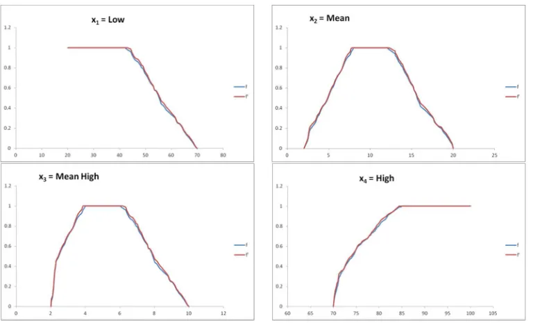
In Fig. 5 we show some FNs and their approximations obtained by applying the extended

320

F-transform. We set the threshold to 0.01, so having a RMSE less than 0.01 for every FN.

321

(15)

Fig. 5. Fuzzy numbers x1 = Low, x2 = Mean, x3 = Mean High and x4 = High (in blue) and their extended

323

iF-transform approximations (in red).

324

The FNs (x1 = Low) and (x4 = High) have a degenerated side. In Table 2.i we show the

325

parameters a, c, d, b of each FN xi (i = 1, 2, 3, 4, 5, 6 and the RMSE, respectively.

326

327

Table 2.1. Parameters and RMSE of the approximation for fuzzy sets of x1

328

x1 (m2) 

Fuzzy number

a c d b RMSE

Low 20 20 45 70 9.11×10-3

Mean Low 45 70 75 90 9.91×10-3

Mean 75 90 95 100 9.17×10-3

Mean High 95 100 115 125 9.76×10-3

High 110 120 150 150 9.34×10-3

329

330

x2

Fuzzy number a c d b RMSE

Low 0 0 1 4 9.18×10-3

Mean Low 0.5 3 6 8 9.43×10-3

Mean 2 7 12 20 9.19×10-3

Mean High 8 12 15 25 9.57×10-3

High 15 25 50 50 9.15×10-3

331

(16)

x3

Low 0 0 0.5 1 9.21×10-3

Mean Low 0.4 0.6 1 1.5 9.35×10-3

Mean 1 2 4 6 9.33×10-3

Mean High 2 4 7 10 9.02×10-3

High 6 10 30 30 9.26×10-3

333

334

x4

Low 0 0 30 40 9.24×10-3

Mean Low 30 50 60 70 9.29×10-3

Mean 60 65 70 80 9.49×10-3

Mean High 75 80 85 90 9.35×10-3

High 85 95 100 100 9.08×10-3

335

x5

Low 0 0 10 15 9.30×10-3

Mean Low 7 15 20 25 9.52×10-3

Mean 20 25 30 35 9.25×10-3

Mean High 30 35 40 50 9.31×10-3

High 40 50 100 100 9.37×10-3

336

337

x6

Low 0 0 10 15 9.32×10-3

Mean Low 7 15 25 30 9.19×10-3

Mean 22 28 32 35 9.24×10-3

Mean High 30 40 45 55 9.48×10-3

High 50 60 100 100 9.28×10-3

338

In Table 3 we show the parameter a, c, d, b of the FNs used for the output variable y and the

339

RMSE obtained applying the extended F-transform.

340

(17)

Table 3. Parameters and RMSE of the approximation for fuzzy sets of output y

342

y

Low 0 0 10 20 9.67×10-3

Mean Low 10 20 30 40 9.32×10-3

Mean 30 40 60 70 9.46×10-3

Mean High 50 70 80 85 9.78×10-3

High 80 90 100 100 9.31×10-3

343

At the end of the preprocessing phase, the fuzzification of the input data is performed as well.

344

In Figures 6i we show the thematic maps (in a Geographic Information System environment) of the

345

six input variables xi (i = 1,2, 3, 4, 5, 6), respectively, in the municipalities of the district of Naples. In

346

each map the municipality is classified with the linguistic label of the fuzzy set with the highest

347

approximated membership value.

348

349

Fig. 6.1. Thematic map for the input variable x1

350

351

Fig. 6.2. Thematic map for input variable x2

(18)

353

354

355

356

357

(19)

360

361

362

363

364

365

The defuzzified final values of liveability in the residential housings (calculated in percentage)

366

for every municipality are in Table 4.

367

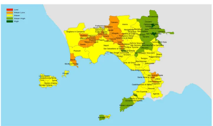
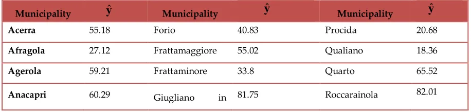
368

Table 4. Defuzzified values obtained for liveability of residential housings

369

Municipality Municipality Municipality

Acerra 55.18 Forio 40.83 Procida 20.68

Afragola 27.12 Frattamaggiore 55.02 Qualiano 18.36

Agerola 59.21 Frattaminore 33.8 Quarto 65.52

Anacapri 60.29 _Giugliano _{in 81.75} Roccarainola 82.01

ˆ

(20)

Campania

Arzano 23.34 Gragnano 29.64 SanGennaro Vesuviano

76.18

Bacoli 24.65 Grumo Nevano 55 SanGiorgio a Cremano

23.14

Barano d'Ischia 58.36 Ischia 27.13 SanGiuseppe Vesuviano

51.03

Boscoreale 32.23 Lacco Ameno 26.69 San Paolo BelSito 63.46

Boscotrecase 48.7 Lettere 42.57 San Sebastiano al Vesuvio

82.37

Brusciano 63.37 Liveri 81.39 San Vitaliano 66.52

Caivano 44.85 Marano di

Napoli 24.93

Santa Maria la Carità

56.94

Calvizzano 52.06 Mariglianella 82.39 Sant'Agnello 33.85 Camposano 50.84 Marigliano 53.68 Sant'Anastasia 64.19 Capri 47.32 Massa di Somma 36.15 Sant'Antimo 47.82 Carbonara di

Nola 73.29 MassaLubrense 71.5

Sant'Antonio Abate

58.19

Cardito 47.68 Melito di Napoli 26.87 Saviano 76.84 Casalnuovo di

Napoli 23.45 Meta 56.38 Scisciano

88.93

Casamarciano 92.74 Monte di Procida 32.69 Serrara Fontana 54.08 Casamicciola

Terme 34.61

Mugnano di

Napoli 29.14 Somma Vesuviana

52.11

Casandrino 39.26 Napoli 53.82 Sorrento 20.18

Casavatore 33.15 Nola 75.35 Striano 73.69

Casola di

Napoli 38.77 Ottaviano 52.94 Terzigno

52.01

Casoria 34.02 Palma Campania 62.9 Torre Annunziata 25.12 Castellammare

di Stabia 44.26 Piano di Sorrento 60.67 Torre del Greco

26.36

Castello di

Cisterna 73.89 Pimonte 27 Trecase

55.8

Cercola 49.67 Poggiomarino 75 Tufino 96.44

Cicciano 67.16 Pollena Trocchia 25.13 Vico Equense 20.37

Cimitile 87.38 Pomigliano

d'Arco 19.75 Villaricca

78.36

(21)

Crispano 39.07 Portici 22.51 Volla 55.83

Ercolano 28.14 Pozzuoli 39.43

370

In Fig. 7 we show a thematic map of the index of liveability in the residential housings: the label

371

of output variable fuzzy set with the greatest membership degree is assigned for every municipality.

372

373

374

Fig. 7. Thematic map of index of liveability in residential housings

375

376

We compare these results with the ones obtained by approximating the input and output

377

variables fuzzy sets with trapezoidal FNs, by using the approximation method of [20]. We apply the

378

inference system to the residential housing dataset again, by using the approximated trapezoidal

379

FNs as fuzzy sets in the antecedents and consequents of the rule set. Then we calculate the RMSE

380

and we calculate the number and the percentage of municipalities classified with a liveability

381

linguistic label different by the one contained in Fig.7.

382

383

Table 5. Comparisons obtained approximating input and output FN with trapezoidal FN

384

Comparison parameter Value

Mean RMSE index for the fuzzy sets approximation with

trapezoidal FNs

6.3×10-2

Mean difference of the final crisp liveability values compared with the ones obtained by using the extended iF-transform method

5.58%

Number of municipalities classified

with different linguistic labels 7

Percentage of municipalities classified with different linguistic

labels

(22)

385

The mean RMSE index obtained by using the trapezoidal FN is 6.3×10-2_{: this value is greater}

386

than the threshold 1×10-2 _{set by applying the extended F-transform. The mean difference in absolute}

387

value between the crisp liveability obtained by using the trapezoidal approximation of the input

388

and output FNs with respect to the ones obtained by using the extended IF-transform approximation

389

overcomes 5%: this difference is generated by the greater error obtained by the approximation with

390

trapezoidal FNs. The percentage 7.61% of the municipalities are classified differently in the final

391

map of liveability underlines the effective improvement of the final results obtained with the

392

extended F-transform method. The seven municipalities with different liveability class are given in

393

Table 6.

394

395

Table 6. Municipalities with different liveability class

396

Municipality Extended IFtr liveability class

Trapezoidal liveability class

Casola di Napoli Mean Mean Low

Casoria Mean Low Mean

Crispano Mean Mean Low

Massa di Somma Mean Mean Low

Pozzuoli Mean Mean Low

Sant’Agnello Mean Low Mean

Scisciano Mean High High

397

We can appropriately select the RMSE threshold in order to increase the reliability of the final

398

results, however we point out that that the choice of a very small threshold can lead to a fuzzy

399

uniform partition too finer for which the dataset of the corresponding values is not sufficiently

400

dense.

401

6. Conclusions

402

We present a new method based on the extended F-transform to approximate FNs. We apply

403

this method in a fuzzy rule-based system related to a spatial analysis problem consisting in the

404

evaluation of the liveability of residential housings in the municipality of the district of Naples. In

405

many spatial analysis problems, decision-making systems based on expert rules are used in order to

406

extract thematic maps of a final index. A finer approximation of the membership functions of the

407

fuzzy sets in the antecedents and in the consequents of the fuzzy rules is necessary to guarantee a

408

good reliability of the final thematic maps. In many cases, for example in participatory contexts in

409

which knowledge is provided by different experts, these FNs are assigned on a discrete set of points.

410

In future we propose to apply the extended F-transform method to the approximation of FNs in

411

multi-criteria fuzzy decision making problems.

412

413

Acknowledgments: This work is performed under the auspices of INDAM-GNCS (Gruppo Nazionale per il

414

Calcolo Scientifico), Italy.

415

416

Conflicts of Interest: The authors declare no conflict of interest with this research.

417

(23)

References

421

1. S. Abbasbandy, B. Asady, The nearest trapezoidal fuzzy number to a fuzzy quantity, Applied Mathematics and

422

Computation 156 (2) (2004) 381–386. Doi: 10.1016/j.amc.2003.07.025

423

2. S. Abbasbandy, T. Hjjari, Weighted trapezoidal approximation–preserving cores of a fuzzy number, Computer

424

and Mathematics with Applications 59 (2010) 3066–3077. Doi: 10.1016/j.camwa.2010.02.026

425

3. A.I. Ban, L. Coroianu, Nearest interval, triangular and trapezoidal approximation of fuzzy number preserving

426

ambiguity, International journal of Approximate Reasoning 53 (2012) 805–836.

427

Doi:10.1016/j.ijar.2012.02.001

428

4. A.I. Ban, Approximation of fuzzy numbers by trapezoidal fuzzy numbers preserving the expected interval, Fuzzy

429

Sets and Systems 159 (2008) 1327–1344. Doi:10.1016/j.fss.2007.09.008

430

5. L. Coroianu, Lipschitz functions and fuzzy number approximations, Fuzzy Sets and Systems 200 (2012)

431

113–135. Doi: 10.1016/j.fss.2012.01.001

432

6. L. Coroianu, M. Gagolewski, P. Grzegorzewski, Nearest piecewise linear approximation of fuzzy numbers,

433

Fuzzy Sets and Systems 233 (2013) 26–51. Doi:10.1016/j.fss.2013.02.005

434

7. L. Coroianu, S. G. Gal, B. Bede, Approximation of fuzzy numbers by Bernstein operators of max–min product

435

kind, Fuzzy Sets and Systems 257 (2014) 41–66. Doi: 10.1016/j.fss.2013.04.010

436

8. L. Coroianu, L. Stefanini, General approximation of fuzzy numbers by F–transform, Fuzzy Sets and Systems 288

437

(2016) 46–74. Doi: 10.1016/j.fss.2015.03.015

438

9. M. Delgado, M.A.Vila, W.Voxman, On a Canonical Representation of a Fuzzy number, Fuzzy Sets and Systems

439

93 (1998) 125–135.Doi: 10.1016/S01650114(96)001443

440

10. F. Di Martino, V. Loia, I. Perfilieva, S. Sessa, An image coding/decoding method based on direct and inverse fuzzy

441

transforms, International Journal of Approximate Reasoning 48 (1) (2008) 110–131.

442

Doi:10.1016/j.ijar.2007.06.008

443

11. F. Di Martino, V. Loia, S. Sessa, Fuzzy transforms method and attribute dependency in data analysis, Information

444

Sciences 180 (4) (2010) 493–505. Doi: 10.1016/j.ins.2009.10.012

445

12. F. Di Martino, V. Loia, S. Sessa, Fuzzy transforms method in prediction data analysis, Fuzzy Sets and Systems

446

180 (1) (2011) 146–163. Doi:10.1016/j.fss.2010.11.009

447

13. F. Di Martino, P. Hurtik, I. Perfilieva, S. Sessa, A color image reduction based on fuzzy transforms, Information

448

Sciences 266 (4) (2014) 101–111. Doi:10.1016/j.ins.2014.01.014

449

14. F. Di Martino, S. Sessa, Complete image fusion method based on fuzzy transforms, Soft Computing (2017) 1–11.

450

Doi: 10.1007/s00500.

451

15. F. Di Martino, S. Sessa, Fuzzy transforms prediction in spatial analysis and its application to demographic balance

452

data, Soft Computing 21 (13) (2017) 3537–3550. Doi:10.1007/s0050001726218

453

16. D. Dubois, H. Prade, Operations on fuzzy numbers, Ins. J. Systems Sci. 9 (1978) 613–626. Doi:

454

10.1080/00207727808941724

455

17. P.Grzegorzewski, Metrics and Orders in Space of Fuzzy Numbers, Fuzzy Sets and Systems 97 (1998) 83–94.

456

Doi: 10.1016/S01650114(96)003223

457

18. P. Grzegorzewski, Nearest interval approximation of a fuzzy number, Fuzzy Sets and Systems 130 (2002)

458

321–330. Doi:10.1016/S01650114(02)000982

459

19. P. Grzegorzewski, E. Mrówka, Trapezoidal approximations of fuzzy numbers, Fuzzy Sets and Systems 153

460

(2005) 115–135. Doi: 10.1016/j.fss.2004.02.015

461

20. P. Grzegorzewski, Trapezoidal approximations of fuzzy numbers preserving the expected interval—Algorithms and

462

properties, Fuzzy Sets and Systems 159 (2008) 1354–1364. Doi: 10.1016/j.fss.2007.12.001

463

21. S. Heilpern, The expected value of a fuzzy number, Fuzzy Sets and Systems 47 (1992) 81–86. Doi:

464

10.1016/01650114(92)900629

465

22. E. H. Mamdani, Application of fuzzy logic to approximate reasoning using linguistic synthesis. IEEE Transactions

466

on Computers 26 (12) (1977) 1182–1191.Doi: 10.1109/TC.1977.1674779

467

23. E. N. Nasibov, S. Peker, On the nearest parametric approximation of a fuzzy number,Fuzzy Sets and Systems

468

159 (11) (2008) 1365–1375. Doi:10.1016/j.fss.2007.08.005

469

24. I. Perfilieva, Fuzzy transforms: theory and applications, Fuzzy Sets and Systems 157 (2006) 993–1023. Doi:

470

10.1016/j.fss.2005.11.012

471

25. I. Perfilieva, V. Novak, A. Dvorak, Fuzzy transforms in the analysis of data, International Journal of

472

(24)

26. I. . Perfilieva, P. Hurtík, F. Di Martino, S. Sessa, Image reduction method based on the F–transform, Soft

474

Computing 21(7) (2017) 1847–1861.Doi: 10.1007/s0050

475

27. I. Perfilieva, B. De Baets, Fuzzy transforms of monotone functions with application to image compression,

476

Information Sciences 180 (17) (2010) 3304–3315. Doi: 10.1016/j.ins.2010.04.029

477

28. L. Stefanini, L. Sorini, Type–2 fuzzy numbers and operations by F–transform, IFSA World Congress and

478

NAFIPS Annual Meeting (IFSA/NAFIPS), 24–28/06/2013, pp. 1050–1055. Doi:

479

10.1109/IFSA–NAFIPS.2013.6608545

480

29. C-T. Yeh, Weighted semi–trapezoidal approximations of fuzzy numbers, Fuzzy Sets and Systems, 165 (2011)

481

61–80. Doi: 10.1016/j.fss.2010.11.001

482

30. C-T. Yeh, Existence of interval, triangular, and trapezoidal approximations of fuzzy numbers under a general

483

condition, Fuzzy Sets and Systems 310 (2017) 1–13. Doi: 10.1016/j.fss.2016.03.013

484

31. W. Zeng, H. Li, Weighted triangular approximation of fuzzy numbers, International Journal of Approximate

485

Reasoning 46 (2007) 137–150. Doi: 10.1016/j.ijar.2006.11.001