A Particle Swarm Optimization based
Machine Learning Approach for Wave Height
Prediction
Neha Sharma1, Pranita Jain2
M. Tech Scholar, Department of Computer Science and Engineering, SATI, Vidisha, India1
Assistant Professor, Department of Computer Science and Engineering, SATI, Vidisha, India2
ABSTRACT: The prediction of wave height is one of the major problems of coastal engineering and coastal structures. In recent years, advances in the prediction of significant wave height have been considerably developed using flexible calculation techniques. In addition to the traditional prediction of significant wave height, soft computing has explored a new way of predicting significant wave heights. This research was conducted in the direction of forecasting a significant wave height using machine learning approaches.In this paper, a problem of significant wave height prediction problem has been tackled by using wave parameters such as wave spectral density. This prediction of significant wave height helps in wave energy converters as well as in ship navigation system. This research will optimize wave parameters for a fast and efficient wave height prediction. For this Particle Swarm Optimization feature reduction techniques are used. So reduced features are taken into consideration for prediction of wave height using neural network, extreme learning machine random forest forecasting and support vector machine forecasting technique. In this work, performance evaluation metrics such as MSE RMSE and MAE values are decreased and gives better performance of classification that is compared with existing research’s implemented methodology. From the experimental results, it is observed that proposed algorithm gives the better prediction results with PSO feature reduction technique and ELM forecasting techniques and achieved about 0.25 RMSE as well as 0.24 MAE.
KEYWORDS: Machine Learning, Wave height Prediction, Correlation Co-efficient, Accuracy.
I. INTRODUCTION
Wave energy transfer provides a convenient and natural concentration of wind energy within the waves.Wave energy generation refers to the energy ofocean surface waves and the utilization of that energy to generateelectricity. The energy within a wave is dependent on the followingfactors; wind speed, duration of the wind blowing, the distanceof open water that the wind has blown over (fetch), andwater depth [1]. Wave power could be determined by wave height, wavelength, and water density. This mathematically could be described as in [2]:
=
64 ≈
1
2 /
Where, P is the wave energy flux per unit wave crest length (kW/m);q the mass density of the water (kg/m3); g the gravitational gravity(m/s2); H the wave height (m) and T is the wave time cycle (s).For example: for a 1.6 m wave and 10 s period, the power producedis approximately 12.8 kW/m.
Ocean waves’ kinetic energy can be transformed into electricity by means of Wave Energy Converters (WEC), contributing this way to reduce our deep dependence on fossil fuels [3]. This type of marine facilities to obtain energy shows a clear potential for sustainable growth [4]: marine energy resources do not generate CO2 and reduce oil imports, a crucial geo-economical issue.
converters, their related economical aspects, and the potential of a number of ocean regions to be exploited worldwide) can be found in [6]. Ocean waves are usually produced by wind action and are therefore an indirect form of solar energy. Wave energy uses Wave Energy Converters (WECs) to convert ocean energy into electricity.
WECs transform the kinetic energy of wind-generated waves into electricity by means of either the vertical oscillation of waves or the linear motion of waves, and exhibit some important advantages when compared to alternatives based on tidal converters, for example. Note however, that not all of the available wave energy resources can be realized as usable power, mainly due to various factors including socio-economics, the severe ocean environment, power conversion losses, and cost. Moreover, ocean waves are difficult to characterize, because its generation and propagation can be modelled as nonlinear processes. The real sea is a superposition of irregular waves trains which differ in period, height and direction. The local behaviour of the sea estate can be represented by a spectrum, which specifies how the wave energy is distributed in terms of frequency and direction. As a consequence of this complexity, both the design, deployment, and control of WECs [7],become key topics that require a proper characterization and prediction of waves. Maybe, the most important wave parameters in this regard to characterize waves is the significant wave height (Hs), in which prediction this paper is focused on.
Wave height is one of the most important factors in coastal processes and coastal engineering studies is discussed by DevanshuKanojiya in [9]. In case of energy extraction from waves, sediment movements, harbour design and soil erosion, wave height plays a vital role in these. Long- term observed data are needed for all the practical applications. There are different methods for finding wave heights such as field measurements, theoretical studies and numerical stimulation [9]. But in most of these cases there won’t be long-term measurements, so prediction of wave height is essential. Now day’s soft computing-based models have been used for wave prediction.
Soft computing based methods give results with high accuracy and time taken for training and prediction is very less compared to other traditional methods [10,11].
As mentioned above, the stochastic nature of the waves makes it very difficult to predict the wave energy resource, so research on this topic has been intense in recent years. From the point of view of machine learning approaches, one of the first wave height prediction algorithms proposed using artificial neural networks is used to obtain an accurate prediction of wave height. Alternative proposals based on different approaches have been recently proposed, with various soft calculation techniques being tested for wave height prediction [12-15].
The objective of this research is to maximize the prediction speed of wave height by minimizing and selecting the optimal properties. Weather forecasts and energy production will benefit from the assessment of wave height with emphasis on the characteristics that result from this analysis.
II. RELATED WORK
An artificial neural network was used by Deo and Chaudhari (1998) [1] to predict the tides on both coasts of India. From monthly data on average wave height, Deo and Kumar (2000) [3] obtained weekly wave height data. Backpropagation has been implemented by Mandal (2001) [2] for tide forecasting.
A three-layer feedforward artificial neural network has been described by Deo et al. (2001) [4] for the prediction of wave height and average wave period of three hour values. The current wind speed and the previous one-stage wind speed were used as inputs. For data at short intervals, he trained separately for the monsoon and post-monsoon weather conditions. Furthermore, they conclude that sampling and wind duration do not play an important role as input into neural networks.
Makarynskyy (2004) [5] used the artificial neural network to predict significant wave heights and wavelengths equal to zero crossing for a time interval of 1 hour to 24 hours. It also increased predictive accuracy by combining data from neural networks. The forward-back propagation method and the radial polarization function have been described by Kalra et al. (2005) [6] for the prediction of a significant wave height. The wind speed, the significant wave height and the average wave period were provided as input.
The wave period and the wave height generated by the cyclone were observed by Rao and Mandal (2005) [7] using two input configurations in ANN. The speed of the direct cyclone, the maximum radius of the wind speed and the central pressure were used as input in the first configuration, while the wind speed and the return were used as input for the second configuration.
The result shows that ANN shows the best result with all input parameters. In these input parameters, the wind speed has the maximum effect on the height of the output shaft.
Özger (2009) [9] used the neuro-fuzzy hybrid approach to estimate the characteristics of ocean waves. To overcome the problem of missing data, shows that the significant wave. The altitude of a boa position can be predicted using data from adjacent buoys using the neuro fuzzy approach. This approach shows a way to interrogate the lack and also to determine the optimal position of the buoys.
Salcedo. to the. (2014) [20] used the fuzzy inference system to predict wave parameters. They used length, duration, wind speed and wave height as variables to predict wave height and used various combinations. They compared their results with JONSWAP, EMC, Wilson, PMS and found that ANFIS is the best model with fewer errors. They also found that the combination of wind speed and blown wind duration as input gives a better result.
Hashimet. to the. (2016) [15] the selection of climate parameters using an improved Takagi-Sugeno blurring that influences the prediction of wave height. They used wind speed, wind direction, sea surface temperature and air temperature as input and significant wave height as a reference. The main objective of this study was to determine the main input parameters that influence wave height prediction. They found that wind speed, air temperature, sea surface temperature and wind direction have the least impact on wave prediction. They also found that the combination of wind speed, air temperature and wind direction are the most influential parameters [17,18].
Stefanakos (2016) [21] predicted non-stationary wind and wave data using fuzzy type Inference system (FIS) and Inference system blur based on an adaptive matrix (ANFIS) removes the non-stationary wind wave data before expected data. Data is first multiplied by the non-stationary modelling above in a residual and seasonal time series with a seasonal standard deviation removed and applied to a FIS or ANFIS model. With this method, they obtained a one-off forecast for specific data points and a field for prediction field for the whole wave parameter field [19,20]. The results were compared only with FIS and ANFIS and show that the combination goes beyond these methods.
III.PROPOSED METHODOLOGY
In the current scenario, an algorithm is proposed which provide a way to predict the significant wave height.Figure 1 shows the location of five buoy location i.e. “42056”, “42057”, “42058”, “42059” and “42060” taken from National Oceanic and Atmospheric Administration (NOAA) [16]. This research work is intended to predict the significant wave height at 42058 buoy center.The yellow dots represents the buoy location. The wave describing parameters have been formally computed on the basis of spectral wave density measured hourly by NOAA at each buoy centers during 2017.
Figure 1: Map Representation of Buoy Location in Caribbean Sea A. Wave Parameters
As mentioned above based on the hourly wave spectral density data collected at five different buoys, following 15 wave parameters are calculated in order to predict significant wave height. The main wave parameters are [21,22]: Wave Spectral Moments
= ∗ ( ) (1)
Where S(f) is the spectral density data from given buoy and n=-1, 0, 1, 2………..
They provide information on different statistical and physical characteristics of waves. For instance, m0 is the variance of the wave elevation.
Wave Height
The significant wave height is calculated as :
= 4( ) (2)
Hs the parameter related to the wave height that is most used in wave energy and in the design of ships and marine structures and coastal protection.
Peak Period
The peak period is defined as:
= 1 (3)
fp is the maximum spectral peak frequency. Wave Mean Period
It can be computed by using, among others, the estimator Txy as:
= (4)
Txy is an estimate of the average period used in the design of turbines for wave energy conversion. In this research work Tm01, Tm02, Tm-10 are calculated.
Goda'sPeakedness Parameter It is computed as:
= 2 . ( ) (5)
Qp has the potential to describe the statistical features of consecutive wave heights. Longuet–Higgins Spectral Bandwidth
It is computed as:
= ∗ −1 (6)
Quantifies the degree to which spectral energy spreads over the frequency range.
Wave Height Correlation Coefficient It is computed as:
=ℇ( )−
( )
−
1− (7)
Where k, parameter which is calculated as:
= | 1 ( )∗ | (8)
Particle Swarm Optimization Feature Reduction The basic process of the PSO algorithm is given by:
Step 1: (Initialization) Randomly generate initial particles. For the PSO algorithm, the complete set of features is represented by a string of length N.
Step 2: (Fitness) Measure the fitness of each particle in the population. The selection of this fitness function is a crucial point in using the PSO algorithm, which determines what a PSO should optimize. Here, the task of the PSO algorithm is to find the global minimum value according to the definition of the fitness function. The definition of the fitness function for the basic method is simply the accuracy of detection.
Step 3: (Update) Compute the velocity of each particle.
Step 4: (Construction) For each particle, move to the next position.
Step 5: (Termination) Stop the algorithm if the termination criterion is satisfied; return to Step 2 otherwise.
B. Proposed Methodology
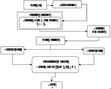
The proposed model is designed to predict the wave height at buoy location 42058 by analysing the significant wave features at four different buoy locations i.e. 42056, 42057, 42059, and 42060. To predict the significant wave height at particular location proposed algorithm flow chart is shown in figure 2.
The proposed algorithm is divided into three sections i.e. data collection and preprocessing, feature reduction and finally forecasting using neural network. In first stage the real time data is collected from National Oceanic and Atmospheric Administration (NOAA) for five different buoy centres which is discussed above. Further the data is used to extract 15 different features using wave parameters. And further the extracted features are reduced by using co-relation analysis which determines that which wave parameters are more efficient to determine the significant wave height.And in last step neural network is used to forecast the wave height at buoy location 42058 in jan-feb 2018.
Figure 2:Flow Diagram of Proposed Methodology for Wave Height Prediction Preprocessing
Data Set
Feature Selection
Particle Swarm Optimization (PSO)
Reduced Dimension
Data Splitting
Testing Data Training Data
Result
Forecasting Methods
C. Forecasting Methods Neural Network Forecasting
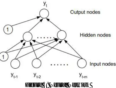
Neural networks are a class of nonlinear flexible models that can adaptively recognize models from data. In theory, it has been shown that neural networks can learn from experience in an appropriate number of nonlinear processing units and can estimate any complex functional relationship with great accuracy. Empirically, many successful applications have established their role in pattern recognition and prediction. Although many types of neural network models have been proposed, the most common model for time series prediction is the direct acting network model. Figure 3.3 shows a typical three-layer feedforward model used for prediction purposes. The input nodes are the previous delayed observations, while the output provides the forecast for the future value.
Figure 3: Neural Network
Hidden nodes with appropriate non-linear transfer functions are used to process the information received from the input nodes. The model can be written as:
= + ( + ) + (9)
where m is the number of input nodes, n is the number of hidden nodes, f is a sigmoid transfer function, such as logistics:
( ) = 1
1 + exp(− )∗{ , = 0,1,2, … … . , } (10)
is a vector of weights from the hidden to output nodes and {βij ,i=0,1, ... , m; j =1,2,….,n} are the weights of the input
to the hidden nodes α0 and β0j the weights of the arcs resulting from the polarization terms whose values are always equal to 1. It should be noted that the linear transfer function it is used in the root node as desired for forecasting problems.
Extreme Learning Machine Forecasting
The single-hidden layer-feed-forward neural network – also termed as ELM – an learn exactly N different observations on almost all non-linear activation functions with at most N hidden nodes. The main difference between ELM and the traditional formation of an electric network is that the hidden ELM layer does not need a setting that randomly selects hidden level parameters. Input weights, hidden neural bias, and hidden layer output weights are randomly assigned to minimize drive failure. ELM transforms the learning problem into a simple linear system in which the initial weights can be determined analytically. For N arbitrary distinct instances {(xi, yi),i = 1, 2, . . . , N}, where xiandyiELM with n inputs, m outputs, k hidden neurons, and an activation function g(x) is modelled as:
Where wiand βirepresent the weight vectors connecting the input neurons to an ith hidden neurons to the output neurons, respectively, and bi is a threshold of the ith hidden neurons. The ELM with k = N hidden neurons can reliably approximate these N instances with zero error as
| − | = 0 (12)
( + ) = , = 1,2,3, … … . . (13)
The matrix y is the ELM hidden layer output matrix, in which the i-th column of y is the output of the hidden neuron
with respect to the inputs x1, x2. ,,, xN. In the basic ELM, if k << N and Υ are a non-square matrix, learning the ELM
is equivalent to finding a solution of the least squares β of the linear system Yβ = T.
Decision Tree Forecasting
The decision model is based on the actual values of the attributes in the data. The decision interval continues until a prediction decision is made for a given record. It has a default destination variable. Decision trees are trained in the data for classification and regression problems. Decision trees are popular in machine learning because they are often quick and precise. It works for categorical and continuous input and output variables. In this technique, the population or sample is divided into two or more homogeneous subpopulations or more based on the most significant fragment in the input variables.
The decision is taken from the tree in the strategic division. This greatly affects the accuracy of the tree. This decision criterion differs for classification and regression trees in Figure 3.4. Decision trees use different algorithms to decide to divide a node into two or more subnodes. The trees break the nodes for all the available variables, then select the division that leads to the most homogeneous sub-nodes. The most popular decision tree algorithms are: Random Forest and least square boosting(LSBoost).
Gaussian Kernel based Support Vector Machine (SVM)
This is for classification and regression problems. SVM classifies data into different classes by identifying a hyperplan (line) that separates learning data into classes. The hyperplane's identification, which maximizes the distance between classes, increases the probability of generalizing secret data. SVM offers the best classification performance i.e. the accuracy of the training set. It does not overflow the data.
SVM does not make strong assumptions about the data. Show more efficiency in the correct classification of future data. SVM is classified into two categories, i.e. Linear and non-linear. In a linear approach, training data is represented by a line, i.e. hyperplane, shown separately.
Consider the problem of separating the set of training vectors belonging to two distinct classes, G = {(xi; yi); i = 1; 2;:::;N} with a
hyperplane wT*(x) + b =0 (xi is the ith input vector, yi∈ {−1; 1} is known binary target), the original SVM classi1er
satisfies the following conditions:
wT*ϕ(xi) + b≥ 1 if yi= 1 wT*ϕ(xi) + b≤1 if yi= -1
(14)
where ϕ: Rn→ Rm is the feature map mapping the input space to a usually high dimensional feature space where the data points become linearly separable.
The distance of a point xi from the hyperplane is
( , , ) =| ∗ ∅( ) + |
| | (15)
∅( ) =1
2| | (16)
For the inseparable linear problem, we first assign the data to another large space using a non-linear mapping, which
we call Φ. So we use the linear model to achieve classification in new space . Through defined “kernel function” , is converted as follows:
−1
2 ( ⃗ ∗ ⃗)
,
(17)
. .∑ = 0 0≤ai≤C, i=1,2,………l (18) And corresponding classification decision function is converted as follows:
( ) = [ ( ⃗ ∗ ⃗) + ] (19)
The selection of kernel function aims to take the place of inner product of basic function. The kernel function investigates the non-separable problems as follows:
= exp(− | − | (20)
IV.RESULT ANALYSIS
A. Dataset Description
A news dataset from National Oceanic and Atmospheric Administration (NOAA) is prepared for this research work. The data is collected from buoy centers from Caribbean Sea. The location of five buoy location i.e. “42056”, “42057”, “42058”, “42059” and “42060” taken from National Oceanic and Atmospheric Administration (NOAA). This research work is intended to predict the significant wave height at 42058 buoy centres.
B. Performance Parameters Mean Square Error (MSE)
MSE of any estimator (classifier) measures the average squares of errors or deviations, i,e. the difference between the estimator and what is estimated. MSE is a risk function corresponding to the expected value of the squared error loss.
= 1( − ) (21)
Root Mean Square Error (RMSE)
RMSE is a parameter that determines the difference in squares between the output and the input.
=√ (22)
Mean Absolute Error (MAE)
MAE measures the average size of errors in a series of forecasts regardless of their direction. This is the average of absolute differences between prediction and actual observation, in which all individual differences are also weighted.
=1 − (23)
As mentioned before, the evaluation parameters are mean square error (MSE) as well as root mean square error (RMSE) and mean absolute error (MAE). In this proposed algorithm the feature optimization or reduction technique is used with neural network, extreme learning technique, support vector regression and random forest decision tree regression are applied on dataset. The result analysis describes that out of 15 parameters only seven parameters are co-related i.e. which have impact on deciding significant wave height of the waves.
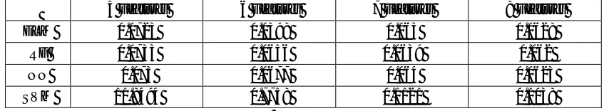
Table I: Performance Analysis of MSE, RMSE and MAE for Wave Height Prediction Techniques MSE
5 Features 6 Features 7 Features 8 Features
ELM 0.0723 0.0598 0.063 0.0628
RF 0.0733 0.0656 0.0639 0.062
NN 0.073 0.0677 0.064 0.0623
SVM 11.8494 0.7758 0.1121 0.1038
RMSE
5 Features 6 Features 7 Features 8 Features
ELM 0.2688 0.2445 0.251 0.2505
RF 0.2708 0.2561 0.2528 0.249
NN 0.2703 0.2602 0.2529 0.2496
SVM 3.4423 0.8808 0.3348 0.3222
MAE
5 Features 6 Features 7 Features 8 Features
ELM 0.2687 0.2424 0.2492 0.2489
RF 0.2707 0.2546 0.2503 0.2466
NN 0.2702 0.2544 0.2503 0.2471
SVM 3.4423 0.8808 0.3348 0.3222
Figure 4: Comparative Analysis of MSE
Figure 5 represents the performance of ELM, NN and RF algorithms with respect to RMSE. The simulation result are carried out for 5, 6, 7 and 8 Features. After selecting efficient feature from the wave parameters, it has been analyzed by increasing number of features and calculated the MSE. From the figure 4 it has been noted that MSE is least 6 features using ELM technique.
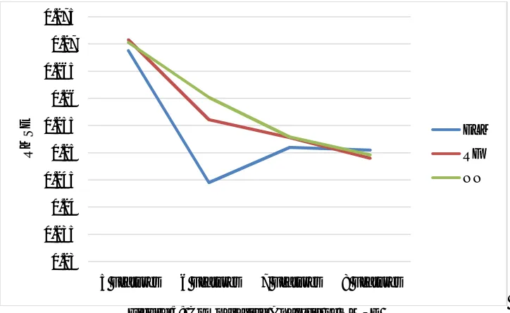
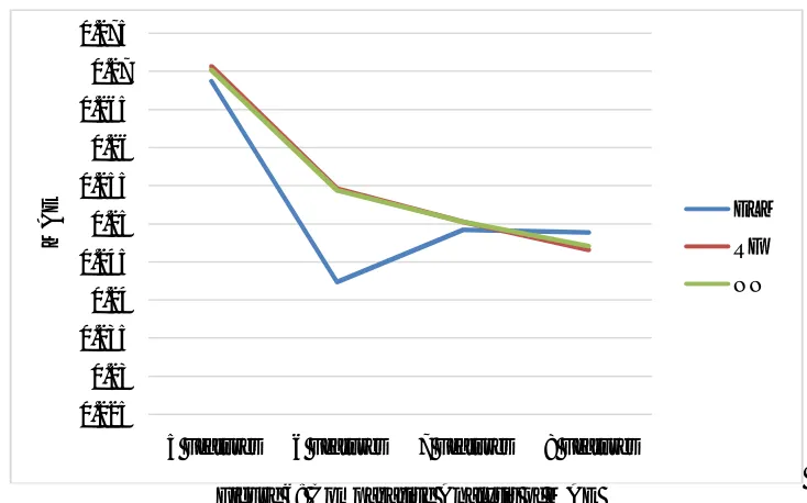
Figure 5: Comparative Analysis of RMSE
Figure 5 represents the performance of ELM, NN and RF algorithms with respect to RMSE. The simulation result are carried out for 5, 6, 7 and 8 Features. After selecting efficient feature from the wave parameters, it has been analyzed by increasing number of features and calculated the RMSE. From the figure 5 it has been noted that RMSE is least 6 features by using ELM technique.
0 0.01 0.02 0.03 0.04 0.05 0.06 0.07 0.08
5 Features 6 Features 7 Features 8 Features
M
S
E ELM
RF
NN
0.23 0.235 0.24 0.245 0.25 0.255 0.26 0.265 0.27 0.275
5 Features 6 Features 7 Features 8 Features
R
M
S
E ELM
RF
Figure 6: Comparative Analysis of MAE
Figure 6 represents the performance of ELM, NN and RF algorithms with respect to MAE. The simulation result are carried out for 5, 6, 7 and 8 Features. After selecting efficient feature from the wave parameters, it has been analyzed by increasing number of features and calculated the MAE. From the figure 6 it has been noted that MAE is least 6 features by using ELM technique.
After analysing the two feature reduction techniques with different forecasting techniquesbest results are given as: i. Minimum MSE is achieved by using ELM Technique which is approximately equal to 0.06 while using 6
features.
ii. Minimum RMSE is achieved by using ELM Technique which is approximately equal to 0.25 while using 6 features.
iii. Minimum MAE is achieved by using ELM Technique which is approximately equal to 0.245 while using 6 features.
V. CONCLUSION
Ocean energy is clean and renewable but has less environmental reserves. In this work, the use of artificial intelligence (AI) in the field of wave height prediction is studied. The advantages of applying AI techniques to energy problems are their great potential to handle a plethora of inaccurate or missing data. The research focused on the use of machine learning techniques to predict significant wave heights. The predictive power of a machine learning approach depends on the quality and size of all available data. Hybrid models offer better results than simple models. wind speed, air temperature, sea surface temperature and wind direction with minimal impact on wave height prediction. The combination of wind speed, air temperature and wind direction is all the most influential input parameters.
In this research, a problem of the prediction problem of the height of significant waves was solved using wave parameters such as wave spectral density. This significant wave height prediction helps both wave power converters and onboard navigation systems. This research will optimize wave parameters for a fast and efficient wave height prediction. For this Particle Swarm Optimization feature reduction techniques are used. So reduced features are taken into consideration for prediction of wave height using neural network, extreme learning machine random forest forecasting and support vector machine forecasting technique. In this work, performance evaluation metrics such as MSE RMSE and MAE values are decreased and gives better performance of classification that is compared with existing research’s implemented methodology. From the experimental results, it is observed that proposed algorithm gives the better prediction results with PSO feature reduction technique and ELM forecasting techniques.The future
0.225 0.23 0.235 0.24 0.245 0.25 0.255 0.26 0.265 0.27 0.275
5 Features 6 Features 7 Features 8 Features
M
A
E ELM
RF
work will be intended to predict some other wave parameters as well as may be applied in order to predict the amount of energy generated by waves at buoy centres.
REFERENCES
[1] Deo, M.C Chaudhari, G., 1998. Tide prediction using neural networks. Computer Aided Civil and Infrastructure Engineering 13, 113–120.
[2] Mandal, S., 2001. Back propagation neural network in tidal level forecasting. Journal of Waterway, Port, Coastal and Ocean Engineering 127 (1), 54–55. [3] Deo, N.C., Kumar, N.K., 2000. Interpolation of wave heights. Ocean Engineering 27, 907–919.
[4] Deo, M.C., Jha, A., Chaphekar, A.S., Ravikant, K., 2001. Neural networks for wave forecasting. Ocean Engineering 28, 889–898 [5] Makarynskyy, O., 2004. Improving wave predictions with artificial neural networks. Ocean Engineering 31 (5–6), 709–724
[6] Kalra, R., Deo, M.C., Kumar, R., Aggarwal, V.K., 2005a. Artificial neural network to translate offshore satellite wave data to coastal locations. Ocean Engineering 32, 1917–1932
[7] Rao, S., Mandal, S., 2005. Hindcasting of storm waves using neural networks. Ocean Engineering 32, 667–684.
[8] Kemal Gunaydın, 2008. The estimation of monthly mean significant wave heights by using artificial neural network and regression methods. Ocean Engineering 35 (2008) 1406–1415.
[9] Mehmet Özger, 2009. Neuro-fuzzy approach for the spatial estimation of ocean wave characteristics. Advances in Engineering Software 40 (2009) 759– 765
[10] AdemAkpınar , Mehmet O¨ zger, Murat I˙hsanKo¨mu¨rcu, 2014. Prediction of wave parameters by using fuzzy inference system and the parametric models along the south coasts of the Black Sea. J Mar SciTechnol (2014) 19:1–14DOI 10.1007/s00773-013-0226-1.
[11] S. Salcedo-Sanza,n, J.C.NietoBorge, L.Carro-Calvo a, L.Cuadra a, K.Hessner b, E. Alexandre, 2015. Significant wave height estimation using SVR algorithms and shadowing information from simulated and real measured X-band radar images of the sea surface. Ocean Engineering101(2015)244–253. [12] J.C. Fernández a, S. Salcedo-Sanzb,n, P.A. Gutiérrez a, E. Alexandre b, C. Hervás-Martínez, 2015. Significant wave height and energy flux range
forecast with machine learning classifiers. Engineering Applications of Artificial Intelligence 43 (2015) 44–53.
[13] L. Cornejo-Bueno, J.C. Nieto Borgea, E. Alexandre, K. Hessner, S. Salcedo-Sanz, 2016. Accurate estimation of significant wave height with Support Vector Regression algorithms and marine radar images. Coastal Engineering 114 (2016) 233–243.
[14] L. Cornejo-Bueno a, J.C. Nieto-Borge a, P. García-Díaz a, G. Rodríguez b, S. Salcedo-Sanz, 2016. Significant wave height and energy flux prediction for marine energy applications: A grouping genetic algorithm e Extreme Learning Machine approach. Renewable Energy 97 (2016) 380e389.
[15] RoslanHashima, Chandrabhushan Roy, Shervin Motamedia, ShahaboddinShamshirband, DaliborPetković , 2016. Selection of climatic parameters affecting wave height prediction using an enhanced Takagi-Sugeno-based fuzzy methodology. Renewable and Sustainable Energy Reviews 60(2016)246–257.
[16] http://www.ndbc.noaa.gov/
[17] DevanshuKanojiya, Dr. Manish Khemariya, “A Review on Ocean Energy Power Generation Technologies”, IJOSCIENCE, Volume III, Issue VI July 2017.
[18] PradnyaDixita, ShreenivasLondhe, 2016. Apor Prediction of extreme wave heights using neuro wavelet technique. Applied Ocean Research 58 (2016) 241–252.
[19] S. Salcedo-Sanza,n, J.C.NietoBorge, L.Carro-Calvo a, L.Cuadra a, K.Hessner b, E. Alexandre, 2015. Significant wave height estimation using SVR algorithms and shadowing information from simulated and real measured X-band radar images of the sea surface. Ocean Engineering101(2015)244–253. [20] Christos Stefanakos, 2016. Fuzzy time series forecasting of nonstationary wind and wave data. Ocean Engineering121(2016)1–12.
[21] PradnyaDixita, ShreenivasLondhe, 2016. Apor Prediction of extreme wave heights using neuro wavelet technique. Applied Ocean Research 58 (2016) 241–252.
[22] E. Alexandre, L. Cuadra, J.C. Nieto-Borge, G. Candil-García, M. del Pino, S. Salcedo-Sanz, “A hybrid genetic algorithm—extreme learning machine approach for accurate significant wave height reconstruction”, Elsevier, (2015).
[23] Ozger, M., Sen, Z., 2007. Prediction of wave parameters by using fuzzy logic approach. Ocean Eng. 34, 460–469
[24] M.H. Moeini, Etemad-Shahidi, 2007. Application of two numerical models for wave hindcasting in Lake Erie. Applied Ocean Research 29 (2007) 137– 145
[25] Mahjoobi J, Etemad-Shahidi, Kazeminezhad, M.H., 2008. Hindcasting of wave parameters using different soft computing methods. Appl. Ocean Res. 30, 28–36
[26] Mahjoobi J, Etemad-Shahidi, 2008. An alternative approach for prediction of significant wave height based on classification and regression trees. Applied Ocean Research, Accepted
[27] Surabhi Gaur, M.C. Deo, 2008. Real-time wave forecasting using genetic programming. Ocean Engineering 35 (2008) 1166– 1172.
[28] Kemal Gunaydın, 2008. The estimation of monthly mean significant wave heights by using artificial neural network and regression methods. Ocean Engineering 35 (2008) 1406–1415
[29] J. Mahjoobi, EhsanAdeli Mosabbeb,2009. Prediction of significant wave height using regressive support vector machines. Ocean Engineering 36 (2009) 339–347.
[30] Mehmet Özger, 2009. Neuro-fuzzy approach for the spatial estimation of ocean wave characteristics. Advances in Engineering Software 40 (2009) 759– 765
[31] GeorgiosSylaios, Frederic Bouchette, Vassilios.Tsihrintzis ,CleaDenamiel, 2009. A fuzzy inference system for wind-wave modeling. Ocean Engineering 36 (2009) 1358–136.
[32] MortezaZanaganeh a, S.JamshidMousavi b, AmirFarshadEtemadShahidi, 2009. A hybrid genetic algorithm–adaptive network-based fuzzy inference system in prediction of wave parameters. Engineering Applications of Artificial Intelligence 22 (2009) 1194–1202.
[33] A. Etemad-Shahidi, J. Mahjoobi, 2009. Comparison between M5’model tree and neural networks for prediction of significant wave height in Lake Superior. Ocean Engineering 36 (2009) 1175–1181
[34] B. Can˜ellas, S.Balle,J.Tintore´ ,A.Orfila, 2010. Wave height prediction in the Western Mediterranean using genetic algorithms. Ocean Engineering 37 (2010) 742–748