Crime Patterns and Prediction: A Data Mining and Machine Learning Approach

(1)

Crime Patterns and Prediction: A Data Mining and Machine

Learning Approach

Saptarshi Dutta Gupta, Vaibhav Garg

Computer Science and Engineering, PES Institute of Technology, Bangalore, Karnataka, India ABSTRACT

Studying and analysing patterns in crime is of paramount importance in today’s world. With the increase of rapes, burglary, kidnapping and theft we need to provide a comprehensive framework for the government and law-makers for planning and informed decision making to control the increase of a particular kind of crime in various locations. Again, location and time of a crime have huge effects on the severity of the crime. According to a report published by the National Crime Records Bureau, which noted the crime rates between 1953 and 2006, the number of house burglaries in the country had dropped by 79.84% over a period of 53 years. However, the number of kidnapping cases in the country increased by 47.80% during that time. In addition to that, the total number of cognisable crimes under the Indian Penal Code (IPC) had shown a 1.5% increase in its numbers from 2005 to 2006. Looking at these statistics, we can understand the duplicity of crime data and how it changes over the years. Because of its dynamic nature, we need to find patterns in a crime which will help the police in the process. Multiple datasets were selected from government websites, which were used to find a pattern in the different classes of crime occurring in different states of the country. The dataset contains instances of reported crimes ranging from the year 1993-2014. With this information, we plan on predicting the crime rates in the future years using various machine learning algorithms and decide which algorithm is providing the most accurate values. Prediction of crimes can help the individual state police departments to concentrate their efforts more in the regions which recorded a higher concentration of crime or which shows a steady increase in its cases of reported crimes. 21 years of data is being used for training the model and extrapolating future values. This research aims at providing the people with an almost accurate prediction of the total number of crime instances in a State/UT within a span of 10 years from the last recorded year of data. Keywords: crime prediction, data mining, time series, machine learning, regression, decision tree, support vector, random forest

I.

INTRODUCTION

As per the National Crime Records Bureau’s ‘Crime in India’ Report 2012 edition, it stated India as one of the most violent countries to live in. After the 2016 edition of the report, it was evident that literate people had more involvement in the criminal activities. Metro cities like Delhi, Mumbai and Bengaluru had the highest crime rates in the country respectively.

(2)

implemented machine learning models to make these predictions. The model is trained with a dataset of all the number of reported cases of multiple crimes for each state/Union Territory from 1993 to 2014.

Multiple learning algorithms have been applied so as to arrive at an output with the highest accuracy possible. The dataset is trained differently for every algorithm. We plot different time-series graphs for our dataset using various regression algorithms like Support Vector Machine, Decision tree regression, Random Forest Regression. Once a model has been trained it is put to use by trying to predict the expected number of instances of a particular crime in a state/Union Territory in a given year with minimal acceptable error.

II.

TIMES SERIES ANALYSIS FOR PATTERNS

The factor which is of paramount importance in ensuring success in a business is Time. In today’s world, it is difficult to keep up with the pace of time. Time Series Modelling is a powerful method by which we can see ahead of time.

A continuous list of data points listed or graphed in time order is used for time series analysis. Time series plots are usually plotted with the help of line charts. Time series is largely used in any science and engineering domain where temporal measurements are involved.

Time series analysis can be defined as the method for examining and scrutinizing the time series data so that meaningful statistics and useful information can be extracted from it. This information may not be visualized normally. Time series analysis is also the first step to time series forecasting where future values are predicted depending on the previously observed values. This kind of analysis finds its application in diverse kinds of data which includes continuous data,

real-valued data, discrete numeric data and discrete symbolic data.

Statistical inference is a part of time series prediction and a particular approach to such an inference is known as predictive inference. Time series analysis of the data will give a visualization of the data which will help us to assess the pattern of the dataset i.e. whether the particular factor we are measuring is increasing or decreasing with respect to a certain period of time.

A common notation specifying a time series X that is indexed by the natural numbers is written

X = {X1, X2, ...}

We have datasets for each crime for ex. Murder, rape, kidnapping for individual states/Union Territories. The datasets comprises of the numerical value of that crime in each state according to increasing order of time.

III.

MACHINE LEARNING FOR PREDICTING FUTURE RATES

A kind of supervised learning problem for predicting future rates is time series forecasting. We develop a time series model to best capture or describe an observed time series in order to understand the underlying causes. Here we seek the ‘why’ behind a time series dataset. The method by which predictions about the future is made is called extrapolation and refer to it as time series forecasting.

Supervised learning is a form of learning in which we have to enter the input variable(X) and an output variable(y) and an appropriate algorithm is used in order to map the function from the input to the output.

Y=f(x)

(3)

(i) Classification where we classify the output variable into a particular type for example summer or winter (ii) Regression problems are the ones in which the output variable has a specific real value.

Our problem is a supervised regression problem.

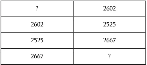
Sliding Window: For a time series problem, in order to apply supervised learning, we need to restructure our data so that it corresponds to a sliding window. Here we use the value at the previous step in order to predict the value at the next step. Therefore the dataset needs to be reorganized in order to predict the correct values.

In sliding window, we reorganized our dataset as shown in the table Fig1 and Fig2. Fig 1 shows the original dataset and Fig2 is the data after modifying it according to the sliding window method

YEARS MURDERS

2001 2602

2002 2525

2003 2667

Figure 1. Murder statistics for three years in Andhra Pradesh

? 2602

2602 2525

2525 2667

2667 ?

Figure 2. The reorganized data according to sliding window method

The first and last rows are removed and we use the rest of the dataset to train the model. In our supervised learning problem, the input(x) will be the

previous time step and the next time step is the output(y). Next we will be able to apply any regression algorithms in order to predict the future values.

We have primarily used three regression algorithms and compared the result to find out which algorithm is giving us the maximum accuracy.

1. Support Vector Regression: It is an extension of the classification theorem Support Vector Machine (SVM). It is used as a regression algorithm with only a few minor differences between the two algorithms. It becomes comparatively difficult to predict a value with the information at hand that can have infinite possibilities. When used as a regression algorithm, a margin of tolerance is set in approximation to the SVM which is a user input at the start of the algorithm itself. SVR has other benefits over SVM, like it minimizes the error in prediction, individualises the hyperplane which maximizes the margin while tolerating a part of the error.

The model produced by SVR depends only on a subset of the training data, because the cost function for building the model ignores any training data that lie close to the prediction model.

2. Decision Tree Regression: A decision tree generates a classification or a regression model in the form of a tree. It divides the dataset into many small subsets, simultaneously incrementally developing a decision tree. The final tree has two different types of nodes, decision nodes and leaf nodes. The decision nodes have two or more child nodes, each representing values for the attribute tested. Leaf nodes represents the target numeric value to be predicted.

(4)

3. Random Forest Regression: It is an ensemble learning method for classification and regression. It operates by constructing multitude of decision trees during training and outputting the class that is the mean prediction of the individual trees. Random Forests are a way of averaging multiple deep decision trees, trained on different parts of the same training dataset, with the goal of reducing the variance. This comes at the expense of a small increase in the bias and loss of interpretability, but greatly boosts the performance in the final model.

IV.

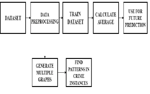
IMPLEMENTATION

The aim of this paper is to find patterns in criminal activities and find the future increase or decrease of a particular criminal activity in the state. This is done so that necessary actions can be taken to curb such activities in that state. In order to achieve the goals, we have used the architecture/workflow diagram as shown in Figure 3.

Figure 3. Workflow Diagram

Multiple dataset files were obtained from government websites which contained the reported number of incidents of each type of crime from 1993 to 2014. After gathering the data, the first step was to preprocess the data. This included two main steps:

first, handling the missing values. The data was

cleaned by removing any inconsistencies and some

missing values were filled in by calculating the mean of the particular attribute and deciding a value around

it. Second, data reduction techniques were applied to

remove any attribute (crime) based on whether it has at least one recorded instance in each state or not. Subsequently, the entire dataset was divided into multiple datasets according to the state and crime using a Python script.

This data was analysed using various time series charts, bar graphs in order to see a pattern in the data. RapidMiner was used for the visualization of the data. The time series graphs was generated using RapidMiner modules and visualization according to various states and crimes. We also generated time series graphs for multiple states and a particular crime in order to get a picture of the scenario of the crime in various states.

After finding patterns in the data, the next step is to predicting future values. This is achieved by training the dataset using various machine learning algorithms. Therefore, we have to convert the dataset into the sliding window format in order to apply supervised learning algorithm as discussed in Section III. This was also achieved using a Python script.

The data was then trained using various machine learning algorithms. The supervised learning algorithms that were applied in the paper were Support Vector Regression, Decision Tree Regression and Random Forest Regression. We divided our data set into the training and testing data. We applied each algorithm separately and trained the training data set. We used Python programming language for each of the algorithm. The scikit_learn library was used for implementing the machine learning algorithms.

(5)

results are from the predicted results. The model which gave the least error was used for the prediction of the crime rates for the future years.

V.

RESULTS AND ANALYSIS

After preprocessing the data multiple time series graphs were generated for various states. The states with the maximum number of murders were obtained as Uttar Pradesh, Maharashtra and Bihar as shown in the Fig4.

Individual time series graphs were also generated for each state and for each crime and the rate of increase/decrease of crime rates in each state could also be analysed. In this way, the government can plan more suitable techniques to handle criminal activities in the area and focus on one or more state or one or more crime than the other.

Figure 4. Time series graph for the states Maharashtra, Uttar Pradesh and Bihar

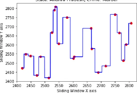
Next the sliding window dataset was trained using the Support Vector Regression, Decision Tree Regression and Random Forest Regression and the training data was plotted as shown in the figures below. The graphs were generated taking into consideration the crime ‘Murder’ for the years 1993-2014 for the state Andhra Pradesh.

Fig5 shows the regression line Decision Tree Regression, Fig6 for Support Vector Regression and Fig7 for Random Forest regression.

Figure 5 Regression Line using Decision Tree Algorithm

(6)

Figure 6. Regression line using Support Vector Regression

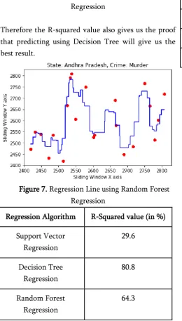
Therefore the R-squared value also gives us the proof that predicting using Decision Tree will give us the best result.

Figure 7. Regression Line using Random Forest Regression

Regression Algorithm R-Squared value (in %)

Support Vector Regression

29.6

Decision Tree Regression

80.8

Random Forest Regression

64.3

Figure 8. R-Squared value for the algorithms

Thus we have calculated the future values of the crimes using the Decision Tree Regression Algorithms. Since we are measuring crime rates and it depends on human psychology, very high R-squared value could not be achieved. The following table in Fig9 shows us the predicted value for some of the crimes in Andhra Pradesh in the year 2018 after applying the Decision Tree algorithm.

CRIME EXPECTED VALUE

2018

Murder 2432

Rape 1070

Dacoity 145

Kidnapping 2119

Figure 9.Expected crime rates in Andhra Pradesh, 2018

VI.

CONCLUSION

The proposed model aims at predicting the total number of incidents of a particular crime in a state. We approached the problem with three different approaches, Support Vector Regression, Decision Tree Regression and Random Forest Regression. The original dataset had to be trained and processed differently for each algorithm. This was accomplished by implementing python scripts.

The data was then fed into the method and a test model was generated. This model was then tested with the help of test values and the model was then made to predict the number of a particular crime that will occur in that state in the given year. The error in the test predictions were very high which led to further training of the models. From the test run of the algorithms it was evident that the Decision Tree Regression algorithm gave the predictions with the best R-squared value.

(7)

use this data to learn how to defend themselves from these threats.

According to our predictions the number of murders in the state of Andhra Pradesh should decrease by 3.68% compared to 2017. The numbers of rape instances are expected to be 1070. Dacoity should decrease down to only 145. A little more effort from everyone and we can bring down this number to 0 in the years to come.

In our analysis high R-squared values could not achieved. This is not due to wrong training of the model but rather because this is a human psychological analysis. There are numerous factors which affect a person’s psychological state, which could lead to committing a crime. The values predicted are based on the past trends in the numbers of crimes committed and does not put a hard value on the numbers predicted.

VII. REFERENCES

[1].Tom M. Mitchell, "Machine Learning"

[2].Vojislav Kecman, "Learning and Soft computing: support vector machines, neural networks and fuzzy logic models"

[3]. https://machinelearningmastery.com/time-series-forecasting-supervised-learning/