University of Windsor University of Windsor
Scholarship at UWindsor
Scholarship at UWindsor
Electronic Theses and Dissertations Theses, Dissertations, and Major Papers
4-30-2018
VIDEO FOREGROUND LOCALIZATION FROM TRADITIONAL
VIDEO FOREGROUND LOCALIZATION FROM TRADITIONAL
METHODS TO DEEP LEARNING
METHODS TO DEEP LEARNING
Thangarajah Akilan University of Windsor
Follow this and additional works at: https://scholar.uwindsor.ca/etd
Recommended Citation Recommended Citation
Akilan, Thangarajah, "VIDEO FOREGROUND LOCALIZATION FROM TRADITIONAL METHODS TO DEEP LEARNING" (2018). Electronic Theses and Dissertations. 7462.
https://scholar.uwindsor.ca/etd/7462
This online database contains the full-text of PhD dissertations and Masters’ theses of University of Windsor students from 1954 forward. These documents are made available for personal study and research purposes only, in accordance with the Canadian Copyright Act and the Creative Commons license—CC BY-NC-ND (Attribution, Non-Commercial, No Derivative Works). Under this license, works must always be attributed to the copyright holder (original author), cannot be used for any commercial purposes, and may not be altered. Any other use would require the permission of the copyright holder. Students may inquire about withdrawing their dissertation and/or thesis from this database. For additional inquiries, please contact the repository administrator via email
VIDEO FOREGROUND LOCALIZATION
FROM TRADITIONAL METHODS TO DEEP LEARNING
by
Thangarajah Akilan
A Dissertation
Submitted to the Faculty of Graduate Studies
through the Department of Electrical and Computer Engineering in Partial Fulfillment of the Requirements for
the Degree of Doctor of Philosophy at the University of Windsor
Windsor, Ontario, Canada
c
VIDEO FOREGROUND LOCALIZATION
FROM TRADITIONAL METHODS TO DEEP LEARNING
by
Thangarajah Akilan
APPROVED BY:
C. Luo, External Examiner University of Detroit Mercy
B. Boufama
School of Computer Science
H. Wu
Electrical and Computer Engineering
M. Khalid
Electrical and Computer Engineering
J. Wu, Advisor
Electrical and Computer Engineering
Declaration of Co-Authorship / Previous
Publication
I Co-Authorship Declaration
I hereby declare that this dissertation incorporates material that is result of joint research, as follows: This dissertation also incorporates the outcome of a research under the supervision of professor Quinmin Jonathan Wu and collaboration with Jie Huo (Chapter 4) and Dr. Yimin Yang (Chapter 6). The research under Prof. QMJ Wu is covered in Chapter 4, 5, 6, 7, 8, and 9 of the dissertation. In all cases, the key ideas, primary contributions, experimental designs, data analysis, interpretation, and writing were performed by the author, and the contribution of the coauthors was primarily through the provision of proof reading and reviewing the research papers regarding the technical content.
I am aware of the University of Windsor Senate Policy on Authorship and I certify that I have properly acknowledged the contribution of other researchers to my disser-tation, and have obtained written permission from each of the co-authors to include the above materials in my dissertation.
I certify that, with the above qualification, this dissertation, and the research to which it refers, is the product of my own work.
II Previous Publication
This dissertation includes seven original papers that have been previously published/un-der review in peer reviewed journals and conferences, as follows:
Thesis
Chapter Publication title/full citation
Publication status
Chapter 4
T. Akilan, QMJ. Wu, ”Video foreground detection in non-static background using multi-dimensional color space.” Procedia Computer Science 70 (2015): 55-61,
c
2015 Elsevier.
Published
Chapter 5
T. Akilan, QMJ. Wu, and J. Huo. ”A unified thresh-old updating strategy for multivariate Gaussian mix-ture based moving object detection.” High Performance Computing & Simulation (HPCS), 2016 International Conference on. IEEE, c2016 IEEE.
Chapter 6
T. Akilan, QMJ. Wu, and Y. Yang. ”Fusion-based fore-ground enhancement for backfore-ground subtraction using multivariate multi-model Gaussian distribution.” Infor-mation Sciences 430 (2018): 414-431, c2017 Elsevier.
Published
Chapter 7
T. Akilan, and QMJ. Wu, ”sEnDec: An improved im-age to imim-age CNN for foreground localization,” IEEE Intelligent Transportation Systems Transactions.
Under review
T. Akilan, and QMJ. Wu, ”Double Encoding - Slow De-coding Image to Image CNN for Foreground Identifica-tion with ApplicaIdentifica-tion Towards Intelligent Transporta-tion,” IEEE GreenCom 2018.
Submitted
Chapter 8
T. Akilan, and QMJ. Wu, ”An Improved Video-foreground Extraction Strategy Using Multi-view Re-ceptive Field and EnDec CNN,” IEEE Transactions on Industrial Informatics.
Under review
Chapter 9
T. Akilan, and QMJ. Wu, et al. ”A 3D CNN-LSTM based image-to-image foreground segmentation,” IEEE Intelligent Transportation Systems Transactions.
Under review
I certify that I have obtained a written permission from the copyright owners to include the above published materials in my dissertation. I certify that the above material describes work completed during my registration as graduate student at the University of Windsor.
III General
Abstract
These days, detection of Visual Attention Regions (VAR), such as moving ob-jects has become an integral part of many Computer Vision applications, viz. pat-tern recognition, object detection and classification, video surveillance, autonomous driving, human-machine interaction (HMI), and so forth. The moving object iden-tification using bounding boxes has matured to the level of localizing the objects along their rigid borders and the process is called foreground localization (FGL). Over the decades, many image segmentation methodologies have been well studied, devised, and extended to suit the video FGL. Despite that, still, the problem of video foreground (FG) segmentation remains an intriguing task yet appealing due to its ill-posed nature and myriad of applications. Maintaining spatial and temporal co-herence, particularly at object boundaries, persists challenging, and computationally burdensome. It even gets harder when the background possesses dynamic nature, like swaying tree branches or shimmering water body, and illumination variations, shadows cast by the moving objects, or when the video sequences have jittery frames caused by vibrating or unstable camera mounts on a surveillance post or moving robot. At the same time, in the analysis of traffic flow or human activity, the perfor-mance of an intelligent system substantially depends on its robustness of localizing the VAR, i.e., the FG. To this end, the natural question arises as what is the best way to deal with these challenges?
This thesis is dedicated to
my late mother, Vijayaluxmi.
I miss her every moment, but
I feel that she saw this process through to its completion,
Acknowledgements
Foremost, I would like to express my sincere gratitude to my advisor, Dr. Q.M. Jonathan Wu for giving me the opportunity to work under his supervision as well as for his guidance and continuous support for my Ph.D study and research. I also thank my committee members Dr. M. Khalid, Dr. H. Wu, and Dr. B. Boufama for guiding me and helping me with their invaluable comments. I heartily thank our department graduate secretary Ms. Andria Ballo, who has helped me in so many situations that I cannot possibly list in this limited space. Finally, I would like to convey my earnest gratitude to the Golden Key International Honour Society for bestowing me with the prestigious Golden Keys premier scholarship.
The person, who guided me to resume studies after nearly a decade of a debacle life, continuously provided support, is my cousin Dr. Esai Selvarasa. I would like to convey my sincere thanks to her. I could not have come this far without the help from my fellow lab members, and would like to thank them for supporting me. A special thank goes to the department technician Mr. Frank Cicchello, who helped me whenever I requested, even during his most busy hours.
I like to convey my regards, and sincere gratitude to my parents, my brother, sisters, cousins, and my in-laws. Under inexpressible circumstances and financial difficulties, they stand with me as strong pillars of support. I cannot thank them enough for their sacrifices and patience. I convey my gratitude to my father and late-mother for their continuous support and unfathomable trust. I would like to extend my sincere appreciation to Dr. Mohd Amaludin Yusoff for his motivational advice whenever I fell in the midst of confusion. His guidance helped me in all the time of research and life.
Table of contents
Declaration of Co-Authorship / Previous Publication iii
Abstract v
Dedication vii
Acknowledgements viii
List of tables xiv
List of figures xvi
List of abbreviation xxii
1 Introduction 1
1.1 Overview . . . 1
1.2 Motivation . . . 1
1.3 Evaluation of foreground localization . . . 4
1.4 Contributions to knowledge . . . 5
1.5 Methodology . . . 6
1.6 Research findings . . . 7
1.7 Thesis structure . . . 8
2 Background 10 2.1 Overview . . . 10
2.2 Computer vision . . . 10
2.3 Foreground . . . 10
2.4 Background . . . 10
2.5 Foreground localization . . . 11
2.6 Background subtraction . . . 11
2.7 Gaussian mixture models . . . 11
2.7.2 Multivariate distribution . . . 12
2.7.2.1 The covariance matrix . . . 13
2.7.2.2 Generalization . . . 14
2.8 Deep learning . . . 15
2.9 Convolutional neural network . . . 15
2.9.1 Convolution layers . . . 17
2.9.2 Densely connected layers . . . 17
2.10 Activation function . . . 18
2.10.1 ReLU . . . 19
2.10.2 Sigmoid . . . 19
2.10.3 Softmax . . . 20
2.10.4 Batch normalization . . . 20
2.11 Long-short term memory . . . 21
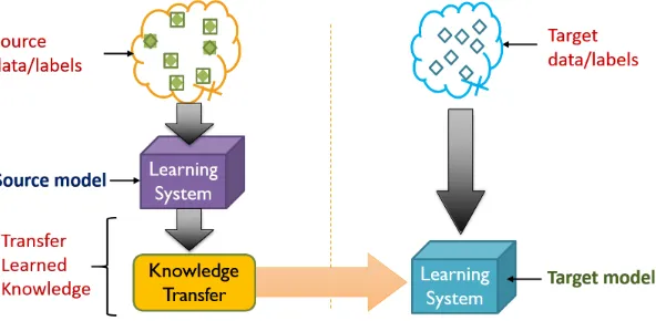
2.12 Transfer learning . . . 22
3 Literate review 24 3.1 Pixel-based background modeling . . . 26
3.2 Region-based background modeling . . . 28
3.3 Hybrid background modeling . . . 31
3.4 CNN-based semantic segmentation to FGL . . . 32
4 Video foreground detection in non-static background using multi-dimensional color space 37 4.1 Summary . . . 37
4.2 Introduction . . . 37
4.3 The algorithm . . . 38
4.3.1 Probabilistic-based background suppression with non-supervised threshold 38 4.3.2 Euclidean distance-based background suppression in 3D-color space . . 40
4.4 Experimental results . . . 42
4.5 Discussion and conclusion . . . 44
5 A Unified Threshold Updating Strategy for Multivariate Gaussian Mixture Based Moving Object Detection 46 5.1 Summary . . . 46
5.2 Introduction . . . 46
5.3 Proposed Algorithm . . . 48
5.3.2 Threshold updating . . . 51
5.3.3 Foreground refinement . . . 52
5.4 Experimental results . . . 53
5.4.1 Nature of the experiments . . . 53
5.4.2 Visual results . . . 54
5.4.3 Quantitative analysis . . . 54
5.5 Conclusion . . . 56
6 Fusion-based Foreground Enhancement for Background Subtraction Using Multivariate Multi-model Gaussian Distribution 57 6.1 Summary . . . 57
6.2 Introduction . . . 58
6.3 The proposed algorithm . . . 59
6.3.1 The applied multivariate Gaussian mixture model . . . 59
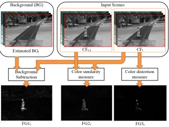
6.3.2 The proposed framework . . . 60
6.3.2.1 Background estimation . . . 61
6.3.3 Color similarity measure . . . 63
6.3.4 Color distortion measure . . . 64
6.3.5 FG feature enhancement and detection . . . 65
6.3.6 Foreground validation . . . 68
6.4 Experimental results . . . 70
6.4.1 Qualitative analysis . . . 71
6.4.2 Quantitative analysis . . . 74
6.4.3 Contribution of the features . . . 76
6.4.4 Fully utilized MVGMD . . . 77
6.4.5 Limitations of the proposed model . . . 78
6.5 Conclusion . . . 80
7 sEnDec: An Improved Image to Image CNN for Foreground Local-ization 81 7.1 Summary . . . 81
7.2 Introduction . . . 82
7.3 The proposed CNN architecture: sEnDec . . . 84
7.3.1 Deep slow encoding . . . 86
7.3.2 Deep slow decoding . . . 86
7.3.3 Training strategy . . . 87
7.3.5 Environment . . . 90
7.4 Experimental setup, results, and discussion . . . 90
7.4.1 Dataset . . . 90
7.4.1.1 Training and test sets . . . 91
7.4.2 Evaluation . . . 92
7.4.3 Step-by-step analysis . . . 92
7.4.3.1 Sanity check . . . 92
7.4.3.2 Visual analysis . . . 93
7.4.3.3 Numerical analysis . . . 96
7.4.4 Extended experiment . . . 98
7.4.4.1 Subjective analysis . . . 99
7.4.4.2 Objective analysis . . . 99
7.5 Conclusion . . . 104
8 An Improved Video-foreground Extraction Strategy Using Multi-view Receptive Field and EnDec CNN 105 8.1 Summary . . . 105
8.2 Introduction . . . 106
8.3 Proposed MV-FCN architecture . . . 109
8.3.1 Training strategy . . . 112
8.3.1.1 Exclusive sets . . . 112
8.3.1.2 Input configuration . . . 112
8.3.1.3 Optimizer . . . 113
8.3.1.4 Transfer learning . . . 113
8.3.1.5 Training environment: . . . 114
8.3.2 Binary foreground mask . . . 114
8.4 Experimental setup, results, and discussion . . . 115
8.4.1 Step-by-step analysis . . . 116
8.4.1.1 Impact of complimentary feature flows . . . 116
8.4.1.2 Impact of transfer learning . . . 118
8.4.1.3 Qualitative analysis . . . 120
8.4.1.4 Quantitative analysis . . . 121
9 A 3D CNN-LSTM Based Image-to-Image Foreground Segmentation128
9.1 Summary . . . 128
9.2 Introduction . . . 129
9.3 The CNN-LSTM based foreground segmenter . . . 131
9.3.1 ConvLSTM layers . . . 134
9.3.2 Transpose convolution . . . 136
9.3.3 Activation functions . . . 136
9.3.4 Training strategy . . . 137
9.3.5 Binary foreground mask . . . 139
9.4 Experimental setup, results, and discussion . . . 140
9.4.1 Qualitative analysis . . . 141
9.4.2 Quantitative analysis . . . 143
9.5 Conclusion . . . 145
10 Conclusion 147 10.1 Contributions and limitations . . . 147
10.1.1 Traditional methods . . . 148
10.1.2 Deep learning-based models . . . 150
10.2 Applications . . . 152
10.3 Dissemination . . . 152
Bibliography 153
A IEEE Permission to Reprint 172
B Elsevier Permission to Reprint 173
C Code Samples 174
List of tables
1.1 Confusion matrix. . . 4
4.1 Performance comparison of the proposed algorithms for WaterSurface dataset. 43 4.2 Performance comparison of the proposed algorithms for WavingTree dataset. 43 5.1 Description of the datasets used for validation. . . 53
5.2 Performance comparison. The best figures are in red ink. . . 55
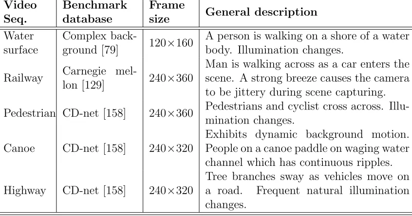
6.1 Description of the video sequences used for validation. . . 70
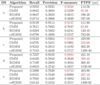
6.2 Average F-measure Comparison on Railway data sequence . . . 75
6.3 Average F-Measure Comparison On Watersurface Data Sequence . . . . 75
6.4 Average F-Measure Comparison On Pedestrian, Highway, And Canoe Data Sequences . . . 75
6.5 Average PTPF (in Sec.) Comparison On Pedestrian, Highway, And Canoe Data Sequences . . . 76
6.6 Impact of fully utilized MVGMD in terms of FoM . . . 78
7.1 The dataset pairs involved in model initialization. . . 88
7.2 The environment. . . 90
7.3 Dataset summary. . . 91
7.4 Sanity check results of the proposed sEnDec compared to the basic model. 93 7.5 F-measure-based performance comparison: G-th, O-th, and OG-th stand for global, Otsu, and Gaussian smoothed Otsu threshold methods ap-plied, respectively. The values in red and blue are the best and the second best figures, respectively. . . 97
7.6 F-measure performance comparison: G-th, O-th, KI-th, and BGM stand for binarization methods with global, Otsu and Kittler-Illingworth thresholdings, and variational Bayesian Gaussian distribution, respec-tively. The values in red and blue are the best and the second best figures, respectively. . . 103
8.2 Dataset summary. . . 111
8.3 Transfer learning detail for fine-tuning the proposed MV-FCN. . . 113
8.4 Results: impact of complimentary feature flows. . . 116
8.5 Performance comparison of random vs transfer learning-based model ini-tialization in terms of f-measure: S and P stand for type of training strategy, scratch and fine tuning pre-trained model. Global and Otsu threshold methods are referred by G-th and O-th respectively. . . 118
8.6 F-measure performance comparison: S- training from scratch, P- pre-trained model fine-tuning, Global and Otsu stand for the two used thresholding methods. Values in red are the best figures while the ones in blue are the second best. . . 124
9.1 Layer detail of the proposed 3D CNN-LSTM. . . 134
9.2 Dataset summary. . . 137
9.3 The dataset pairs used for model fine-tuning. . . 139
9.4 Performance Comparison in terms of FoM: Global-th and Otsu-th stand for the two thresholding methods applied. Values in red are the best FoM while the ones in blue are the second best. . . 144
List of figures
1.1 Examples for video surveillance camera placements. . . 2
1.2 Applications of video cameras: (a) AImotive’s customized Toyota Prius has cameras in front, on its sides, and in back. (b) Onboard cameras are key to developing truly independent robots. . . 2
1.3 A probable application environment of foreground localization. . . 3
2.1 A background subtraction paradigm. . . 11
2.2 Plots of a bivariate normal distribution. . . 13
2.3 A Vann diagram showing how deep learning (DL) is a kind of representa-tion learning, which is in turn a part of machine learning (ML). . . . 15
2.4 Deep learning to convolutional neural network. . . 16
2.5 An example of CNN architecture: A handwritten digit classifier. . . 16
2.6 Convolution feature map generation in LeNet5 [77]. . . 18
2.7 An example of top fully connected layer. . . 18
2.8 Block diagram describing transfer learning technique. . . 22
3.1 A scene and its useful region of interest. . . 24
3.2 Categories of foreground localization algorithms. . . 25
3.3 CNN feature flows: (a) ResNet flow, and (b) the residual feature mapping of our models. . . 33
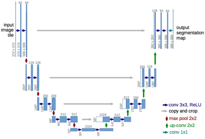
3.4 U-net architecture. Blue boxes correspond to a multi-channel feature map. The number of channels is denoted on top of the boxes. The x-y-size is provided at the lower left edge of the box. White boxes represent copied feature maps and the arrows refer to the different type of operations [119]. 34 3.5 The network is trained with two small patches extracted from the in-put and background images in gray-scale. The network is inspired by LeNet-5 network [17]. . . 36
4.2 3D Geometrical representation of (a). PointP, (b). PointP0, and (c) The
distance between P and P0. . . . 40
4.3 Example of 3D-color space. . . 41
4.4 Sample results for the WaterSurface dataset. . . 43
4.5 Sample results for the WavingTree dataset. . . 43
4.6 Average performance comparison across all the color-spaces and datasets. 44 5.1 Process-flow of the proposed algorithm. . . 48
5.2 Unclassified FG Region. . . 51
5.3 Visual comparisons of the results for frames no. 250 - 1st row and no. 559 - 2nd row form datasets (a) and (b), respectively. . . 54
5.4 Visual comparisons of the results for frames 435 - 1st row, 626 - 2nd row, and 827 3rd row from datasets (c) - (e) respectively. . . 54
5.5 Performance comparison. . . 55
6.1 A scene and its useful region of interest. . . 58
6.2 First level of foreground features. . . 61
6.3 Fused foreground features and its corresponding intensity histogram. . . 61
6.4 Step diagram of color similarity calculation through CIEDE2000. . . 64
6.5 Optimal threshold adjustment in the histogram of enhanced FG features. 66 6.6 Detected FG with optimal threshold. . . 68
6.7 Validated foreground. . . 68
6.8 Process block diagram of the proposed algorithm. . . 68
6.9 Comparisons of foreground extraction for Railway data sequence: (a). original scene, (b). ground truth, and (c) to (i) show the detected FG of different methods GMM, EGMM, BOD, S-SVM, DECOLOR, Ours, and OursKIth respectively. . . . 72
6.10 Comparisons of FG separation for WaterSurface data sequence: (a). orig-inal scene, (b). ground truth, and (c) to (i) show the detected FG of different methods GMM, EGMM, FCH, RPCA, DECOLOR, Ours, and OursKIth respectively. . . . 72
6.12 Comparisons of FG separation on Highway data sequence: Columns (a) to (h) show original significant scenes with frame IDs embedded, ground truth, and extracted FG of different methods CRF, EGMM, GMM,
waVGMM, Ours, and OursKIth respectively. . . . 74
6.13 Comparisons of FG separation Canoe data sequence: Columns (a) to (h) show original significant scenes with frame IDs embedded, ground truth, and detected FG of different methods CRF, EGMM, GMM, waVGMM, Ours, and OursKIth respectively. . . . 74
6.14 F-Measure comparison on various input feeds vs methods. . . 76
6.15 Processing time comparison on various input feeds vs methods. . . 77
6.16 Processing time of the proposed algorithm vs input feeds. . . 77
6.17 FoM error bar vs level of fused FG features. . . 78
6.18 BusStation frame no. 1096: The proposed model fails to distinguish mov-ing shadow and sudden region level changes. . . 79
6.19 Bungalows frame no. 650: The proposed model fails to distinguish the moving shadow. . . 79
7.1 Block diagram of a basic image-to-image CNN. . . 82
7.2 Schematic drawing of the proposed DCNN: sEnDec. . . 84
7.3 Illustration of convolution and transpose (de) convolution operations: A 2D conv with K = 3, S = 2, and P = 1, and its corresponding convT with K0 =K, S0 = 1, and P0 =K−P −1. . . . 85
7.4 The exploited residual feature flow and resolution recovery mechanism. . 87
7.5 Input data configuration:G.T-Ground truth, I-Image, M ed(·)- Median fil-tering in temporal domain over collected k samples prior to training, b0 - The precomputed BG model, and ft - Input scene at time t. . . . 88
7.6 Random vs ordered splits: G.T- ground truth, I- raw image, Sq.#- se-quence ID. . . 92
7.7 Bar chart comparison- sanity test results of the sEnDec and basic model: F-measure vs video sequences. . . 93
7.9 Sample results. Row 1-8: Traffic, Boulevard, CopyMachine, PeopleIn-Shade, BusStation, Sofa, Tramstop, and SnowFall video sequences. Col. 1-5: input frames, ground truths, sEnDec’s score-maps, binary FG masks generated with G-th and O-th, respectively. . . 95 7.10 Sequence category-wise performance analysis. . . 96 7.11 Overall performance analysis of various models. . . 98 7.12 F-measure vs model: Performance analysis across all the video sequences. 99 7.13 F-measure vs binarization method. . . 100 7.14 Processing time vs binarization method. . . 100 7.15 FGL speed of sEnDec including binary mask creation. . . 101 7.16 Subjective analysis on the CD-net [158] benchmark database. Sample
re-sults - Row 1-10: Highway, Office, Pedestrians, PETS2006, Fall, Traf-fic, Boulevard, BusStation, Sofa, and Tramstop video sequences. . . . 102
8.1 The ResNet-like and Inception-like modules. . . 108 8.2 Layer schematic of the MV-FCN: Convk, Si, CTransk, Concat, and BN
stand for convolution using kernel size of k and stride of i, transpose convolution with filter size of k, activation maps concatenation, and batch normalization operations, respectively. . . 109 8.3 Ordered exclusive split of training and test sets: G.T- ground truth,
I-RGB raw input image, S.q#- sequence ID. . . 112 8.4 Creating FG mask: Applying an appropriate threshold to the score-map
generated from the last classification layer of MV-FCN for a frame taken from the Office dataset. . . 114 8.5 Network configurations for investigating impact of complimentary feature
flows. . . 117 8.6 Visualizing impact of complimentary feature flows: (a) Input frame, (b)
-(e) are the salient map of PFF, combined feature flow of PFF & CFF2, PFF & CFF1, and PFF & CFF1 & CFF2, respectively. . . 118 8.7 Performance vs model initialization in terms of f-measure: S and P stand
for type of training strategy, scratch and fine tuning pre-trained model. Global and Otsu threshold methods are referred by G-th and O-th respectively. . . 119 8.8 MV-FCN salient map when: (b) trained from scratch, (c) fine-tuned with
8.9 Office dataset. Col. 1-5: Sample input frames, MV-FCN generated score-maps, binary FG masks with empirical and Otsu’s thresholds. Col. 6: training and validation FoM and loss respectively in the top and bottom.120 8.10 Overpass dataset. Col. 1-5: Sample input frames, MV-FCN generated
score-maps, binary FG masks with empirical and Otsu’s thresholds. Col. 6: Training and validation FoM and loss respectively in the top
and bottom. . . 121
8.11 Traffic dataset. Col. 1-5: Sample input frames, MV-FCN generated score-maps, binary FG masks with empirical and Otsu’s thresholds. Col. 6: Training and validation FoM and loss respectively in the top and bottom.121 8.12 PeopleInShade dataset. Col. 1-5: Sample input frames, MV-FCN gener-ated score-maps, binary FG masks with empirical and Otsu’s thresh-olds. Col. 6: Training and validation FoM and loss respectively in the top and bottom. . . 122
8.13 TwoPositionPTZCam dataset. Col. 1-5: Sample input frames, MV-FCN generated score-maps, binary FG masks with empirical and Otsu’s thresholds. Col. 6: Training and validation FoM and loss respectively in the top and bottom. . . 122
8.14 Turnpike 0 5fps dataset. Col. 1-5: Sample input frames, MV-FCN gener-ated score-maps, binary FG masks with empirical and Otsu’s thresh-olds. Col. 6: Training and validation FoM and loss respectively in the top and bottom. . . 123
8.15 Performance comparison: F-measure vs method. . . 125
8.16 Best performance comparison: F-measure vs dataset. . . 125
8.17 Inferencing speed of the proposed MV-FCN. . . 126
9.1 Traffic flow and its foreground (Input frame, Ground truth, 3D CNN-LSTM score-map, and Predicted FG mask). . . 129
9.2 An overview of the proposed CNN-LSTM image-to-image network: E(·) -binary cross-entropy error. . . 130
9.3 A layer-wise schematic of the proposed 3D CNN-LSTM. It exploits 3D conv embedded with 2D LSTM both in the encoding and decoding phases, and residual layer concatenation and 3D transpose conv layers only in the decoding subnetwork. . . 132
9.4 Simplified 3D CNN-LSTM model with single stage EnDec. . . 133
List of abbreviation
1D One-Dimension or One-Dimensional
2D Two-Dimension or Two-Dimensional
3D Three-Dimension or Three-Dimensional
AI Artificial Intelligence
BN Batch Normalization
BG Background
BGS Background Subtraction
BOD Bayesian Object detection in Dynamic scenes
BRDL Background subtraction via Robust Dictionary Learning
CEC Constant Error Carousel
CFF Complementary Feature Flows
CNN or ConvNet Convolutional Neural Network
CPU Central Processing Unit
CRF Conditional Random Field
CTC Connectionist Temporal Classification
CTrans Transpose Convolutional
CV Computer Vision
DBFCN Deep Background Fully Convolutional Network
DCNN Deep Convolutional Neural Network
DConv Deconvolution
CD Change Detection
DESD Double Encoding Slow Decoding
DL Deep Learning
DPMM Dirichlet Process Mixture Models
EnDec Encoder-Decoder
FCH Fuzzy Color Histogram
FCN Fully Convolutional Network
FG Foreground
FGL Foreground Localization
FN False Negative
FOV Field of View
FP False Positive
FPS Frame Per Second
GMM Gaussian Mixture Model
GP Genetic Programming
GPU Graphic Processing Unit
GT Ground Truth
GTI Generalized Tverksy Index
HMI Human Machine Interaction
HPC High Performance Computing
ILSVRC Large-Scale Visual Recognition Challenge
IoU Intersection Over Union
KDE Kernel Density Estimation
LBP Local Binary Pattern
LBSP Local Binary Similarity Pattern
LRE Local Refinement Error
LSTM Long-Short Term Memory
LTP Local Ternary Pattern
MCR Missed-classification Ratio
MKFC Multi-channel kernel fuzzy Correlogram
MP Mega-Pixel
MRF Markov Random Field
MRI Magnetic Resonance Imaging
MVGMM Multivariate GMM
MVGMD Multivariate Gaussian Model Distribution
MV-FCN Multi-View receptive field FCN
NN Neural Networks
ORDL Online Robust Dictionary Learning
OR-PCA Robust Online PCA
OS Operating System
PBAS Pixel-Based Adaptive Segmenter
PCA Principal Component Analysis
PFF Pivotal Feature Flow
PRI Probabilistic Rand Index
RAM Random Access Memory
RGB Red Green Blue
ReLU Rectified Linear Unit
ResNet Residual Network
RNN Recurrent Neural Network
RRC Radial reach correlation
RPCA robust principal component analysis
ROI Region of Interest
SACON SAmple CONsensus
SDAE Stacked Denoising Auto-Encoder
sEnDec Slow Encoder-Decoder
SOM Self-Organizing Map
SuBSENSE Self-Balanced SENsitivity SEgmenter
SVD Singular Value Decomposition
TL Transfer Learning
TN True Negative
TP True Positive
VAR Visual Attention Region
VCA Video Content Analysis
VCAP Video Content Aware Processing
VCAA Video Content Aware Applications
ViBe Visual Background extractor
Chapter 1
Introduction
1.1
Overview
This chapter elaborates the motivation, aims, and objectives of the research, and provides the background information of foreground localization. Furthermore, the key contributions and methodology are briefly disclosed. Finally, the thesis structure is outlined.
1.2
Motivation
capable of automatically extracting application-specific information, for instance, the presence of an object, in the scene being monitored. The system can be a tool to help humans to perform intriguing and time-consuming tasks and to maintain the efficiency of video-based applications by processing only relevant detail. Most video data have redundant information, such as background information, which costs a massive volume of storage and computing resources.
Moreover, the scenes monitored exhibit illumination changes, motion changes, secondary illumination effects cast by the moving objects, and random pixel intensity variations due to capturing devices. To this end, what is the best way to deal with these challenges? At the same time, in the analysis of traffic flow or human activity, the performance of an intelligent system substantially depends on its robustness of foreground localization [170].
The goal of this thesis is to improve the fundamental algorithms and introduce new deep learning architectures for foreground localization that can be applicable to many Video Content Aware Applications (VCAA).
(Image: https://ihsmarkit.com,https://www.envisioninteligence.com)
Figure 1.1: Examples for video surveillance camera placements.
(a) (b)
(Image: http://www.businessinsider.com,https://cosmosmagazine.com)
The applications of FGL is myriad as a probable application environment depicted by Fig. 1.3. For example, the FGL-based automatic people and vehicle detection, counting, and tracking system can address the following sectors:
Figure 1.3: A probable application environment of foreground localization.
• Object recognition: In general, recognition identifies an object to be part of a group of objects. This process can be carried out by object segmentation and extraction followed by a classification task. For instance, in case of traffic signal recognition, where the traffic signal is segmented into a single object based on some primitive features, such as color intensities and texture information; later, it is recognized to identify the class of traffic signals. Thus, such systems require FG segmentation mechanism to locate the specific object in a video frame or image.
• Security: Many industries or public facilities such as airports are interested in locating and tracking people to monitor human presence in forbidden areas, like borders crossings, or people walking in wrong directions, and suspicious activities can be automatically detected and shared with security agents.
• Human gesture or action recognition: It is a rapidly growing application area of foreground detection/localization. The FG identification is employed at an early stage to extract the human or simply the gesture to process towards the recognition or classification stage [124, 125].
• Data compression: Content-aware data compression that keeps intact the essential foreground objects while applying higher data compression rate on the background for big video data.
• Optimization: Based on the detected FG, a system can perform object index-ing for statistical analysis on the people on a platform, for instance, to optimize flows in railways. It can help to answer - How many people are waiting? How long? Moreover, where are they usually going? Thus, peak times can be iden-tified to optimize operation.
• Autonomous driving and traffic safety: It assists in getting accurate vi-sual perception around a vehicle resulting in improved road traffic safety and autonomous navigation.
1.3
Evaluation of foreground localization
Predicted Class Positive Negative
Actual Class Positive TP FN
Negative FP TN
Table 1.1: Confusion matrix.
There are many objective evaluations methods, like Local Refinement Error (LRE), Missed-classification Ratio (MCR), Probabilistic Rand Index (PRI), Variation of In-formation (VoI), and F-measure. Among them, the f-measure is the most widely accepted and standardized method, which is a weighted harmonic mean measure of recall and precision, i.e., size of the intersection divided by the union of the two regions. It is also referred as Intersection-over-Union (IoU) or Figure-of-Merit (FoM) and defined as (1.1).
F −measure= 2×(P recision×Recall)
P recision+Recall , (1.1)
where recall is the detection rate and precision is the percentage of correct prediction compared to the total number of detections as positives. The recall and precision are given by (1.2), where T P, F N, and F P refer true positive, false negative, and false positive, respectively as described by the confusion matrix in Table 1.1.
Recall= T P
T P +F N, P recision=
T P
T P +F P (1.2)
1.4
Contributions to knowledge
A reliable FG localization algorithm should be robust and able to handle sudden and gradual illumination changes, high frequency moving objects, repetitive motion in the background (such as tree leaves, flags, waves in the sea or lake, etc.) and long-term scene changes (a car is parked for a month, for instance). Thus, there have been many algorithms proposed fundamentally based on GMM by the CV com-munity over the past two decades since the pioneer work reported by Stauffer and Grimson [139]. For instance, Effective GMM [78], GMM-based conditional random filed [159, 160], Variational clustered GMM [24], and Wavelet transformation-based GMM [91]. However, such high complexity algorithms are not necessary for specific surveillance purposes, including monitoring an automatic teller machine (ATM) in a shopping complex or bank. Because in such cases, the surveillance camera is fixed at a place and the background environment is known prior to monitoring. In such con-ditions, it is recommended to employ simplistic models to the moving objects in the given environment being monitored. To this end, this thesis, firstly, introduces two simplistic algorithms: a probabilistic based model with a non-supervised threshold and 3D-color space model using distance vector for constrained environment BGS. The outcomes of these models have been published in [144].
major processing stages: BG estimation and FG detection, FG feature enhancement, and FG refinement. The outcomes of the improved model have been published in [3]. It is also very crucial to adopt the cutting-edge CV technologies, like DL for FGL. Deep learning networks have been successfully applied to big data for knowledge discovery, knowledge application, and knowledge-based prediction. Consequently, the deep CNN has become a driving force of the modern era autonomous driving, video surveillance, drug and food inspection, and so forth. Thus, this thesis also extends the work on utilizing DL for FG. It harnesses the power of CNN-based image semantic segmentation ideas for video foreground localization. It improves the basic EnDec CNN through the following innovative approaches:
1. Slow encoder-decoder CNN with micro auto-encoder blocks, batch normaliza-tion, and channel-wise residual feature concatenation.
2. Multi-view receptive field to capture scale-invariant features of FG objects.
3. CNN-LSTM model to exploit spatiotemporal cues for delineate FGL.
Finally, this thesis analyses the performances of the proposed approaches on pub-licly available benchmark data-sets for video FGL. All the findings at every stage of the research have been published through or submitted to internationally recognized IEEE conferences, journals, and transactions.
1.5
Methodology
The following research methodology is pursued for this doctorate:
• Literature review: An extensive background study was conducted on the exist-ing works in the area of foreground localization. Research articles and papers published by official international conferences and journals were reviewed in depth to understand the research carried out so far in the field of FGL to find research gaps and to set the milestones of this thesis. The papers studied are mainly from IEEE, ACM, IET, Elsevier, and Springer.
the classical image processing book, Digital Image Processing by G. Woods [43] to online resources, the Stanford CS231n - Convolutional Neural Networks for Visual Recognition [38].
• Programming paradigm: Python with Keras using Tensorflow backend and MATLAB were used to develop algorithms and DL models for FGL and to test and verify the output of the proposed logic(s).
• Data-sets: In order to test the algorithms and models, publicly available bench-mark video sequences with varying challenges are used. Moreover, the results achieved are analyzed with ground-truths and quantitatively compared to liter-ature results using standard measurement matrices. The performance measures indicate the strength and weakness of the proposed algorithms and models over the existing works by other researchers.
• Dissemination: The outcomes are presented at and/or disseminated through IEEE international conferences, transactions, and international journals, like IET, and Springer whereby the proposed work are reviewed by experts in the field. Experts’ feedback is one of the rich sources towards the advancement of knowledge that is used for continuous improvement of the proposed methods.
• Knowledge exchange: We conduct regular seminars with our peers at our com-puter vision and sensing systems laboratory (CVSSL) and meet experts at var-ious conferences as another source of gaining knowledge.
1.6
Research findings
During this doctorate research the proposed methodologies and related works have been published and/or presented in international IEEE conferences, journals, and transactions. The list of publications as follows:
• T Akilan, QMJ Wu, Y Yang, Fusion-based foreground enhancement for back-ground subtraction using multivariate multi-model Gaussian distribution, Jour-nal of Information Sciences, 430, 414-431, 2018 (IF >4.5).
• T Akilan, QMJ Wu, et al., A 3D CNN-LSTM-based image-to-image foreground segmentation, IEEE Trans. ITS, 2018 (Under review: T-ITS-18-01-0043).
• T. Akilan, and QMJ Wu, Double encoding - Slow decoding image to image CNN for foreground identification with application towards intelligent transportation, IEEE GreenCom 2018 (Submitted: #1570441560).
• T Akilan, and QMJ Wu, An improved video-foreground extraction strategy using multi-view receptive field and EnDec CNN, IEEE Trans. on Broadcasting, 2018 (Under review: BTS-18-058).
• T Akilan, QMJ Wu, et al., Effect of fusing features from multiple dcnn archi-tectures in image classification, IET Image Process., 2018.
• T Akilan, QMJ Wu, et al., A late fusion approach for harnessing multi-cnn model high-level features, IEEE Int. Conf. SMC, 2017.
• T Akilan, QMJ Wu, et al., A feature embedding strategy for high-level cnn representations from multiple convnets, IEEE GCSSIP, 2017.
• T Akilan, QMJ Wu, et al., Fusion of transfer learning features and its applica-tion in image classificaapplica-tion, IEEE CCECE, 2017.
• T Akilan, QMJ Wu, and J Huo, A unified threshold updating strategy for multivariate gaussian mixture based moving object detection, Intr. Conf. High Performance Computing & Simulation (HPCS), 570-574. IEEE, 2016.
• T Akilan, QMJ Wu, et al., Video foreground detection in non-static back-ground using multi-dimensional color space, Procedia Computer Science 70, 55-61, 2015.
1.7
Thesis structure
This thesis consists of ten chapters, initially with this introductory chapters, which provide a concise synopsis of the work. Gradually, it spans out on proposed algo-rithms and models. Finally, it concludes with discussions and directions for future work. It is structured as follows:
contributions in the field. However, in the core chapters also the relevant literature reviews are given in concise form whenever it is possible to enhance the understanding of the proposed ideas.
Chapter 4 proposes two sample-based FGL algorithms using probability mass func-tion with a non-supervised threshold computafunc-tion and a 3D-color space model using distance vector for background suppression. Empirical study is carried out with var-ious color spaces, like RGB, YCbCr, YIQ, and YUV.
Chapters 5 and 6 intent to present novel ideas to update the threshold of GMM-based BGS with respect to color distortion, similarity and illumination measures in pixel-level. These cues are interesting as the CIDE2000 color similarity and color distortion have not been used for foreground localization by the CV community so far.
Chapter 7 introduces two elegant ideas to improve the learning ability of a basic image-to-image CNN network through micro-auto-encoder blocks in the subsampling subnetwork and slow decoding blocks in the upsampling subnetwork.
Chapter 8 introduces akin to Inception modules with multi-view receptive field to capture scale invariant FG clues. And to capture the spatiotemporal features, it uses a temporally median filtered BG model stacked as the third channel of input data that takes two consecutive frames as the first two channels.
Chapter 9 harnesses the ability of LSTM modules in handling time series data. It implements a 3D CNN-LSTM network that takes four frames at a time to predict the FG region in the current frame.
Chapter 2
Background
2.1
Overview
This chapter lays a strong foundation of the dissertation by providing the definitions, mathematical derivations, and background information on the key topics relevant to the work presented.
2.2
Computer vision
Computer vision is the science that focuses on the ultimate goal of creating a similar, if not better, the capability of the human vision system (the way eyes and brain work together) to a machine or computer. The core components of CV are: an automatic feature extraction, analysis and understanding of useful detail from a single visual or a sequence of visuals, i.e., videos. The development of the core units requires a depth knowledge of theoretical and algorithmic basis of signal processing and artificial intelligence or neural networks.
2.3
Foreground
In a formal dictionary definition, the part of a view that is nearest to the observer, especially in a picture or photograph. However, in this thesis context, the pixel or group of pixels that represent moving object(s) in a scene monitored.
2.4
Background
thesis context, the pixels that are not part of FG region or the pixels that represent near static objects in a scene monitored.
2.5
Foreground localization
Locating the moving objects with a tight binary mask in video sequences that are captured from stationary/non-stationary cameras. It is a core task in computer vision for robust video surveillance applications.
2.6
Background subtraction
It is a technique in the field of computer vision, wherein the foreground F Gt in a
current scene It is extracted by subtracting it from its known background BGt and
regulated by a threshold τ as:
FGt=abs(It−BGt)> τ (2.1)
The process is then described via flow diagrams in Fig. 2.1, where the pt, Ft,
and Mt represent values of the new pixel, FG pixel, and the BG model pixel at the
time t. Then, the extracted FG then can be used for high-level analysis, like object recognition. Generally, in a scene the region of interest (ROI) are objects, such as humans, vehicles, etc. in its FG.
Figure 2.1: A background subtraction paradigm.
2.7
Gaussian mixture models
param-eters. The following subsections provide clear derivation of multivariate Gaussian distributions from univariate case.
2.7.1
Univariate Gaussian distribution
The univariate (1D) distribution is the normal distribution introduced by Johann Carl Friedrich Gauss in early 19th century. It is given by:
p x;µ, σ2
= √ 1
2πσ2 exp
−21σ2(x−µ)2
. (2.2)
Where, −∞< x <∞, µis the mean of the distribution, σ is the standard deviation and the exponential term, −1
2σ(x−µ), is a quadratic function of x. Thus, as the
coefficient of the quadratic term is negative the parabola points downwards. The 1
√
2πσ2 is a normalizing factor to ensure that;
1
√
2πσ2
Z ∞
−∞
exp
− 1
2σ2(x−µ)
2
= 1. (2.3)
2.7.2
Multivariate distribution
In multivariate distribution, the exponential term in the univariate distribution (2.2) is replaced with the following quadratic form:
exp
−1
2(x−µ)
T
Σ−1(x−µ)
, (2.4)
where xis a vector-valued random variable, X = [X1...Xn]T, µ∈Rn, and covariance
matrix Σ∈Sn
++. TheS++n is the space of symmetric positive definite matrices, defined by: Sn
++ = {A ∈ Rn×n : A = AT and xTAx > 0 for all x ∈ Rn such that x 6= 0}. Therefore, for any non-zero vector z, zTΣ−1z >0 and it satisfies (2.5) for any vector x6=µ.
(x−µ)TΣ−1(x−µ)>0
−12(x−µ)
T
Σ−1(x−µ)<0. (2.5)
Thus, the multivariate Gaussian distribution is written in the form:
p(x;µ,Σ) = 1 (2π)n/2
1
|Σ|1/2 exp
−12(x−µ)TΣ−1(x−µ)
. (2.6)
Similar to the univariate distribution the coefficient 1
Figure 2.2: Plots of a bivariate normal distribution.
1 (2π)n/2
1
|Σ|1/2
Z ∞
−∞
Z ∞
−∞
...
Z ∞
−∞
exp(∆)dx1dx2...dxn = 1, (2.7)
Where, ∆ =−12(x−µ)TΣ−1(x−µ). Figure 2.2 shows an example of a bivariate nor-mal joint density of two independent (i.e. Σ is a diagonal matrix) variables X1 and X2 where,µ1 =µ2 = 0 andσ12, σ22 are 0.25 and 1.0 respectively.
2.7.2.1 The covariance matrix
The covariance matrix Σ of multiple variables play a center role in multivariate dis-tribution. For a pair of random variablesX andY, their covariance matrix is defined as;
Σ[X, Y] =E[(X−E[X])(Y −E[Y])]
=E[XY]−E[X]E[Y], (2.8)
where E[i] is the expectation of i, Σ is an n ×n matrix whose (p, q)th entry is Cov[Xp, Xq] and n is the number of random variables involve in the distribution.
From (2.8) for any random vector X ∈ Rn with mean µ∈ Rn the Σ can be defined
as;
Σ[X, Y] =E[(X−µ)(X−µ)T]
=E[XXT]−µµT. (2.9)
2.7.2.2 Generalization
In order to achieve a simplified multivariate model, which can easily be computed and implemented for real-time video FG classification the following derivations are necessary. The derivations are given from a bivariate case and then extended to general multivariate case. Let assume the bivariate random variables x1 and x2 are
independent and x = x1 x2 , µ = µ1 µ2 , Σ =
σ12 0 0 σ22
so that the joint
probability density function of x1 and x2 is computed by using (2.6) as;
p(x;µ,Σ) = 1 (2π)2/2
1
|Σ|1/2 exp
−12ΨTΣ−1Ψ
, (2.10)
where Ψ = x1 x2 − − µ1 µ2
, the inverse of the covariance matrix Σ−1 is nothing but
taking reciprocal of the entries and |Σ|12 = (σ12σ22) 1
2 since Σ is a diagonal matrix.
Calculation of the inverse covariance matrix for a bi-variate case is given below.
Σ−1 = Adj(Σ) det(Σ) =
(cofactor Σ)T
det(Σ) , (2.11)
where, the cofactor of Σ is defined as cΣ;
cΣ =
(−1)1+1σ22 0
0 σ12
=
σ22 0 0 σ12
(2.12)
and det(Σ) = (σ12·σ22−0·0) =σ12·σ22. Thus, Σ−1 is given by; Σ−1 =
σ22 0 0 σ12
× 1
σ12σ22 =
1/σ12 0 0 1/σ22
. (2.13)
In general, case for an n-dimensional Gaussian with mean µ∈Rn and covariance
matrix Σ = diag(σ12, σ22, ..., σn2) the determinant |Σ| = σ12 ×σ22 ×...×σn2 and
the inverse covariance matrix Σ−1 = diag 1
σ12, 1
σ22, ..., 1
σn2
. Thus, (2.10) is further reduced to (2.14).
p(x;µ,Σ) = √ 1
2πσ1 e−12
x
1−µ1
σ1
2
× √ 1
2πσ2 e−12
x
2−µ2
σ2
2
. (2.14)
Therefore, the overall distribution can be computed from independent distributions of the variables as;
P(x;µ,Σ) =
n
Y
i=1
Then, for a set of n independent variables the multi-variate Gaussian distribution is defined as;
p(x;µ,Σ) = 1 (2π)n/2
1 (Qn
i=1σi)1 /2 exp
"
−12
n
X
i=1 ∆
!#
. (2.16)
Where, ∆ = [(xi−µi)/σi]2, which is square of the Mahalanobis distance between the
concerned distributions.
2.8
Deep learning
It is a subset of machine learning (ML), like shown in Fig. 2.3 research based on extracting features and data representations, unlike task-dependant algorithms. The objective is of moving ML closer to the ever expected goal of artificial intelligence (AI). It includes forward neural netowrks, convolutional neural networks, recurrent neural networks, etc.
AI ML DL
Big Data
Enabling Hardware
Supervised/unsupervised Learning
Figure 2.3: A Vann diagram showing how deep learning (DL) is a kind of represen-tation learning, which is in turn a part of machine learning (ML).
2.9
Convolutional neural network
It is a biologically-inspired variant of DL as depicted in Fig. 2.4. It subsumes one or more Convolutional layers (Conv), non-linear activation layers, like Rectified Linear Unit (ReLU) and Batch Normalization (BN), and then followed by one or more Fully Connected (FC) or densely connected layers, like in a multi-layer DL architectures.
Figure 2.4: Deep learning to convolutional neural network.
estimation, Cost calculation, etc. An actual CNN implemented for handwritten digit recognition is shown in Fig. 2.5.
Figure 2.5: An example of CNN architecture: A handwritten digit classifier.
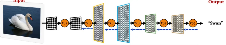
In Fig. 2.5, there are two parts: (i). Feature extractors - the input data goes through several convolutional layers to extract progressively more complex and ab-stract features, (ii). Classifiers the densely connected layers, and objective functions. TheFeature extractorsthat map the raw data to a transformed feature space, then ascore function that maps the extracted features to class scores, and finally aloss functionthat evaluates the relationship between the prediction and the ground truth numerically. Thus, the CNN algorithm casts this as an optimization problem in which it will minimize the loss function through backpropagation aka backpropagation (BP) with respect to the parameters of the score function.
based on the same principles to ensure some degree of shift, scale, and distortion-invariant by using local receptive fields, shared weights, and spatial sub-sampling. It is achieved by having series of Conv layers with interspersed pooling (Pool) and ReLU layers followed by two or three FC top layers while the last layer being a Softmax classifier [64], [72], [132]. Besides that, the network architectures are as a rule-of-thumb parametrized to be large and regularized during training using dropout [134]. It is has been empirically proven that the representation depth is beneficial for the classification accuracy, and that state-of-the-art performance on various data-sets can be achieved through ConvNet architecture [76], [133] with substantially increased depth.
2.9.1
Convolution layers
The convolution or conv layers are the heart of CNN, which contain neurons that take their synaptic inputs from a local region of the input volume called local receptive field (i.e., the filter, interchangeably the kernel), whereby neurons detect local visual features: oriented edges, end-points, or corners. The weights of the convolution neurons within a feature map are shared, so the position of the local feature becomes less critical, thereby yielding shift invariant. The feature map of a conv layer w.r.t. filter ω, its associated bias b and input image/ patch (aka set of input activations)x is computed as:
C(m, n) =b+
K−1 X
k=0
K−1 X
l=0
ω(k, l)∗x(m+k, n+l), (2.17) where ∗ represents the convolutional operation. A sample feature map generation through conv layer is shown in Fig. 2.6.
2.9.2
Densely connected layers
Densely connected layers or commonly known as fully connected (FC) layers take flattened, i.e., 1D output activations of the previous layer (be it a convolutional, pooling, or fully connected) and connects it to every single neuron it activates. Thus, the FC layers are not spatially located (just one-dimensional vectors), which implies that there can be no convolutional layers once a FC layer is employed in the chain of CNN. It can be expressed as F C = f(matmul (input f lat, WF C) +bF C) which
Figure 2.6: Convolution feature map generation in LeNet5 [77].
batch of vectors and weight matrix (WF C), andbF C is the bias vector associated with
each output activations. FC layers are to support the final classification process as shown in fig. 2.7, where the Softmax function, σ(·) is given by (2.20).
(Image:https://www.tensorflow.org)
Figure 2.7: An example of top fully connected layer.
2.10
Activation function
(NN) can be referenced to the work of McCulloch and Pitts in late 1943 [90], where the activation function rectifies the input to either 1 or −1 if its value is positive or negative, respectively. However, in CNNs, it takes a real-valued input (generally, the value strengthen after the convolved feature summation as shown in fig. 2.6) and performs a mathematical operation to convert it to range of [0, 1]. Historically, the sigmoid function is a default choice; however, it has recently fallen out of favor and it is rarely ever used [123] due to its technical drawbacks. Besides the sigmoid function, there are several other activation functions in practice such as Tanh non-linearity (tanh), Rectified Linear Unit (ReLU), Leaky ReLU, Parametric ReLU, and Randomized ReLU.
2.10.1
ReLU
The rectilinear units or ReLUs are nonlinear activation functions generally used after convolutional operations. The ReLU can be formally defined as in (2.18) when taken a case where there are K number of anchor vectors, denoted by wk ∈ RN, k =
1,2, . . . , K. For a given inputx, the correlations withak and k= 1,2, . . . , K, defines
a nonlinear rectification to an output y= (y1, . . . , yK)T, where
yk(x,ak) = max(0,a T
kx)≡ReLU(a
T
kx), (2.18)
i.e., it clips negative values to zero while keeping positive ones intact. The benefit of ReLU is sparsity, overcoming vanishing gradient issue, and efficient computation than other activation units.
2.10.2
Sigmoid
The Sigmoid activation function, on the other hand, has output in the range [0,1] for an input x and it is defined by
f(x) = 1
1 +exp(−x). (2.19)
2.10.3
Softmax
The Softmax activation is defined as,
σ(z)j =
ezj
PK
k=1ezj
f orj = 1, ..., K (2.20)
where, z is a K-dimensional vector of arbitrary real values and the output σ(z) K-dimensional vector of real values in the range (0,1) that add up to 1 as the normal-ization happens via the sum of exponents term dividing actual exponentiation term forming a valid probability distribution. Thus, if the final layer at the end of a CNN
is aSoftmax classifier, then it yields the actual probability scores for each class label.
Some cases, the Softmax layer is modified to calculate the cross-entropy loss through taking negative logarithm on (2.20);
Lj =−log
ezj
PK
k=1ezj !
(2.21)
where the logarithm is actually base e (natural logarithm).
2.10.4
Batch normalization
The batch normalization operation has multifaceted benefits:
i. Reducing internal co-variate shift - During training, there is a change in the distribution of activation maps as network parameters are being tuned. Such condition challenges the learning, but the BN alleviate pressure by maintaining the mean and standard deviation of the activation close to 0 and 1, respectively.
ii. Effect of regularization - Since the batch of examples given in the training are normalized, it increases the generalization of the model. It is also claimed that BN allows to reduce the strength of dropout.
iii. Counterbalancing vanishing or exploding gradients - When the BN is located prior to non-linearity, it avoids an undesirable situation, where the training saturates areas of non-linearities, solving the issues of vanishing exploding gradients.
Mathematically it can be defined as follows. Let the output of a layer X∈RN,D,
where N is the number of samples available in the mini-batch and D is the number of hidden neurons, then normalized matrix ˆX is given as in (2.22) [63].
ˆ
X= pX−µB
where µB, σB2, and refer to the mean and variance of the mini-batch, and a small
value of 0.001 to prevent division by zero, respectively. Then the layer maintains its representational strength by testing the identity transform as:
y=γXˆ +β, (2.23)
where, β and γ are trainable parameters that are initialized with β = 0 and γ = 1, in this work. Note that, when β = µB and γ =
p
σ2
B+ Eqn. (2.23) returns the
previous layer’s activation map.
2.11
Long-short term memory
Long short-term memory or the LSTM NNs are the advanced version of the general recurrent neural networks (RNN). The LSTMs overcome the vanish and exploding gradient issues of general RNNs by using the Constant Error Carousel (CEC) cells that use an identity activation function. The LSTM-based NNs interconnect sequential memories both in the long and in the short term, which makes them apt architecture for time-dependent tasks, viz. handwriting recognition [111], speech/language iden-tification [45], robot control/localization [151], driver distraction detection [163], and action recognition.
In every iteration, an LSTM module updates the state parameters and outputs by controlling a hidden vector h given by (2.29) and a memory register vector m given by (2.28). The LSTM networks inherit the ability to learn short-term tempo-ral dependencies in sequences as Graves et al. [68] drive the associated parameter computation at an iteration step t, like:
gu =σ(Wuht−1+IuXt), (2.24)
gf =σ(Wfht−1+IfXt), (2.25)
go =σ(Woht−1+IoXt), (2.26)
gc= tanh(Wcht−1+IcXt), (2.27)
mt =gtmt−1+gugc, and (2.28)
ht= tanh(gomt). (2.29)
the gates gu,gf, go, and gc refer to the input gate, the forget gate, the output gate, and the cell gate respectively.
2.12
Transfer learning
The essence of CNN architecture is how precisely modeling raw data samples through multiple processing layers with non-linearities; when a deep CNN has many parame-ters, for instance, the AlexNet [72] contains more than 60 million parameparame-ters, making it powerful function approximator. Such, deep neural networks have demonstrated ro-bustness in visual-based classification, recognition, and detection. However, training these models requires, large amount of labeled data (for instance, 14,197,122 images, 21841 classes in ImageNet 2016, Sep.), because directly learning many such param-eters from small data-sets, which contain only a few thousand training images is hard [103]. At the same time, there is a need for a careful initialization for optimized and efficient training. Hence, to train CNNs using large annotated images require specialized hardware, for instance, the GPUs (good GPU would cost few thousand dollars), GPU programming skills, energy and time.
Figure 2.8: Block diagram describing transfer learning technique.
Thus, when the task in target domain is trained on different statistics than the source domain, but using the learned parameters of the source task, it is conceived
as transfer learning (refer Fig. 2.8). Here, the outcome of using TL is tri-fold: less
Chapter 3
Literate review
Recent state-of-the-art technology in transistor fabrication has driven the clock rate of Central Processing Unit (CPU) and Graphic Processing Unit (GPU) to reach super high frequency; thus, the computational speed of processors has enormously in-creased. Hence, it has paved the way for bigger available physical memory or Random Access Memory (RAM) and storage disk space in modern computers. Consequently, it has enabled application of computer vision technologies in several fields, such as Multimedia-based surveillance, Industrial Automation [82], Automotive, and Intelli-gent transportation systems. In such applications, the FGL module plays an integral role in guiding vision-based solutions to ignore unwanted region of a scene monitored by exploiting visual properties and shifting the attention to moving objects, such as running vehicles and walking people. It is crucial when it comes to priority spe-cific data compression on Terabyte (TB) size multimedia (mainly video) surveillance footage.
For example, consider Fig. 3.1, where (a) is an actual scene1, and (b) is the useful FG region, which is about 25 to 30% of the actual scene. This piece of
in-1 A scene in Railway data sequence downloaded from http://www.cs.cmu.edu/~yaser/new_backgroundsubtraction.htm
formation is valuable for a video compression algorithm so that it can use selective techniques to compress the FG and BG regions differently, whereby details of the useful FG region remain intact while the BG region experiences higher compression rate. Besides, once the FG objects/regions are well localized, the fruitful low-level visual cues of the current scene can be extracted, and it can be, then, employed for high-level analysis. The followings are few applications as the product of such high-level analysis: autonomous/intelligent driving [6, 170], object indexing and re-trieval [20,74,143], traffic monitoring (detecting, counting or tracking of objects) [167], human activity recognition (run, walk, jump, squat, etc.) [55], human-machine in-teraction (in general, human-machine interface- HMI) [46], moving object tracking (many live sports telecasting channels have adopted this) [184], scene classification, digital forensics [118, 157], image quality assessment [4, 28], and so forth.
Pixel-based
Region-based Hybrid
Sample-based Probability-based Subspace-based
Codebook-based Neural network-based
Figure 3.2: Categories of foreground localization algorithms.
The FGL algorithms and models can be categorized as the Venn diagram in Fig-ure 3.2. There are five categories:
1. Sample-based [11, 62, 137, 144, 146],
2. Probability-based [3, 34, 65, 139, 149, 158],
3. Subspace-based [10, 52, 102],
4. Code book-based [138, 164, 176], and
Then, all these five categories can be grouped into pixel-based, region-based, and the combination of the two strategies. The sample-based algorithms create a BG from the past set of N frames, i.e., for each pixel location there are N samples stored. If there arek number of pixels in the BG that have a distance smaller than a threshold τ to the incoming pixel, then the pixel is classified as FG. The probabilistic models work on the principle of stochastic process, like Gaussian mixture models (GMM) [3, 94] and Conditional Random Field (CRF)-based algorithms [187]. The subspace-based approaches perform a transformation of data to a subspace, such as Eigenspace or Principal Component Analysis (PCA)-based subspace. Then, they form a BG model using the subspace and estimate the FG. The Code-book generates a dictionary that consists of color, intensity, temporal features, or similar representations. Same properties of a new pixel are compared with the dictionary values to determine it’s status. The NN-based models are kind of generating a classifier through training to handle the segmentation task. The trained weights of a NN serve as BG model and can be updated to reflect the changes occurred in the scene. Here, a learning system, which formulates FGL as a structured input-output matching problem. Such models have gained their reputation after breakthrough performances in the ImageNet-Large-Scale Visual Recognition Challenge (ILSVRC). The NN-based techniques have been exploited for image semantics/ labeling [130, 178], medical image partitioning [109, 119], and recently for video FG segmentation [169] as well. The main challenges in CNN-based FG detection is that dealing with time-dependent motion and the dithering effect at bordering pixels of FG objects. We address these issues in Chapters 7, 8, and 9, by excogitating an encoder-decoder (EnDec) CNN-LSTM that utilizes ResNet [56]-like residual connections for lost feature recovery and LSTM units to handle spatiotemporal motion of FG objects. To facilitate the training process, we take advantage of intra-domain transfer learning.
3.1
Pixel-based background modeling
are chosen to represent the BG. Following the work of Stauffer and Grimson, sev-eral researchers in this domain have proposed various techniques in order to im-prove the statistical model. Among them, some researchers focus on techniques to update the model parameters, for instance, Zivkovic [186] implements an adaptive algorithm to choose a required number of Gaussian components per pixel and up-date the model parameters. Similarly, Dawei et al. [32] and Zhou et al. [182] take advantage of expectation-maximization (EM), k-means clustering, Kernel density es-timation (KDE) and Markov random field (MRF) for parameter updates and to refine the estimated FG respectively. Since the MRF-based FG refinement is an it-erative process, it generally consumes higher processing time. On the other hand, Yang et al. [160] utilizes a spatial relationship between neighboring pixels through a conditional random field (CRF), which influences the learning process of the GMM-based classification for in-door video segmentation. This model faces a significant toll in computational speed and implementation complexity. To address this issue, Mukherjee et al. [91] propose a wavelet-based decomposition and a variable number of clustering technique (referred as WavGMM hereafter). This approach decomposes the input scene into multi-resolution sub-bands so that useful features in different scales can be incorporated in the learning step as temporal data with the considera-tion that the sub-bands are relatively independent. At the same time, this method achieves better computational speed because the sub-bands are smaller compared to the original input image. Lee [78] proposes a technique to balance GMM convergence speed and stability through computing appropriate learning rate when parameters of a Gaussian are updated and integrates a Bayesian framework to isolate the most-likely BG Gaussian distributions and generate an intuitive representation of the believed-to-be-BG. This approach, however, falls into the cost of additional computation and updates.
Besides the GMM based approaches, Bayesian-based BG modeling frameworks also have frequently been adapted for BG-FG separation. In [113], Zhu et al. take a multilayered Gaussian distribution to initialize each pixel for dissimilar BG contents and a recursive Bayesian learning based on texture correlation to refine the detected FG. Likewise, Li et al. [79] use Bayesian decision rule that incorporates spectral, spatial, and temporal features to define BG. Vosters et al. [152] compute an Eigenstate model from a training set of BG images that are recorded under various lighting conditions from a fixed viewpoint and reconstruct a generalized BG.
![Figure 2.6: Convolution feature map generation in LeNet5 [77].](https://thumb-us.123doks.com/thumbv2/123dok_us/1345024.1167363/43.612.184.465.387.587/figure-convolution-feature-map-generation-in-lenet.webp)