Cliff edge seismic evaluation of stack structure using fragility analysis

ABSTRACT

The objective of this paper is to evaluate the cliff edge effect due to a seismic event for a stack structure, using fragility analysis. With similar configuration to a typical stack structure for of a boiling water reactor, this stack consists of a lattice support frame of rolled steel sections and an enclosed chimney of thin shell construction, located on the roof of a reactor building. Due to the amplification of the reactor structure and roof responses, the accelerations at the stack base are very high.

The cliff edge evaluation is based on fragility curves of the stack structure. The stack is comprised by two interdependent structural forms, ie. the lattice support frame and the chimney. The stack seismic capacity is described by the lowest acceleration value from either of the structural forms (corresponding to global failure of the lattice support frame, or the exceedance of the flexural capacity of the most stressed section of the chimney). With both interdependent structural forms modelled in a single finite element model, a pushover analysis has been undertaken with plastic hinges introduced into the model at discrete locations, both in the lattice support frame and the chimney. The interactions of both structural forms have been investigated and it was concluded that the chimney shell reaches failure before the lattice support frame. Based on the pushover analysis results, fragility curves of the stack structure are developed using modification of the approach as documented in EPRI TR-103959. Fragility curves are created at the confidence levels of 5%, 50% and 95%.

In summary, a set of fragility curves for the stack have been developed using pushover analysis, thus performing the cliff edge seismic evaluation with the determination of the limiting base acceleration at a given probability.

INTRODUCTION

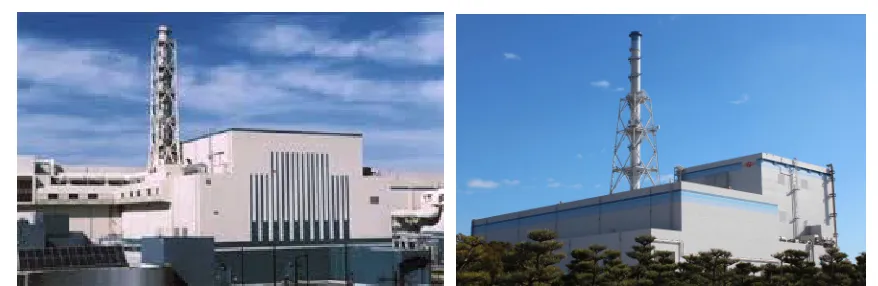
Figure 1: Stack Structures at Kashiwazaki-Kariwa & Tokai Daini NPPs (photos extracted from www.alamy.com)

As shown in Figure 1 above, the stack structure considered in this paper is typical of a boiling water reactor main stack, which consists of two main parts, the lattice frame and the chimney. The stacks often located directly on top of the reactor buildings’ roof which is beneficial from operations and flooding perspective, but not so from seismic perspective as it will sustains high amplifications. For the purpose of this paper, the stack is assumed to be located at the roof of a reactor building. The stack comprises two interdependent structural forms, ie. a lattice support frame and a chimney. Both interdependent structural forms modelled in a single finite element model, a pushover analysis has been undertaken with plastic hinges introduced into the model at discrete locations, both in the lattice support frame and the chimney.

The lateral load used in the pushover analysis is derived based on the dynamic response of the stack-lattice support frame analysed as part of the design process. In particular, the mass and the acceleration at specific locations of the stack derived as average of the maximum accelerations in these locations from a number of time-history analyses are used to calculate the load vector for the pushover analysis described in more detail in accompanied paper by Hadfield et al. (2017).

Damage accumulation over the structure is monitored and the deterministic seismic capacity is defined. The EPRI TR-103959, EPRI (1994) procedure is used as a basis to derive the median capacity and the uncertainty range used in the definition of the fragility curves.

PROBLEM DESCRIPTION

Figure 2. Figures should be centred and followed by a numbered caption.

FE MODEL

The pushover analysis is performed in SAP2000. The NASTRAN FE model described in Hadfield et al. (2017) is converted to an equivalent representative SAP2000 FE model. For purposes of the pushover analysis the Stack Shell is represented by equivalent line (frame) elements. Standard formulae are used to calculate the equivalent cross-section properties for the closed sections of the Stack Shell. A large Main Duct Hole typical of this kind of stack structure is included in the model as this create a potential weak spot to the chimney. This is included by reducing the cross-section properties for the open section. For reference purposes, the line (frame) elements representing the Stack Shell are referred to as the "Stack Shell frame elements" in the text below. The converted equivalent representative SAP2000 FE model of the Stack, showing the Lattice Support Frame and the Stack Shell frame elements, is illustrated below. The mass of the model is 184.9t.

Plastic hinges are introduced into the SAP2000 FE model at discrete locations. The plastic hinges simulate the development of yielding and load re-distribution in the structure with increased pushover load, thus effecting the non-linear pushover analysis study. Axial hinges, simulating tensile yielding and buckling when in compression, are placed in the Lattice Support Frame elements (vertical columns and diagonal bracing) since the main load resisting system against overturning is via axial loads in these members. Flexural hinges are placed in the Stack Shell frame elements since the load resisting system against overturning is in bending.

Axial Plastic Hinges for the Lattice Support Frame

Figure 3. Representative SAP 2000 FE model of the Stack.

The yielding force in axial tension FT is computed as:

y

T AF

F = . (1)

where A is the net cross-section area; Fy is the yielding strength.

The ultimate force in axial compression FC is computed as:

cr

C

A

F

F

=

.

where

(

)

= _{y C}

cr F if

F λc

λ

(3) or

5 . 1 ,

. 877 . 0

2  >

  

 

C y C

if

F

λ

λ

and

E F

r L

K y

C .

. .

π

λ

where A is the net cross-section area; Fy is the yielding strength; Fcr is the buckling strength; λC is a

slenderness parameter; E is the elastic modulus; r is the radios of gyration; K is the buckling shape coefficient to account for support conditions (assumed as 1); L is the member length

The axial force capacities are calculated using the expected (best estimate) yield strength of Fye=400MPa.

where Z is the plastic section modulus; Fye is the expected yielding strength; P is the axial force in the

member at target displacement in non-linear analysis (axial force under gravity load used in this study as no significant difference in axial load and no significant effect on the section capacity); Pye is the expected

yield axial force of the member

The yield rotation θY capacity is calculated as:

        − = ye c c ye Y P P I E l F Z 1 . . . 3 . .

θ

where Z is the plastic section modulus; Fye is the expected yielding strength; P is the axial force in the

member at target displacement in non-linear analysis; Pye is the expected yield axial force of the member;

E is the elastic modulus; Ic is the second moment of area 3 is a constant for cantilever end conditions.

Table 5-7 of FEMA 356 is used instead Table 9-7 of ASCI 41-13 because the specification for circular hollow tubes in the FEMA document can be directly applied for the above mentioned analogy to the stack section. FEMA 356 Table 5-7 differentiate the circular hollow tubes only based on the dimeter to thickness ratio that is compared with a parameter derived from the yielding strength. ASCI 41-13 Table 9-7 use more complex equations to differentiate between slender and stocky pipe elements which include the stiffness K of the member and the length L. However, since the structural system of the stack is fundamentally different from that of a brace, using more complex equations to differentiate between slender and stocky element will not will not lead to any benefits. In addition, the selected values from FEMA 356 Table 5-7 are more conservative, which in this case is more suitable due to the unclear real failure behaviour. For consistency, the deformation capacities of the axial hinges described above are also based on FEMA 356 Table 5-7.

LOADING AND PUSHOVER ANALYSIS

For purposes of applying load in the pushover analysis, a '1g' load vector is first created, for both the X EW and Y NS horizontal directions. This '1g' load vector represents a series of lateral static forces to be applied to the Stack to simulate the seismic load such that this '1g' load vector can be scaled up in the pushover analysis so that the base shear at failure can be used to calculate the limiting base acceleration level Ad. The '1g' load vector forces are applied at the lateral support positions where the Lattice Support

Frame connects to the Chimney. The '1g' load vector (as indicated by '1g') is created such that the base shear, Vb, is equal to what would happen if an inertial load of 1g were placed on the structure (Vb is therefore equal to the Total mass of the Stack x 1g, ie. 184.9t x 9.81ms-2 = 1813kN).

aAC at the support positions (where Stack is connected to the Lattice Support Frame) is based on an

average of the maximum accelerations of each support position. Since that the accelerations are extracted from another seismic analysis, consideration is therefore given to the actual dynamic seismic response of the Stack, as well the influence of the dynamic response of the building structure (in which the stack is located on) in both directions.

Then, the extracted seismic accelerations, aAC, and the mass of the Stack at each support position, mL, are

used to calculate the corresponding base shear, VbAC, ie.:

AC AC

L

AC

m

a

F

Vb

=

Σ

.

=

Σ

where, FAC is the lateral force at each support position due to the extracted seismic acceleration aAC.

Next, the acceleration at each level, a, for the '1g' load vector is calculated, using the ratio of Vb (1813kN) to VbAC to scale the seismic acceleration, ie.:

AC AC

a Vb

Vb

a= × (9)

Finally the static lateral force at each level, F, for the '1g' load vector (where F = Vb = 1813kN) is calculated by multiplying the mass at each level, mL, by a, ie.:

a m

F = _L× (10)

Based on the above, the values of ZPA at the reactor structure roof are calculated to be 0.48g and 0.59g. This means that if the R/B roof ZPA was increased to 1g then the value of the base shears would be 1g/0.48g x 1813kN = 2.08 x 1813kN = 3793kN X EW and 1g/0.59g x 1813kN = 1.69 x 1813kN = 3078kN Y NS (this is important in establishing the value of Ad). Graphical representation of the tabulated load vectors is given in the figure below. It is seen that the load vectors in the X EW and Y NS directions are different. The Stack is roughly symmetrical but the X EW input acceleration time history has differing magnitude and frequency content from the Y NS – thus the values of aAC differ and therefore so

does the calculated load vector for each direction.

10.3 25.8 41.3

0 200 400 600 800

L e v e l a b o v e b a s e [ m ]

Load vector [kN]

1g X EW

1g Y NS

Figure 4. Load vectors in X EW and Y NS direction, equivalent to ‘1g’ ZPA at stack base.

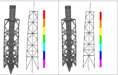
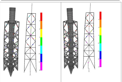
relate to stages of failure in the formation of the plastic hinges. It is observed that the Chimney reaches failure before the Lattice Support Frame. The structural capacity in the Y NS direction is lower than in the X EW direction due to the more unfavourable load vector in the Y NS direction (see Figure 2). Note that even though the large Main Duct hole near the base is located on the +Y north, face, this hole does not govern the cliff-edge capacity as both the Stack Shell failures and Lattice Support Frame failures begin at the top of the structure and progress downwards

Figure 6. Lattice Support Frame failure mode in X EW (left) and Y NS direction (right). 0 2000 4000 6000 8000 10000 12000 14000 16000 18000

0.00 0.25 0.50 0.75 1.00 1.25 1.50 1.75

B a se S h e a r V b p [ k N ]

Displacement [m]

X EW Base Shear vs Top Displacement

F-d X EW Stack Shell Failure Lattice Support Frame Failure

0 2000 4000 6000 8000 10000 12000 14000 16000 18000

0.00 0.50 1.00 1.50 2.00 2.50 3.00 3.50 4.00

B a se S h e a r V b p [ k N ]

Displacement [m]

Y NS Base Shear vs Top Displacement

F-d Y NS Stack Shell Failure Lattice Support Frame Failure

Figure 7. Capacity curves in X EW and Y NS direction.

The base shears corresponding to a ZPA at the R/B roof of 1g (denoted here as VbZPA_1g) are 3793kN X

EW and 3078kN Y NS. Using the Vbp values from the above figures from the pushover analysis, the limiting base acceleration level Ad can be determined by considering the ratio of Vbp to VbZPA_1g, ie. how

much more than 1g at the base can the structure withstand before failure. The value of Ad (in g units) for

The safety factor is taken as 1.00 for purposes of this study. This is a conservative measure since it implies that there is no inherent over estimate of the value of Ad derived from the pushover analysis. The

value of Ad (with F for Am), serves as input to the fragility analysis. Fragility curves are developed by

adopting the approach in EPRI document TR-103959 in order to account for specific details of the Chimney and Lattice Support Frame of the Stack. The specific details for the various factors which affect the slope of the fragility curve are determined accordingly based on experience on similar structures and not discussed in this paper.

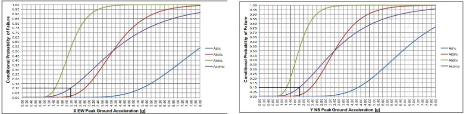
Fragility curves are developed, inputting the values of Ad, then Am, and adopting the approach in EPRI

document TR-103959. Fragility curves are created at the confidence levels of 5%, 50% and 95%, and also the composite curve (Acomp) which uses βC as an SRSS of the βr and βu values. Using the composite

curve, the X EW value of AL(10) is established as 2.18g and X EW value of AL(10) is established as 1.82g

(indicated by the black box on the Acomp fragility curve).

Figure 7. Fragility curves in X EW and Y NS direction.

CLIFF EDGE EFFECT EVALUATION

The fragility analysis is used to determine the lower limit of 10% confidence of median ground acceleration, AL(10), as per recommendation of ASCE 43-05 (ASCE, 2005). As described above the AL(10)

value in the X EW direction is 2.18g and the corresponding AL(10) value in the Y NS direction is 1.82g.

Table 1: Tables should be centred and preceded by a numbered caption.

DBE ZPA, m.s-2 _{1.5 DBE ZPA, m.s}-2

X EW Y NS X EW Y NS

11.1 5.79 1.70g 0.89g

Considering the AL(10) values from the fragility analysis, it is observed from the above table that the AL(10)

values in both directions exceed the maximum 1.5DBE values, ie. 2.18g>1.70g in the X EW direction and 1.82g>0.89g in the Y NS direction. It is therefore confirmed that there is significant seismic margin for the Stack and that there is not a disproportionate increase in risk from a seismic event of greater magnitude than the DBE.

CONCLUSION

A pushover analysis is used to derive the deterministic seismic capacity of a stack-lattice support frame structure. The deterministic seismic capacity is then used in fragility analysis that is based on modified EPRI TR-103959 approach adjusted to incorporate the specifics of the studied structure. The fragility analysis is used to define the seismic acceleration at stack base corresponding to the 10% confidence of the median capacity. This acceleration is then compared with the acceleration corresponding to the 1.5 DBE in order to confirm the absence of a cliff-edge effect just beyond the design basis. The presented study confirmed that there is a significant seismic margin for the Stack and that there is not a disproportionate increase in risk from a seismic event of greater magnitude than the DBE.

ACKNOWLEDGEMENTS

The work presented herein would not be completed without the support from Hirokuni Ishikagi-san of Hitachi-GE, of which we are extremely grateful.

REFERENCES

ASCE/SEI 43-05 (2005), Seismic Design Criteria for Structures, Sstems and Components in Nuclear Facilities, American Society of Civil Engineers.

ASCI/SEI 41-13 (2014), Seismic Evaluation and Retrofit of Existing Buildings, American Society of Civil Engineers.

EPRI TR-103959, (1994), Methodology for Developing Seismic Fragilities, Electric Power Research Institute

FEMA 356 (2000), Prestandard and Commentary for the Seismic Rehabilitation of Buildings, , Federal Emergency Management Agency.

Hadfield J., Tan M., Gumley R. and Y Nitta (2017), “Design Optimisation of Stack Using Time Domain Seismic Analysis”, 24th Conference on Structural Mechanics in Reactor Technology SMiRT24, Busan, Korea - August 20-25, 2017.