Application Interference in Multi-Core Architectures: Analysis and Effects

PhD Dissertation

International Doctorate School in Information and Communication Technologies

Department of

Information Engineering and Computer Science University of Trento, Italy

Application Interference

in Multi-Core Architectures:

Analysis and Effects

Alexandre Kandalintsev

Advisor:

Prof. Renato Lo Cigno

Universit`a degli Studi di Trento

Abstract

Clouds are an irreplaceable part of many business applications. They pro-vide tremendous flexibility and gave birth for many related technologies – Software as a Service (SaaS) and the like. One of the biggest powers of clouds is load redistribution for scaling up and down on demand. This helps dealing with varying loads, increasing resource utilization and cutting down electricity bills while maintaining reasonable performance isolation. The last one is of our particular interest.

Most cloud systems are accounted and billed not by useful throughput, but by resource usage. For example, a cloud provider may charge according to cumulative CPU time and/or average memory footprint. But this does not guarantee that the application realized its full performance potential because CPU and memory are shared resources. As a result, if there are many other applications it could experience frequent execution stalls due to contention on memory bus or cache pressure. The problem is more and more pronounced because modern hardware rapidly increases in density leading to more applications are co-located. The performance degradation caused by co-location of applications is called application interference.

In the following part we present a method of ranking of virtual machines according to their average interference. The method is based on analysis of performance counters. We first launch a set of very diverse benchmark programs (to be representative for wide range of programs) one-by-one to-gether with all sorts of performance counters. This gives us their “ideal” (isolated) performances. Then we run them in pairs to see the level of in-terference they create to each other. Once this is done, for each benchmark we calculate average interference. Finally we calculate the correlation be-tween the average interference and performance counters. The counters with the biggest correlation are to be used as interference estimators.

The final part deals with measuring interference in production environ-ment with affordable overhead. The technique is based on short (in the order of milliseconds) freezes of virtual machines to see how they affect other VMs (hence the name of method – Freeze’nSense). By comparing the performance of the VM when other VMs active and when they frozen it is possible to conclude how much it looses in speed because of sharing hardware with other applications.

Keywords

Contents

1 Introduction 1

1.1 Clouds under the hood . . . 3

1.2 Cloud Economics . . . 5

1.2.1 Why Clouds . . . 5

1.2.2 Why not Clouds . . . 8

1.3 Application Interference . . . 9

1.4 Motivation . . . 14

1.5 Research Objectives . . . 17

1.6 Structure of the Thesis . . . 19

1.7 Topics outside the scope . . . 20

2 State of the Art 23 2.1 Monitoring and On-the-Fly Profiling . . . 23

2.2 Performance Modeling . . . 28

2.3 Task-aware Scheduling . . . 30

3 Modeling Tasks Inter-Core Interference 35 3.1 Introduction . . . 35

3.1.1 The Benchmark Programs . . . 36

3.2 Problem Statement . . . 40

3.2.1 A Simple Experiment . . . 40

3.4 Performance Measure . . . 46

3.4.1 The Metric . . . 46

3.4.2 Accuracy and Overhead . . . 47

3.5 Model Validation . . . 48

3.5.1 Hardware Configurations . . . 48

3.5.2 Measurement Methodology . . . 49

3.6 Results and Analysis . . . 50

3.6.1 Digging Inside the Model . . . 52

3.6.2 The Two-Core Machine . . . 54

3.6.3 Intel W3670: The Six-Core Case . . . 54

3.6.4 Effects of Prefetching on Intel W3670 . . . 54

3.6.5 AMD FX-8120: The Eight-Core Case . . . 55

3.6.6 Improving the Precision . . . 56

3.7 Obtaining Model Parameters . . . 57

3.7.1 Direct Measurement . . . 57

3.7.2 Task Classification . . . 57

3.7.3 Low-level Resource Utilization . . . 58

3.7.4 On-line Tuning . . . 58

3.8 Conclusion . . . 59

4 Ranking VMs by their interference 61 4.1 Introduction . . . 61

4.2 Methodology . . . 62

4.2.1 Hardware Performance Counters . . . 63

4.2.2 Virtual Machines Profiling . . . 64

4.3 Experimental Study . . . 64

4.3.1 Testbed . . . 64

4.3.2 Benchmarks . . . 65

4.4 Performance Results and Analysis . . . 66

4.4.1 Analysis of different HPCs . . . 70

4.4.2 Lessons Learned . . . 76

4.4.3 Conclusion . . . 76

5 Freeze’nSense: Isolated Performance Sampling in a Shared Environment 79 5.1 Introduction . . . 79

5.2 Notation and Terminology . . . 82

5.3 Performance Isolation and Monitoring . . . 83

5.3.1 Symmetric Multiprocessing System (SMP) Open Issues 84 5.4 Methodology . . . 86

5.5 Implementation . . . 88

5.5.1 Benchmarks and Workload . . . 88

5.5.2 Performance Sampling Issues . . . 89

5.6 Results . . . 92

5.6.1 Freezing Validation . . . 92

5.7 CPU Load Balancing . . . 97

5.8 Conclusions and Discussion . . . 100

6 Conclusion and the Road Ahead 103 6.1 Future Research . . . 104

A Vocabulary 107 B Research Hiccups and Dead-ends 111 B.1 Importance of Storage . . . 111

B.2 Looping programs . . . 112

B.3 Unexpected Load Variation . . . 114

List of Tables

1.1 Memory access times (in ns) in a four CPU system. Num-bers represent how fast a CPU on row n can access memory

of another CPU on column m. . . 11

3.1 Rrmse accuracy of our model compared to the linear

predic-tion in different test scenarios for the two-core E7600 CPU. 51 3.2 Rrmse accuracy of our model compared to the linear

predic-tion in different test scenarios for six-core Intel W3670 CPU with enabled and disabled hardware prefetcher (HWP) and

Adjacent Cache Line Prefetch (ACLP). . . 51 3.3 Rrmse accuracy of our model compared to the linear

predic-tion in different test scenarios for eight-core FX-8120 CPU

with different cache control settings. . . 52 3.4 Performance penalty (percentage) for simultaneous task

ex-ecution on Intel E7600 CPU. . . 53

4.1 Performance degradation for concurrent execution of VMs

running the benchmarks on ARM Exynos reported in percents. 67 4.2 Performance degradation for concurrent execution of VMs

4.5 Correlation between interference, sensitivity and HPC. P-value is the probability that results are statistically

insignif-icant (null hypotesis), less is better. . . 73 4.6 Performance comparison of AMD FX and ARM Exynos

platforms1. . . 75

List of Figures

1.1 Load variation over 24h on Moscow Internet Exchange Point

(MSK-IX). The gap between day and night is up to 8x. . . 2

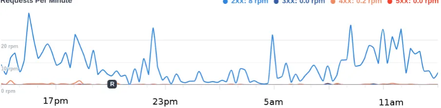
1.2 Load variation (in requests per minute) over 24h onCoDesign. io. “2xx” indicates normal server responses, “3xx” for redi-rects, the rest are for different types of errors. “R” label on X axis means there was a software update (“release”), it has

no special meaning in this context. . . 2

1.3 Good cloud: money saved on up-front investments helps

growing the business. For illustrative purposes only. . . 7

1.4 Two different scenarios: when clouds accelerate business de-velopment and when they don’t. Good clouds reduce up-front costs on infrastructure and maintenance, allowing to put saved money into business development (upper picture). Bad clouds: consider switching to a private cloud if your cloud provider charges too much (lower picture). For

illus-trative purposes only. . . 10

1.5 How far memory latency lags behind CPU performance. . 11

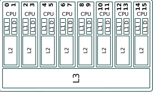
1.6 Inside Intel Xeon E5-2630 v3: every CPU core has two threads of execution (Hyper-Threading), “private” L1 and

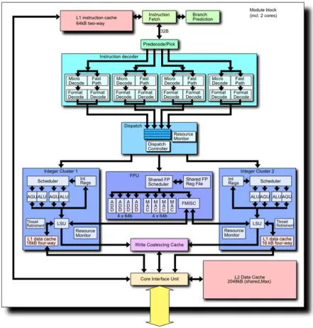
1.7 An AMD’s two-core “bulldozer” module. Picture shows that not only caches, but other CPU units can also be shared: FPU, instruction decoder, branch predictor, and thelike. Shared blocks aim at increasing average block utilization

and save some silicon area and power. . . 13 1.8 Performance scaling of SDAGP on AMDFX-8120 increasing

the number of parallel instances; the gap between the two

is due to shared hardware resources. . . 14 1.9 Current and future Internet traffic trends as seen by Cisco. 15

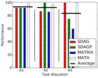
3.1 Performance of four benchmark programs in three possible

allocations A1, A2 and A3. . . 41 3.2 The effects of HWP and ACLP on the per-core performance. 55

4.1 Ranking process at a glance. . . 63 4.2 Software architecture of the experiments. . . 66 4.3 Four cases of interference for ARM Exynos: no interference

(only NGINX is running), negative interference (NGINX runs with INTEGER), medium interference (NGINX with

WORDPRESS) and strong (NGINX with MATRIX). . . 72 4.4 Execution profiles of benchmarks running on ARM Exynos.

Benchmarks are arranged according to theirinterference

fac-tors. . . 74

5.1 Performance scaling of SDAGP on AMDFX-8120 increasing the number of parallel instances; the gap between the two

is due to shared hardware resources. . . 81 5.2 Applications profiled in isolated (no other core is loaded)

and shared environments (the other cores are used too): the gap shows how large the difference can be (CPU: Xeon

5.3 Intel Xeon: estimate of ζb(i) when tasks runs alone in the

CPU and when the environment is frozen; tm =100 ms in

the upper plot, tm = 10 ms in the lower plot. . . 93

5.4 Intel Xeon: Reducing tm to the limit: estimate of ζb(i) for

tm = 10, 5, 2, and 1 ms; tsleep is reduced to 50 ms. . . 94

5.5 AMD FX: Reducing tm to the limit: estimate of ζb(i) for tm

= 10, 5, 2, and 1 ms; tsleep is reduced to 50 ms. . . 96

5.6 AMD FX: empirical pdf of ζb(i) estimates in isolation and

with Freeze’nSense for NGINX and BLOSC for tm = 2 ms. 96

5.7 ARM Exynos: estimate ofζb(i) when tasks runs alone in the

CPU and when the environment is frozen; tm =100 ms. . . 97

5.8 Distribution of performance improvement usingFreeze’nSense to decide Virtual Machine (VM) relocation. . . 98 5.9 Distribution of performance improvement of VMs relocated

by Freeze’nSense. . . 99

B.1 CPU and DISK load variation over 24hours for linux.org.

Chapter 1

Introduction

What makes cloud computing so attractive? Deploying applications of al-most any size and complexity is easy as never before. Cloud adopters do not need to concern about resources, scalability and reliability: these prob-lems are solved by the cloud provider. Clouds also fostered two business models previously unseen, or rarely used in IT: Pay-As-You-Go (PAYG) and Everything-as-a-Service (XaaS).

Pay-as-you-go frees cloud customers from upfront costs on infrastruc-ture. Before clouds, resource provisioning was a difficult tasks for many services because of variability of the load. For example, the day/night traffic variation can be a factor of 10 [29]. This means that the full compu-tational power is needed only during peak hours. As a result, many systems are underloaded most of the time and unused resources are just wasted. Fig. 1.1 shows the daily variation of traffic on MSK-IX, Moscow Inter-net Exchange Point; higher traffic corresponds to higher loads of servers. Fig. 1.2 shows backend load (in requests per minute) of CoDesign.io; the load changes from almost zero up to 30rpm.

CHAPTER 1. INTRODUCTION

Figure 1.1: Load variation over 24h on Moscow Internet Exchange Point (MSK-IX). The gap between day and night is up to 8x.

CHAPTER 1. INTRODUCTION 1.1. CLOUDS UNDER THE HOOD

makes it hard to deal with unpredictable spike loads. For most Internet services significant load fluctuations is more than normal, and this rendered most resources allocated statically unused at least half of the time. This underutilization is not just bad on initial expenses on equipment. Main-tenance costs (energy, cooling, spare parts) are also higher, significantly raising the Total Cost of Ownership (TCO).

XaaS is the further evolution of the cloud concept: not only hardware resources, but software and services can be rent on PAYG principles. It may take many forms and shapes, but, in general, it is something hosted remotely and available through some sort of remote API. Example XaaS: software-as-service – libraries and applications that integrate into other services or to be used alone – Google Translate, Travis CI (continuous integration service), Adobe Creative Cloud (Photoshop and other famous Adobe products) and even YouTube (though it is free for most users). It can also be a storage-, database- and even algorithm-as-a-service. The key aspect of of such services, besides ease of use, is (almost) zero support costs because it is a service provider’s responsibility to keep it up and running.

In this Chapter we fist discuss the rationale behind the success of clouds and how they are organized. Then we introduce the problem of resource management in the clouds – application interference, and our motivation. Then we present the structure of the thesis and topics that are covered in this work.

1.1

Clouds under the hood

1.1. CLOUDS UNDER THE HOOD CHAPTER 1. INTRODUCTION

level, but deeper inside; it is in the management plane.

Cloud resources must be well tracked and accounted for. The cloud provides customers with dynamic resource allocation: if some resources are not immediately needed they are put back to the resource pool. And vice versa: more resources are readily available if required. This provides customers with dynamic sizing of applications that may rapidly shrunk or expand depending on the demand.

Underneath of almost any cloud is resource virtualization. Applications no more run on bare hardware, they run in virtual containers of some kind: Virtual Machines (VMs). A VM mimics a physical node and it is almost indistinguishable from real hardware till it comes to scaling. VMs bring the following properties: a) multiple VMs can be collocated on the same node b) dynamic resource “sizing” c) isolation (problem with one VM does not propagate to others) d) relocation (they can be moved from one node to another). The ability to co-locate means denser packing: two or more customers can be put on the same server if resources allow. Dynamic sizing allows for scaling explained earlier. Isolation guaranties that security is not compromised, i.e., the vulnerability of one application cannot be used to gain access to other applications. Finally, relocation means VMs can be moved between the nodes without interruptions, also enabling seamless maintenance. This again helps scaling: applications are distributed to provide hardware footprint adequate to the load.

There are two approaches to provide scaling for applications. The first one relies on dynamic resource provisioning. Every VM is given the min-imal portion of resources required to serve the load. Underutilized VMs are shrunk, overloaded VMs are given more resources. If a VM does not fit the node it is relocated to another node with enough resources.

CHAPTER 1. INTRODUCTION 1.2. CLOUD ECONOMICS

vice versa: if the load is not enough to keep all VMs busy, VMs in excess paused or shut down and the load is redistributed. This method requires an external load balancer for load distribution.

In practice, these two approaches are often combined. For example, Amazon micro instances1 always provide a small baseline performance. In addition to that, micro instances that do not fully use their share are given “CPU credits” that can be used to deal with spike loads, backups or periodic activity. The peak performance can be 5 times higher the baseline.

1.2

Cloud Economics

“There is no Cloud. It’s just someone else’s computer.” (c) Internet folklore

“I don’t understand what we would do differently in the light of Cloud Computing other than change the wording of some of our ads.”

(c) Larry Ellison, former Oracle CEO

Depending on the use, clouds can be a project accelerator or a money black hole. On the strong side of clouds are ease of use, scalability, relia-bility, usage-proportional pricing, (almost) zero initial investment.

The downsides are potential privacy and legal issues, price benefits di-minish as the project scales up, vendor lock-in, and the exposure to the cloud provider failures. Here we quickly discuss factors to consider before giving clouds a green light.

1.2.1 Why Clouds

One of the most attractive cloud features is ease of use and access. Most cloud providers have nice and simple web interfaces allowing for easy

1.2. CLOUD ECONOMICS CHAPTER 1. INTRODUCTION

figuration of most common deployment scenarios. This straight-forward approach eliminates many risks associated with infrastructure setup: an improperly-configured infrastructure is an easy victim for hackers [68].

Common maintenance burden is also much easier with clouds. This often eliminates the need for dedicated infrastructure workforce, saving headcount for projects.

Scalability. For a rapidly growing company it can be difficult to scale IT infrastructure accordingly. This is less the case with cloud providers who do a number of steps to ensure their scalability. First, big “cloud” datacenters are built in areas where they can be easily expanded or there is enough place for more datacenters. Second, there is a good practice of choosing datacenter places where electricity and thick Internet links are not an issue. As a result, commercial clouds are much better ready for expansion than a typical private infrastructure. And because of their scale, they can sustain enormous spikes of load that would normally kill a typical private cloud.

With on-premises infrastructure it is also easy to mispredict the load. Companies overestimating their growth would waste their money on exces-sive infrastructure capacity. Underestimating the growth is also dangerous because not every infrastructure can be easily expanded. For example, once the datacenter is full there is no physical place put more hardware. Or the datacenter can be capped by power and cooling capabilities.

Pricing and minimal initial investment. PAYG allows paying only for consumed resources. Although this may not hold true for larger instances (discussed later), it is a money-saving option for projects not requiring lots of resources. But even for larger cloud installments it may worth using clouds because of larger gross margins: companies prefer to put money into growth rather than own infrastructure because this is more profitable in the long run [74]. Fig. 1.3 illustrates this.

CHAPTER 1. INTRODUCTION 1.2. CLOUD ECONOMICS

Efficiencies

Value Services Revenue

Profit Margin

Profit Margin

Ability to Sell Annuity Services

Sourcing “Long Tail”

Time Price/

Cost

$

Figure 1.3: Good cloud: money saved on up-front investments helps growing the business. For illustrative purposes only.

as never before, and often can be done with a few clicks in a browser. In fact, many well-known Internet services (like Dropbox, Netflix, Airbnb and many others) are built on top of other services.

Reliability. Comparing to a single-server deployment, a proper cloud has two big advantages. First, there are always spare resources to deal with hardware troubles. Second, storage is often network-enabled, eliminating the need to transfer user data between servers in case of migration. This helps relocating user from one machine into another in case of, e.g., failure or malfunction. Some providers even have live migration.

QoS. Clouds normally have 24x7 support and rapid incident response. This is useful for small companies that cannot afford covering non-working hours with on-call support.

1.2. CLOUD ECONOMICS CHAPTER 1. INTRODUCTION

be challenging and expensive. But sometimes it is possible to rent a private cloud that already meets the requirements.

1.2.2 Why not Clouds

Clouds are not always attractive, sometimes they may be undesirable or illegal to use.

Privacy and Trust. Cloud users give full access to their data to cloud providers; they do not have any control of what the provider does with it [46]. If the provider’s security is breached it can potentially affect all customers.

Legal issues. Not all data can be put into the cloud. For example, healthcare data is very restricted in Europe by “EU data protection regu-lation”. This makes impossible to use public clouds for many applications dealing with personal and sensitive data.

Pricing for large instances may be less fair. Cloud bills include fees for both hardware and services. As the scale grows the service “overhead” may outweigh PAYG benefits. Sometimes prices for large or dedicated instances are unjustified: for example, Amazon charges $2 per hour for each region of presence (“availability zone”) when it comes to dedicated hardware2. That is $2∗24h∗365d = $17.5k/year per region and does not include any computational resources.

Latency. Cloud services may not be close to customers and to each other. Building responsible applications in the cloud from elementary building blocks (frontend, backend, database, authentication, file storage, etc) can be a real problem because these blocks may not be in close proximity. The author had once to solve problems with poor application performance. It turned out, round-trip time to the database was too high for applications sending many SQL queries sequentially.

CHAPTER 1. INTRODUCTION 1.3. APPLICATION INTERFERENCE

Ownership. Cloud users are normally not in charge of everything. If something goes wrong or there is a lack of functionality customers can only complain and hope to be heard.

Vendor Lock-in. Most cloud providers have competing set of services, but each uses its own API and implementation. As a result, it is hardly possible to migrate from one provider to another without a big headache. This is especially true for storage and databases: different providers have different features and performance. For example, Amazon provides “cloud” databases based on Oracle, PostgreSQL and MySQL, while Google Cloud supports only MySQL. This also complicates the interoperability between different vendors.

All in all, clouds are a considerable choice for startup companies because they accelerate growth. For mature companies clouds are less attractive because costs savings are less pronounced. These two faces of clouds are on Fig. 1.4. We now move to more technical discussion on one important aspect of life of applications in clouds.

1.3

Application Interference

1.3. APPLICATION INTERFERENCE CHAPTER 1. INTRODUCTION

Leveraging Speed and Cost

Faster rate of cost reduction

Faster time to cost reduction

Adoption

of OPEX based Services

Adoption of Rapid Dev/Test/Deploy Lifecycle Total Cost

of Ownership

Traditional

Cloud TCO

Time $

(a) Clouds help returning on investment by lowering TCO. OPEX (OPerational EXpense) – money spent for keeping business running. Cortesy of The Open Group.

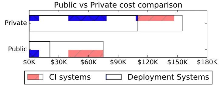
$0K

$30K

$60K

$90K $120K $150K $180K

Public

Private

Public vs Private cost comparison

CI systems

Deployment Systems

(b) Bad cloud: at some scale and “steady state” of business supporting own infrastructure is cheaper. Source: [60].

CHAPTER 1. INTRODUCTION 1.3. APPLICATION INTERFERENCE

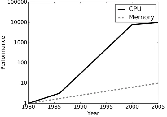
1980 1985 1990 1995 2000 2005 Year

1 10 100 1000 10000 100000

Performance

CPU

Memory

Figure 1.5: How far memory latency lags behind CPU performance. Source: [42].

CPU 0 1 2 3

0 136 194 198 201

1 194 135 194 196

2 201 194 135 200

3 202 197 198 135

Table 1.1: Memory access times (in ns) in a four CPU system. Numbers represent how fast a CPU on row n can access memory of another CPU on column m. Source: [87].

latency is far behind typical clock cycles of modern processors.

1.3. APPLICATION INTERFERENCE CHAPTER 1. INTRODUCTION L2 L1 D L1 I 0 1 CPU L2 L1 D L1 I 2 3 CPU L2 L1 D L1 I 1 0 1 1 CPU L2 L1 D L1 I 1 2 1 3 CPU L2 L1 D L1 I 1 4 1 5 CPU L2 L1 D L1 I 8 9 CPU L2 L1 D L1 I 6 7 CPU L2 L1 D L1 I 4 5 CPU

L3

Figure 1.6: Inside Intel Xeon E5-2630 v3: every CPU core has two threads of execution (Hyper-Threading), “private” L1 and L2 caches, and one big L3-cache shared between all cores.

Not only caches are shared, but many other “CPU building blocks” are shared as well. Fig. 1.7 shows the internal architecture of a two-core module of the AMD Bulldozer CPU Family. Apart from caches, module’s cores share instruction decoder, branch predictor and Floating Point Unit (FPU) block3.

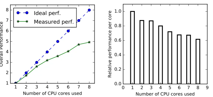
Fig. 1.8 highlights the problem. We launched one to eight instances of one machine learning tool [70] that performs comparisons between tree structures. The computing node was based on FX-8120, an eight-core CPU from AMD. If we take the speed of the first instance as 1, two instances show a total performance of 1.8. As the number of instances grows the total performance keeps increasing less than linearly. This means that every next CPU core contributes less and less to the total performance. With all cores active, the per-core performance is just ∼ 60% of what was seen when only one core was active (clearly, adding more cores to this

3_{We do not mention other shared units like instruction fetcher, instruction decoder or resource}

CHAPTER 1. INTRODUCTION 1.3. APPLICATION INTERFERENCE

1.4. MOTIVATION CHAPTER 1. INTRODUCTION

1 2 3 4 5 6 7 8 Number of CPU cores used 1

2 3 4 5 6 7 8

Overall Performance

Ideal perf.

Measured perf.

0 1 2 3 4 5 6 7 8 9 Number of CPU cores used 0.0

0.2 0.4 0.6 0.8 1.0

Relative performance per core

Figure 1.8: Performance scaling of SDAGP on AMDFX-8120 increasing the number of parallel instances; the gap between the two is due to shared hardware resources.

would be just a waste of silicon).

This performance degradation largely depends on the software running in the system (some programs tend to scale worse than others) and it is called application interference.

1.4

Motivation

Infrastructure bills can be enormously huge – $20B was spent just by Ama-zon, Google, Facebook and Microsoft in 2014. And, what is more frighten-ing, the Internet keeps growing (Fig. 1.9). Internetional Data Corporation (IDC) predicts worlwide spendings to reach $107B by 2017 [35]. With such high stakes efficiency plays a major role and every percent counts. The cost, demand, trends and environment – all these have become of great concern. However, despite growing demands, there are economical limits imposed on datacenters, they cannot grow infinitely.

CHAPTER 1. INTRODUCTION 1.4. MOTIVATION

2014

2015

2016

2017

2018

2019

0

5

10

15

20

25

30

Exabytes per Month

2.5EB

4.2EB

6.8EB

10.7EB

16.1EB

24.3EB

Figure 1.9: Current and future Internet traffic trends as seen by Cisco. Source: Cisco VNI Mobile, 2015 [44].

more computational power caused some drift towards new solutions like many-core systems, General-purpose Computing on Graphics Processing Units (GPGPU) systems, Application-Specific Integrated Circuits (ASICs) and Field-Programmable Gate Array (FPGA) solutions. Many-core and GPGPU systems impose significant restrictions on how a program should be written and work in order to fully utilize the advantages of the ar-chitecture. Most real-world programs cannot efficiently scale to tens and hundreds processing units [76].

ASICs are very expensive because it requires designing and manufactur-ing computer chips specific for a task. It is not just poor flexibility (a chip is normally designed to solve one and only one problem), but also enor-mous engineering efforts, huge costs of fabrication and long development cycles. This approach has currently no way to mass market.

1.4. MOTIVATION CHAPTER 1. INTRODUCTION

it could be beneficial to have custom (“soft”) computational architecture that can be tuned for the application. Unfortunately, FPGA accelerators are not available for cloud computing to date, although Intel aims at re-leasing their hybrid CPU+FPGA prototypes [37] in early 20174.

For all these reasons traditional datacenters remain here for long, and we need to pay special attention on their efficient usage. And that is what clouds are for – efficiency. Efficiency is achieved by careful tracking and accounting cluster resources. Resource management is at the very heart of every cloud: the quality of management defines performance, efficiency and robustness.

Thus, Cloud Resource Manager (CRM) is a central part of any cloud stack. It performs monitoring, scheduling and accounting of cluster re-sources and it gives a single point of control for the whole infrastructure. Tasks are no more statically instantiated and assigned to computers, they are dynamically placed according to the load, Service Level Agreement (SLA) and priority. Having different priorities is useful for different com-puting models. For example, mission-critical applications may co-exist with normal and batch-processing applications. In this case CRM first ensures that there is always enough room for mission-critical applications. The rest is dedicated to normal applications. Any resource leftovers can be given to batch-processing jobs that can tolerate performance variability or even full eviction during peak hours.

But this flexibility is not granted, in large clouds CRM has to handle a lot of resources. Nowadays machines with tens of CPU cores and hundreds of gigabytes of RAM are readily available on the market5. The scale of modern datacenters has grown up dramatically, hundreds of thousands of

4

http://fortune.com/2015/11/18/intel-xeon-fpga-chips/, accessed: 2015-12-13

5_{Intel Xeon E7-8800 v3 has 18 cores supporting up to eight sockets, that is 144 cores (or 288 if counting}

CHAPTER 1. INTRODUCTION 1.5. RESEARCH OBJECTIVES

servers is not uncommon6. That is, a datacenter can have well over million cores, petabytes of memory and exabytes of storage. To this end, it is very important for a CRM to be very efficient because at this scale every percent of performance matters. One thing, however, is often overlooked.

A server is not just a sum of its resources because they are intercon-nected, particularly memory and CPU cores. This means that tasks can greatly affect each other within the same system. Therefore, a management system that considers task placement problem as a “multidimensional bin packing problem” misses a great optimization opportunity: jointly placing tasks in such a way that their interaction maximizes performance.

Apart from optimizing task placement for better performance there are other questions related to performance and efficiency. Does optimal task placement means optimal performance for every task or we sacrificing per-formance of some tasks in favor of others? Can we make slow tasks running faster? In a heterogeneous hardware environment, what hardware is better for a specific task and why? What factors affect system performance and hardware efficiency?

1.5

Research Questions and Objectives

In this thesis we focus on the following research questions. Interference

We discuss why tasks interfere each other, how to measure the in-terference and what can be done to minimize it. We also discuss how to identify tasks that create the most interference and what placement schemes can help reclaiming lost speed.

6

1.5. RESEARCH OBJECTIVES CHAPTER 1. INTRODUCTION

Hardware efficiency

Same programs may show very different performance on differ-ent hardware platforms. Moreover, depending on the settings, applications may show quite different performance even on the same platform. We discuss the effects of hardware settings (like prefetching, memory frequency, etc) and even provide clues on choosing hardware platform (Intel, AMD, ARM) and a quick com-parison of ARMv7 and AMD Bulldozer platforms.

Task Classification

A cloud may run hundreds of thousands of tasks and measuring interference between all of them can be problematic. Fortunately, many tasks show similarity and we can exploit this to manage them in groups. In this work we will find out how we can identify such groups.

On-the-fly profiling

CHAPTER 1. INTRODUCTION 1.6. STRUCTURE OF THE THESIS

1.6

Structure of the Thesis

Chapter 2 gives an overview of state-of-the-art. It mainly consists of four sections. The first one is devoted to methods of monitoring and profiling of applications in the cloud. The second section is about performance modeling and interference prediction. Then we discuss modern algorithms for resource allocation and scheduling.

Chapter 3 presents a CPU performance model that takes interference into account. The model is based on the idea that the interference between any two applications is proportional to the time they run together. Thus, the total performance is the sum of isolated performances of all tasks minus the sum of all pairwise interferences.

Chapter 4 shows a simple method for ranking tasks according to aver-age interference they create. The performance model from the previous chapter requires an interference coefficient for each pair of tasks. Measur-ing them is impractical because for N different tasks we would need to measure N2 coefficients. But we can infer coefficients by sampling hard-ware performance counters (performance sampling). The problem is that performance samples do not provide interference characteristics directly, we obtain these by using statistical analysis. There is one drawback: the method requires performance samples not affected by interference because interference greatly affects them in an unpredictable way. This means that while sampling there should be one and only active application running in the system – the application we deriving interference characteristics for. This is fine for research work or profiling a limited set applications, but becomes impractical for anything serious. Fortunately, we effectively ad-dressed this issue in Chapter 5.

degrada-1.7. TOPICS OUTSIDE THE SCOPE CHAPTER 1. INTRODUCTION

tion can be very high, making it hard to guess if insufficient performance is due to the interference or problems on the application side. This approach eliminates uncertainty by providing accurate estimation of isolated perfor-mance. It works as following. Before taking a performance sample of the application in question, we temporary freeze all other applications in the system (hence why it we call it Freeze’nSense). Then we take a sample and unfreeze the system. The frozen phase no need to be long, often 10ms or less is enough. Short and fixed duration guaranties small and predictable overhead.

Chapter 6 concludes the thesis with a brief discussion of what is done, what is left to be done and future plans.

1.7

Topics outside the scope of the thesis

The focus of this work is the study and analysis of task interference on CPUs. The following topics are strictly related to cloud management and performance, but they are not addressed in this thesis.

CHAPTER 1. INTRODUCTION 1.7. TOPICS OUTSIDE THE SCOPE

name Xeon Phi7 is yet to come. They also, while mimicking the tradi-tional Intel’s architecture, quite depart from mainstream CPU computing and require using special programming tools to get full advantages of the architecture [69].

I/O issues. Storage, networking and other I/O are big topics on their own and are not part of the thesis. We do not study interference induced by, e.g, shared storage.

Precise simulation. We also did not aim at precise performance pre-dictions, our work is to steer CRM, preferably in real time, trading accu-racy for speed. Therefore, we do not compete with detailed machine- and DC-level simulators.

Placement Algorithms. Full-fledged placement algorithms are also not part of the thesis. There are many well known and “approved” (e.g., multidimensional bin packing) approaches to this. However, we provide a few examples of task placement algorithms for demonstration purposes.

Data locality issues in Non-Uniform Memory Access (NUMA) systems. In large systems, just one memory controller is not enough to serve the needs of CPUs. For this reason every CPU normally has its own controller and local memory, forming a so-called “NUMA domain”. From a program perspective there is no “domain boundaries” because hardware takes care and transfers data between CPUs transparently. But inter-domain transfers are expensive because they involve at least two CPUs (or more if it is needed to maintain cache coherency) and cross-domain links [63]. Therefore, the closer data is to the CPU the better the perfor-mance. Proper resource allocation place significant role in NUMA systems, but it is to some extent orthogonal to interference analysis.

7_{The project was started in 2009 and changed many names since then: Larrabee (supposed to work}

Chapter 2

State of the Art

2.1

Monitoring and On-the-Fly Profiling

Most of resource management algorithms consider CPU cores as unified resources adding performance in proportion to their number. That is, a six-core CPU to be three times faster than a two-core CPU running at the same frequency. In reality the performance gain may vary due to the subsystems shared between cores. These subsystems can include CPU caches, memory bus, I/O lines, instruction decoders, branch predictors, computational units and other components. Therefore, under heavy load it is unlikely to see a linear gain in performance when adding more CPU cores. In fact, an increase the number of cores can even degrade VM performance for up to 50% due to the inter-VM interference [96, 9].

2.1. MONITORING... CHAPTER 2. STATE OF THE ART

if their applicability is fare more specific compared to the methodology we propose, which is instead very general.

The most obvious way to profile the interference experienced by an application is to run it alone and compare its performance in isolation with its performance in a shared environment [49, 62]. This approach can be considered a benchmark, but it is not feasible as a production means. First, extra hardware resources are required. Second, given the enormous number of different applications and their specific customization, repeating the measurement for each of them is cumbersome and time consuming. If the spare hardware is limited, then the profiling cycle is also very long as all the different applications must be loaded and measured on the spare hardware. A long cycle may prevent a timely and efficient identification of bottlenecks, because applications can change their behavior in time.

A different perspective is represented by a cluster-wide massive data collection [95]. The idea is to collect performance statistics from different instances of the same application. If the statistical properties of the appli-cation are known or can be inferred with some techniques then the method-ology can identify instances that are under-performing. The approach is suitable for very large installations running many (stochastically) identical instances of the same application, while it fails for single and unique in-stances, but also for applications whose instances can be customized so that they are no more stochastically comparable. Applying this technique at the level of VMs is even more difficult as assuming identical configuration of VMs is far fetching.

per-CHAPTER 2. STATE OF THE ART 2.1. MONITORING...

formance only in a shared environment can be difficult, as the “ground truth” is missing.

However, there are techniques that can work in a production environ-ment without requiring many identical instances of the same application, and our work fits into this class.

In [65] Jia Rao et al. studied how pinning the threads of multithreaded applications to different cores influence the performance due to the data locality on NUMA systems [53]. Different thread-to-core mappings lead to different performance, but it is unknown in advance what mapping is the best. Thus, the proposal is based on random relocation of the threads to select the mapping that performs better. The relocation process is done in an initial time window during which the performance data of individual threads is recorded. At the end of the window the best allocation is chosen and the application continues to run steadily. The performance sampling is done with performance counters with sampling interval of 10 ms. The performance measure is based on the score derived from the number of L2-cache misses. The higher the score the more chances the thread is suffering. To accommodate changes in programs’ behavior the process of relocation must be repeated regularly. Unfortunately, the overhead of the relocation and measurement process is not negligible, specially when there are many threads in the system.

2.1. MONITORING... CHAPTER 2. STATE OF THE ART

default) parsed and the number of I/O operations for each VM is counted. Then, knowing the average CPU cost for each type of operation, it is possible to adjust the CPU consumption of each VM so they fit their performance limits or allocation targets.

Wood et al. proposed and implemented a gray-box monitoring for VMs [89]. In their system VMs are monitored both externally, using, e.g., statis-tics from the hypervisor, and internally, by running a small monitoring application inside each VM. The application exports performance statis-tics as it is seen from inside the VM. This helps to understand the way resources are consumed, as well as detect performance issues. The latter are detected by analyzing performance metrics exported by applications and the OS. If performance is not meeting the Quality of Service (QoS) constraints over a “sustained period” then there is a bottleneck and the VM is relocated to another machine with more resources available. The distinctive part of this work is the heuristic used to understand the trends in VMs’ behavior. For each resource there are two derived metrics calcu-lated over a sliding time window: distribution of the value and raw time series. The distribution is used by the migration manager “to estimate peak resource requirements and provision accordingly”. Time series show if a resource utilization rises, falls, or remains steady and they are used by the so called “hotspot detector” that drives the decisions to move the load from highly utilized servers to servers with lower load.

CHAPTER 2. STATE OF THE ART 2.1. MONITORING...

down we can conclude that the minimum efficient memory footprint is reached and the memory occupied by the artificial workload is the memory the database does not really need to run efficiently. The required CPU timeshare is calculated as the sum of individual timeshares of each database as if they were running alone. The required disk bandwidth is estimated from an empirical model based on multiple synthetic tests. The average probing overhead is claimed to be just 5%. The technique is aimed at large databases running directly on hardware; load balancing is done by moving tables between the databases.

Chopstix [19] is a Performance Monitoring Unit (PMU)-based tool for applications profiling. It has a traditional three-phase architecture (collec-tion → aggregation → analysis) with one distinctive feature: the perfor-mance sampling is probabilistic and done in adaptive intervals. That is, code functions that have less samples are more likely to be sampled [54].This greatly reduces the overhead of profiling and the size of collected data by reducing the sampling rate for the functions that already have a lot of samples.

In [31] researchers studied the possibility of predicting performance degradation using regression trees. They first analyzed the correlation between performance counters and the level of interference. This let them to drastically reduce the number of features: from 340 down to 19. Then they used WEKA [38] to build the regression tree. The tree was used for interference prediction of previously unseen workloads. The model was tested on two platforms (Intel and AMD) and showed the absolute error below 20% on the 80th percentile.

2.2. PERFORMANCE MODELING CHAPTER 2. STATE OF THE ART

In [32] authors proposed a hardware modification suitable for measur-ing performance degradation in Simultaneous Multi-Threadmeasur-ing (SMT) en-vironment. They upgraded PMU of DEC Alpha CPUs to categorize CPU cycles into three types: base (normal execution), miss event (cache misses and branch misprediction) and waiting (execution stalls). They also esti-mated the increase in cache misses due to resource sharing. The result were evaluated in SMTSIM simulator and showed average prediction errors of 7.2% and 11.2% for two- and four-thread SMT respectively. Unfortunately, modification of hardware is expensive, and such proposals rarely have their way into production.

2.2

Performance Modeling

Performance estimation tools for computing systems majorly fall into two categories: high-level models and precise cycle-accurate simulators [55]. The latter category provides nearly exact results at the cost of speed and complexity. Flexible simulators like [18] can not only predict the actual per-formance of the tasks but also give a hint concerning the bottlenecks. How-ever, simulation speed is a limiting factor. Execution inside fully fledged circuit simulators is too slow, making this technique useless for on-line performance prediction in cloud environments.

High-level models do not try to simulate the behavior of processors. The core of such systems is either an empirical or an abstract model (or a group of loosely coupled models) based on observations. High-level models neither interpret nor execute programs: they operate on traces and perfor-mance data obtained trough the normal execution of the programs. They try to predict the overall performance based on the past experience and interaction patterns that are mapped on the model parameters.

CHAPTER 2. STATE OF THE ART 2.2. PERFORMANCE MODELING

queueing network model of the memory architecture of CPUs, which was suitable for some classes of tasks.

Another simple performance model dedicated to threading applications and taking into account NUMA topology was proposed in [92]. The model shows a mere 15% error in general, which already enabled predictive man-agement.

The same authors in [91] explored the effects of dynamic page migration and its applicability for Gaussian 3, a multi-threading chemistry compu-tational tool, with a similar model.

A model that tries to predict the performance of threading applications and whose goal is the optimization of both thread and memory allocation is presented in [16], but the model goal is not on-line prediction, rather it is off-line understanding of different NUMA implementations and their threading performances.

The work presented in [11] discusses a hierarchical model used in Java-Symphony, a high-level framework for parallel and distributed systems viding transparent access to remote data as if the data were local. It pro-vides means and tools to build a hierarchical memory model that includes not only local resources (processors, memory bus, interconnections) but remote resources (remote machines and clusters) as well.

In general, all modern task schedulers are aware of data locality, CPU caches, and NUMA domains. For instance, Linux attempts to calculate the performance penalties for task migrations and memory allocations outside the current NUMA domain. This mechanism is usually tunable to ac-commodate different hardware systems, but does not contain a self-tuning feature.

2.3. TASK-AWARE SCHEDULING CHAPTER 2. STATE OF THE ART

initializing thread and the rest of the time the data is accessed from another thread possibly in another domain. The developed algorithm detects such cases and moves the data to the closest possible domain.

Thus, a large body of work exists on performance evaluation and perfor-mance impairments due to locality violation, unwanted tasks interaction, etc. However, a systematic study of how these performance impairments can be predicted and how they are influenced by different hardware is miss-ing and this is exactly the kind of tools that are needed for the management of large, heterogeneous facilities supporting cloud computing.

2.3

Task-aware Scheduling

In [73] authors present an interesting approach to optimize scheduling of multithreaded programs that extensively use shared memory. They found that there are cases when Linux cannot handle big shared data structures efficiently. It was proposed to split the load between multiple OS instances so each of them would be in charge of just a small portion of shared mem-ory. The optimization requires multiple OSes, a modified Xen hypervisor, and applications statically linked with a small helper library. The key ad-vantage of the technology is that, thanks to virtualized system calls and memory management, one process may span across multiple OSes. The resulting structure is called SuperProcess, and it is supervised by Virtual Machine Monitor (VMM). VMM manages system calls (including file sys-tem that appears to be transparently shared) and memory management so that all processes that form SuperProcess have a consistent view to the resources. The optimization framework was tested on two machines (16 core Intel and 48 cores AMD) with reported average speedups of 1.7x and 4x under full load.

pre-CHAPTER 2. STATE OF THE ART 2.3. TASK-AWARE SCHEDULING

sented in [83]. Cooperative programs inform the manager about resource policies they want and the manager dynamically adjusts their execution accordingly. Apart from CPU and memory, tracked resources include tem-perature, frequency, number of active threads or even memory prefetching. Such a rich set of monitored resources allows the manager to define mul-tiple global goals, such as maintaining the node power or cooling budget or aiming at best power efficiency. Programs may request more threads to be spawned when there are spare resources or adjust CPU limits ac-cording to the changing load. It was also shown that disabling prefetching when it does not help can save up to 12% of energy with speedup up to 8% comparing to when it is always enabled. The speedup by prefetching was determined by comparing the system performance with and without it (“start and stop” technique). The manager showed less than 3% overhead, worked on Linux and was evaluated on x86 and SPARC.

In [41] the authors studied two options for application scaling: more threads vs processes. The study performed on Lighttpd webserver and an eight-core system. It was found that, depending on the number of active cores, these approaches produce different results and none is the winner in general. Threads allow for some memory savings because they share com-mon data. But for this reason the performance degrades significantly when they spread over multiple NUMA domains: a) processors have to keep shared data in sync, and b) access to non-local data is much longer [81]. The best results are achieved by the hybrid approach when every CPU runs its own threaded instance of application.

2.3. TASK-AWARE SCHEDULING CHAPTER 2. STATE OF THE ART

task switching, cache displacement and longer scheduler queues1. For this reason high-load systems avoid spawning too many processes (and 8·128 = 1024 processes is a bit too much for an eight-core system).

ReSense [28] optimizes tasks placement according to their memory re-source consumption. It has two phases, offline and online, and uses perfor-mance counters to estimate usage of memory bus and caches, this is done in isolated environment on the target platform (offline phase). Then sensitiv-ity score is derived for each application. During the online phase ReSense optimizes task placement according to their sensitivity score. The opti-mization is to be repeated when the number of active threads is changed. The strong point of this work is the support of multithreaded programs. The proposed method also differentiates two levels (types) of resource con-tention: between threads of the same application and between different applications.

In [78] authors clustered threads based on their data sharing. If threads frequently access the same memory (at L2 cache-line granularity) and run on different CPUs they are to be placed together. But only if the CPU stalls are above the threshold, otherwise data sharing is considered a non-issue. Access patterns were detected with PMU counting for L1 data misses that were satisfied by remote L2 and L3 caches. The optimization could reduce sharing by up to 70% on the Power5 platform. The performance boost was more moderate – up to 7%, mainly due to the Out-of-Order (OoO) execution and thick inter-chip links.

Zhuravlev et al. [97] developed a “contention-aware scheduling” algo-rithm that balances miss rates among the Last-Level Caches (LLCs). The balancing was done according to estimated mutual interference via the cache. They evaluated six different approaches for interference estimation,

1_{Although the modern Linux scheduler CFS uses red-black tree instead of plain queues ([88]) the}

CHAPTER 2. STATE OF THE ART 2.3. TASK-AWARE SCHEDULING

the most promising was based on stack distance profiles [24]. Unfortu-nately, due to the implementation difficulties this algorithm was not used for online scheduling. They used heuristics based on cache miss rates of individual applications that also showed good estimations. Reported av-erage improvement was 20% with up to 50% for individual applications. The scheduler showed to be good in reducing performance variation be-tween different program executions. The best improvement was observed when memory intensive applications neighbored with non-intensive.

Cache Coloring (Partitioning)

These techniques are a little bit apart from what we are doing, but they serve the same purpose: optimize data access in multicore environments. Therefore, it is worth mentioning them.

Common Instruction Set Architecture (ISA) do not allow for cache con-trol overriding, i.e., a program cannot tell the CPU the importance of different pieces of data. A not-so-uncommon situation is when live data is constantly evicted while access-once data may be held for longer. This is because cache metadata (cache tags and flag bits) may not have enough information to understand complex data access patterns. Notwithstanding that, knowing how the CPU uses caches a programmer may enforce desired cache store policy by placing data in specific addresses.

2.3. TASK-AWARE SCHEDULING CHAPTER 2. STATE OF THE ART

possible to partition the cache between the tasks so they will not overlap in the cache. A few works that tackled this issue.

In [77] authors introduced an OS-level cache partitioning. It was done through a modified process of physical page allocation that required no changes in applications. The algorithm managed L2 cache on IBM Power5 and gave up to 17% speedup. The cache was not divided into equal por-tions, but dynamically partitioned according to the needs of applications. To achieve this, the performance curves (instruction stalls and L2 miss rates vs partition size) were obtained for every target process. Then each process was given a piece of the cache to minimize total (system-wide) instruction stalls. The cache could be partitioned up to 16 equally-sized blocks because the target CPU uses the last 4 bits of the page address to determine the data location. It was observed that most applications are comfortable with just two blocks (256KB) of L2 cache. This is where the speedup came from: only the applications that could really benefit from larger portions of the cache were given them. The run-time performance statistics was obtained with performance counters.

There are some inherited problems peculiar to these techniques. First, different CPUs have different cache configurations, algorithms must adjust to the running hardware. Second, the CPU’s own resource planners may interfere.

Chapter 3

Modeling Tasks Inter-Core

Interference

3.1

Introduction

The first step to solve a problem is to recognize it, and devise a first, simple conceptual model that represents it. Inter-core interference has been recognized as a problem in computation since many years [48, 90, 23, 30, 92, 82], but very often either disregarded or dismissed as a minor problem, compared to others [47, 72, 80, 33]. We have discussed the state of the art on data-center management and we have also discussed some works that do represent in some way inter-core interference, but we think a more specific model is needed.

This Chapter introduces a simple, first order model that captures the influence of one task running on a core on another task running on another core. Advanced modeling techniques like [22, 8, 61] can be used in future works to refine the model once the key features of interaction are better understood with simple models.

3.1. INTRODUCTION CHAPTER 3. MODELING...

questions: i)how a given set of tasks performs simultaneously, andii)what tasks are better neighbors one another.

The contribution of this Chapter is thus twofold. First of all, we show and highlight to what extent tasks running on different cores of the same CPU can affect each other performance, casting light in a phenomenon that is qualitatively well known, but quantitatively largely ignored in data center management. Second, we analyse to what extent a simple model that is suitable for on-line training and tuning can be used as a prediction tool to enhance CRM systems.

The remaining is organized as follows. Sect. 3.2 introduces the problem with some initial and simple measures of performance and efficiency and introducing our terminology. Sect. 3.3 contains the major contributions, formalizing the problem and describing the behavioral model. Sect. 3.4 describes the metric we use to evaluate models of performance prediction. Sect. 3.5 presents methodology we use for the model validation. Sect. 3.6 provides a deep analysis and discussion of the results. Sect. 3.7 describes how the parameters of the model can be obtained and Sect. 3.8 concludes the chapter summarizing the contribution.

3.1.1 The Benchmark Programs

Before going further it is worth describing benchmark programs we use for experiments. For the sake of convenience, we describe the whole set of benchmarks present in the thesis. In this Chapter only SDAG, SDAGP, MATRIX and MATH are used (described below).

The choice of benchmarks was not random. To make our studies more comprehensive, we chose programs of different and distinctive classes with different memory footprints, cache-awareness, utilization of memory band-width and CPU arithmetic units. Here they are:

randomly-CHAPTER 3. MODELING... 3.1. INTRODUCTION

generated square matrices. It is based on Basic Linear Algebra Sub-programs (BLAS) library – an industry standard for such kind of computation. BLAS takes roots from late 1970-x when first specifi-cations were published.

We used to use a quite trivial Python script with some NUMPY routines (another golden standard for such kind of computations) but it showed great variability in results due to intensive garbage collection, randomised data placement and other factors we could not account for. So we replaced NUMPY with BLAS rewrote program in C.

2. SDAG: a machine-learning program from natural language process-ing domain [70]. The program uses Support Vector Machines (SVM) to build compressed syntactic trees from text. It written in C and uses state-of-the-art processing techniques and manual optimizations allowing it work very fast. Particularly, the memory layout is very cache friendly.

3. SDAGP: a machine-learning program from [70]. It mostly resembles the previous one, but with one difference: it does not attempt to split the training set into smaller chunks for parallel processing, the data processed in whole. For the algorithm it is not a big deal, but for the CPU this means much bigger active dataset. As a result, there is much higher pressure on caches and the memory bus.

3.1. INTRODUCTION CHAPTER 3. MODELING...

is a simple program the sequentially compresses and decompresses 3e6 numbers (of type float64) evenly distributed between 0 and 100. 5. FFMPEG: a set of libraries and programs for decoding, encoding and re-encoding multimedia streams. It is one of two tools (another one is GStreamer) extensively used for video processing. If an appli-cation does something with audio or video, chances are one of these libraries is used. As a benchmark we used slightly different scenar-ios. For this Chapter it was a transcoding of a 1280X720@25Hz video (obtained from a camcoder) to a higher compression (lower quality). For Chapter 4 and Chapter 5 we scaled FullHD trailers down to 720p (Terminator 2 and Avatar trailers correspondingly).

6. NGINX: (pronounced as “engine x”) a very popular webserver that, as of November 2015, serves 27.9 millions of sites [7] all over the world. It uses asynchronous architecture and heavily tunned for performance. With NGINX a single machine (though a powerful one) can handle hundreds of thousands simultaneous connections with some tens of thousands active. Typically, it is used as a reverse proxy for slow applications or a load balancer.

7. MATH: a small ad-hoc C program performing basic integer com-putations. Ages ago, when floating point computations were expen-sive, people used to use so-called “fixed-point arithmetic” because it was much faster. Nowadays it less likely to find an application that would do intensive integer computations because floating point is fast enough for most applications (and even if not it is possible to use GPU for acceleration). Yet, to have a comprehensive set of benchmarks, we decided it is worth including a program that would do basic arithmetic with integers and just it, nothing else.

CHAPTER 3. MODELING... 3.1. INTRODUCTION

9. WORDPRESS: a popular web publishing platform serving more than 60 millions websites [26]. It is not the only of its kind, but it is the most used one. Technically it consists of two big components: the application code and the database. As database we used MySQL because it is the most popular choice for such kind of services. The benchmark is just to access the main page. Nonetheless this cre-ates serious load for the server (mostly by PHP, much less by the database). We did not used any PHP accelerators or any caching, this a pure “dynamic” load.

3.2. PROBLEM STATEMENT CHAPTER 3. MODELING...

3.2

Problem Statement

One of the most important role of a CRM is to minimize the amount of equipment to be provisioned (i.e., maintained active) in order to maintain the SLA (Service Level Agreement) with customers. This is achieved by dynamically assigning tasks to hardware resources, i.e., consolidating the load into a smaller number of nodes when the system is over-provisioned and increasing the resources when it is approaching overload. In both operations the capability to predict performance is fundamental to achieve efficiency and minimize reconfigurations.

Most CRM algorithms assume that the load of nodes is fully determined by resource requirements of the tasks, and the performance scales linearly with the load; in particular tasks running on different cores are considered independent. If, for instance, two tasks require one CPU core each, the CRM can put them together on any node having two cores free, assum-ing they will run without interaction. In the next section we show this assumption is wrong.

3.2.1 A Simple Experiment

As discussed in the introduction, most CRMs today consider tasks assigned on different cores and CPUs independent one another: is this assumption reasonable?

CHAPTER 3. MODELING... 3.2. PROBLEM STATEMENT

A1

A2

A3

Task Allocation

0

20

40

60

80

100

Performance

SDAG

SDAGP

MATRIX

MATH

Average

Figure 3.1: Performance of four benchmark programs in three possible allocations A1, A2 and A3.

We consider all the three possible assignments (distributions) of tasks to cores: as cores are identical the other three permutations of four tasks in two cores maps to the first three.

The results are presented on Fig. 3.1. The performance is normalized with respect to the same tasks running alone on the computer. As we see, the performance never reaches the maximum even in the best distribution. Indeed, the task assignment has a huge impact, lowering the average per-formance from roughly 95% to about 80%. What is worse is the fairness with one program (MATRIX), whose performance is nearly halved in one assignment.

3.3. INTERRACTION MODEL CHAPTER 3. MODELING...

instruction decoders and other circuits are often shared to increase their average utilization and to reduce the silicon area occupied. By assigning two tasks to the neighbor cores we can create a hidden bottleneck due to the shared usage of CPU subsystems (or to the other extreme speed-up the execution if the tasks share some data; more on this in Sect. 3.6).

A discussion on its own would be needed for hyper-threading and the related technologies, but this is beyond our scope.

3.3

A First Order Interaction Model

As proven by our simple experiment, the “load” of a cluster is not simply the sum of the loads of each running task as if it were alone, but it must take into account also the overhead induced by interaction of the tasks. We can treat the overhead as an additional load for the sake of performance prediction. With this simple observation in mind we derive a simple be-havioral interaction model with the assumption and notation introduced hereinafter.

Assumptions

CHAPTER 3. MODELING... 3.3. INTERRACTION MODEL

Notation

We define the task load Li = L(Ti) on a core as the time share required

by task i on the core. The per-core load is the sum of loads created by all tasks running on that core and is in the range [0,1]. The number of cores is N. We define the system load Lsys as a sum of loads of all CPU cores in

the system; it is in the range [0, N]. The pipe notation Ti|Tj means that

tasks Ti and Tj are running on different cores.

Let’s consider the following scenario. We have two tasks A and B run-ning on CPU cores 1 and 2 and exclusively occupying all CPU time. As we noticed, the joint performance in this case is less than what normally ex-pected, and thus we have an overhead that can be expressed as a parasitic load Loh_A|B, leading to a system load that can be expressed as

Lsys(A|B) = LA +LB +LohA|B (3.1a) Loh_A|B = βA|BLALB (3.1b)

where βA|B expresses the level of interference of the tasks A and B as

a function of the product of each task load. Remember that loads are represented by time shares, so we can imagine that the product of the time shares of two tasks represents the time during which the tasks actually interfere as they are running together on the cluster.

3.3. INTERRACTION MODEL CHAPTER 3. MODELING...

which is already quite complex [80].

The overhead function can be decomposed to represent the performance penalty for individual tasks:

Loh_A|B = βA→BLALB +βB→ALBLA (3.2)

This is useful, for instance, for real-time systems when we want to know how high-priority tasks are affected by the other non real-time tasks.

Formula (3.2) can be transformed into a matrix form, which will come very handy in the generalization of the model to multiple tasks and many cores. The tasks running on core i are represented by the vectorTi of loads

they generate. The values of the vector components are in range [0,1] with 0 meaning that the corresponding task isn’t scheduled on this core and 1 meaning it is using the core all the time. These vectors are sub-stochastic, meaning that the sum of their components is less or equal to 1. The matrix form of (3.2) for a two-core architecture two tasks A and B is:

βA→BLALB =

LA 0

βA→A βA→B

βB→A βB→B

! 0 LB (3.3a)

βB→ALBLA =

0 LB

βA→A βA→B

βB→A βB→B

! LA 0 (3.3b)

or in a compact and more general form:

Loh_1→2 = TT₁BT2 (3.4)

where B is the matrix of β-coefficients, T1 and T2 are the vectors of the

tasks running on cores 1 and 2 respectively and Loh_1→2 is the overhead that all tasks on core 1 impose the tasks on core 2.

Diagonal elements (βA→A, βB→B, . . . ) are of special interest. They tell

CHAPTER 3. MODELING... 3.3. INTERRACTION MODEL

cases. Knowing the overhead and using Amhdal’s law [15] we can estimate the scalability limitations of the system.

In order to generalize the model let’s consider the case of two cores and three programs (A, B, C); on the first core one copy of each program is running, while on the second core only the programs B and C are running, hence we have (TT₁ = |L1_A L1_B L1_C|T_{) and (T}T

2 = |0L2B L 2 C|

T_{). The program}

A isn’t launched on the second core and therefore its time share is zero in T2. The overhead created by core 1 tasks on core 2 is:

Loh_c1→c2 = βA→BL1AL 2

B +βA→CL1AL 2 C

+βB→BL1BL 2

B +βB→CL1BL 2 C

+βC→BL1CL 2

B +βC→CL1CL 2 C

= |L1_A L1_B L1_C|



 

βA→A βA→B βA→C

βB→A βB→B βB→C

βC→A βC→B βC→C

   0

L2_B

L2_C

= TT₁BT2

It is easy to see that (3.4) is a general representation of the overhead imposed by one core on another, regardless of the number of tasks per core. The description of the total overhead in an N-core CPU is given by the sum of all the overheads imposed by tasks of every core on every other core:

Loh_sys = Loh_c1→c2 +Loh_c1→c3. . .+ Loh_c1→cn

+ Loh_c2→c1 +Loh_c2→c3. . .+ Loh_c2→cn