Decrypting “Cryptogenic” Epilepsy: Semi-supervised
Hierarchical Conditional Random Fields For Detecting
Cortical Lesions In MRI-Negative Patients
Bilal Ahmed [email protected]
Department of Computer Science Tufts University
Medford, MA 02155, USA
Thomas Thesen [email protected]
Comprehensive Epilepsy Center, Department of Neurology School Of Medicine, New York University
New York, NY 10016, USA
Karen E. Blackmon [email protected]
Comprehensive Epilepsy Center, Department of Neurology School Of Medicine, New York University
New York, NY 10016, USA
Ruben Kuzniecky [email protected]
Comprehensive Epilepsy Center, Department of Neurology School Of Medicine, New York University
New York, NY 10016, USA
Orrin Devinsky [email protected]
Comprehensive Epilepsy Center, Department of Neurology School Of Medicine, New York University
New York, NY 10016, USA
Carla E. Brodley [email protected]
College of Computer and Information Science Northeastern University
Boston, MA 02115, USA
Editor:Benjamin M. Marlin, C. David Page, and Suchi Saria
Abstract
population. The lesion is detected by fusing the outlier probabilities across multiple scales using a tree-structured HCRF. The proposed method achieves a higher detection rate, with superior recall and precision on a sample of twenty MRI-negative FCD patients as compared to a baseline across four morphological features and their combinations.
Keywords: Conditional Random Fields, LOF, Focal Cortical Dysplasia, Epilepsy
1. Introduction
Epilepsy is a common neurological disorder, affecting approximately 1% of the world’s pop-ulation (Hauser and Hesdorffer, 1990). It is characterized by profound abnormal neural activity during seizures and inter-ictal periods. Uncontrolled epilepsy can have harmful effects on the brain and has increased risk of injuries and sudden death (Bernasconi et al., 2011). About one third of epilepsy patients suffer from treatment-resistant epilepsy (TRE); their seizures cannot be managed by medicine (Kwan and Brodie, 2000). Cortical malforma-tions, particularly focal cortical dysplasia (FCD) is recognized as the most common source of pediatric epilepsy and the third most common source in adults with TRE (Kuzniecky and Barkovich, 2001; Lerner et al., 2009).
Early detection and subsequent surgical removal of the FCD lesion is the most effective treatment to stop seizures and is often the last hope for TRE patients. A growing number of studies demonstrate that surgery is highly effective for FCD patients (Benbadis et al., 2003). However, the surgical procedure remains underutilized. One of the main reasons for this is that about 45% of histologically-verified FCD patients have normal MRIs (Wang et al., 2013). The chance of success for the surgical resection based on a visually detected lesion (MRI-positive) is 66%, which drops to 29% when the MRI is read as normal (MRI-negative) (Bell et al., 2009). Therefore patients who lack an MRI-visible lesion are less likely to be referred to specialized epilepsy centers by neurologists (Benbadis et al., 2003) likely because epilepsy specialists are reluctant to operate without a well-defined lesion (Tllez-Zenteno et al., 2005).
In this paper, we present an automated method for detecting FCD lesions using surface-based morphometry (SBM) (Dale et al., 1999) to extract the cortical surface from the T1-weighted structural MRI scans. The key advantage of using SBM is that the cortical su-faces of different individuals can be registered to an average surface allowing for point-wise comparisons between different individuals. The proposed method first applies a multiscale segmentation of the cortical surface and then combines the results via a hierarchical con-ditional random field (HCRF) (Reynolds and Murphy, 2007). Because we do not have accurately labeled training data, we cast the problem as a semi-supervised outlier detection task and thus we extend the HRCF framework proposed in (Reynolds and Murphy, 2007) to perform semi-supervised outlier detection. The resulting outlier regions (lesions), sorted by their probability and surface area, are shown to a team of radiologists and neurosur-geons who can combine the MRI lesion-detection results with other information such as the pattern of seizure onset and the patient’s intracranial EEG (iEEG) data to determine the final candidate resection zone.
that each pixel in the image have a label or that a bounding box around the object(s) of interest is provided. Consequently, the accuracy of the labels directly impacts the final performance of the HCRF. In this paper, we propose an extension of the HCRF-based image segmentation and object detection framework for problems in which pixel-level labels are not available. For our task, we are given the MRIs of patients and of normal controls, but information about which pixels form a lesion in the patient MRIs is either missing or highly noisy (Ahmed et al., 2015). Thus, we have a global label for each image indicating either that the image contains no lesions (healthy control) or that it contains one or more lesions (FCD patient). In Section 2 we explain in more detail why we cannot use the lesions/resection zones of previously treated patients as labels during training.
In a preliminary version of this work (Ahmed et al., 2014), we applied the proposed HCRF framework to both MRI-positive and MRI-negative patients using only cortical thick-ness as the feature of interest. Our preliminary findings showed that HCRF was able to achieve a higher detection rate with significantly higher precision and recall as compared to a recently reported semi-supervised approach (Thesen et al., 2011) and a human expert.1 The current work extends that body of work by evaluating the proposed method on three new morphological features. In addition we investigate different mechanisms of combining the detections produced by the different features to achieve higher detection rates. In our experiments we observed that it is not straightforward to combine the detections of indi-vidual features, because some of the features are noisier than others i.e., have a higher false positive rate than others. We show that this issue can be overcome by either using feature selection or changing the cluster ranking criterion. We provide extensive results on a larger set of patients2 as compared to our previous work, showing that feature selection can be used to achieve a high detection rate by appropriately tuning the ranking criterion.
The remainder of this paper is organized as follows. In Section 2 we briefly introduce SBM, the different morphological features that can be extracted within the SBM frame-work, and describe the current state of the art in lesion detection using SBM and its shortcomings. In Section 3 we detail how we pose the lesion detection task within the ob-ject detection/segmentation framework, where the saliency of the target obob-ject is defined based on its “outlier-ness”. We present different methods for combining the results of using four different morphological features in our proposed lesion detection framework. Section 4, provides the details of our ranking and evaluation methodology and it also provides an em-pirical comparison of our approach and a baseline approach across different morphological features and their combinations.
This work makes a significant contribution toward the detection of FCD lesions. Our empirical evaluation demonstrates that the proposed method was able to detect abnormal regions within the resection zones in a higher number of MRI-negative patients as compared to a baseline approach across four morphological features and their combinations. Not only was our method able to achieve a higher detection rate, it did so while achieving significantly higher precision and recall. Indeed, our 75% detection rate on the MRI-Negative patients
1. We omit the results of the blind comparison to a human expert in this paper. Interested readers can refer to (Ahmed et al., 2014).
2. The current sample has twenty patients, fourteen of which are retained from the previous study. In
Section 4 we exlain that the twenty patients comprise theentireset of MRI-Negative patients successfully
in our evauation dataset (compared to a human expert detection rate of 0%), suggests that this method can be used as an effective tool in the pre-surgical evaluation of TRE patients who are likely to undergo surgical resection; our method has started to be incorporated in the weekly meetings of radiologists and neurosurgeons to help identify the seizure onset zones in MRI-Negative patients. Thus, this work has the potential to increase the number of patients who are referred to resective surgery, and ultimately who are seizure free after surgery.
Our contribution to machine learning in addition to making progress on a challeng-ing and important application is a new method for uschalleng-ing HCRFs for binary object detec-tion/segmentation for which only image captions are available. The proposed method can be generalized for other data modalities such as time series data, where it can be used for time series segmentation. A caveat to this contribution is that the individual data (images/time series) must be able to be accurately aligned such that a one-to-one correspondence can be made between them.
2. Surface Based Morphometry
Surface based morphometry (SBM) provides the means to characterize and analyze the human brain by explicitly modeling the cortex using a suitable geometric model (Dale et al., 1999). The cortical surface represents the outer layer of the brain modeled as a folded two-dimensional surface in three-dimensional space. T1-weighted structural MRI scans are used to extract the cortical surface by delineating the boundary between the gray and white matter (Dale et al., 1999). This process is referred to as surface reconstruction, and involves a number of reconstruction and segmentation steps aimed at locating the gray/white matter boundary up to submillimeter accuracy (Fischl et al., 1999a). The reconstructed surface is represented as a triangulated mesh and at each vertex different morphological features are estimated to characterize the cortex. It should be noted that the spatial resolution of the reconstructed surface is different from that of the MRI volume.
This section introduces surface based morphometry. We first describe the different features that can be used to characterize the cortex that have been used for detecting FCD lesions. We also provide the related work where machine learning methods have been used in conjunction with SBM to detect FCD lesions.
2.1 Morphological Features
In this work, we use four morphological features to characterize the cortex:
1. Cortical thickness: represents the thickness of the cortex which is defined as the distance between the gray/white matter boundary and the outermost surface of the gray matter (pial surface). It is calculated at each vertex using an average of two measurements (Fischl and Dale, 2000): (a) the shortest distance from the white matter surface to the pial surface; and (b) the shortest distance from the pial surface at each point to the white matter surface.
interpolation of the images. The range of GWC values lies in [−1,0], with values near zero indicating a higher degree of blurring of the gray/white boundary.
3. Sulcal depth: characterizes the folded structure of the cortex. It is estimated by calculating the dot product of the movement vectors with the surface normal (Fischl et al., 1999a), and results in the calculation of the depth/height of each point above the average surface. The values of sulcal depth lie in the range [−2,2] with lower values indicating a location in the sulcus whereas higher values indicate a location on the gyral crown.
4. Curvature: Curvature is measured as 1r, where r is the radius of an inscribed circle and mean curvature represents the average of two principal curvatures with a unit of 1/mm (Pienaar et al., 2008). Mean curvature quantifies the sharpness of cortical folding at the gyral crown or within the sulcus, and can be used to assess the folding of small secondary and tertiary folds in the cortical surface.
Thesen et al. (2011) nominate cortical thickness along with GWC as the two most informative features for detecting FCD lesions in MRI-positive patients, using a vertex-based detection scheme. Similarly, Hong et al. (2014) identify GWC, cortical thickness and sulcal depth as being more sensitive to detecting FCD lesions in MRI-negative patients. However, they also note that most of the false positives detected using their proposed approach were largely caused by sulcal depth. The technical details of both these works are provided in the next subsection. In this study we use the four features described above, and also analyze different mechanisms to combine their detections in order to achieve higher sensitivity.
After surface reconstruction, different morphological transforms can be applied to reg-ister the cortical surface to a standard surface also known as a group-atlas. Registration is achieved by aligning specific sulcal and gyral patterns across the reconstructed cortical surfaces allowing for a more precise comparison of individual cortical structures across sub-jects (Fischl et al., 1999b). SBM has been used successfully for analyzing and detecting neurological abnormalities in various neurological disorders such as Schizophrenia (Rimol et al., 2012), Autism (Nordahl et al., 2007), and Epilepsy (Thesen et al., 2011; Hong et al., 2014).
2.2 Current Methods for Detecting FCD using Surface Based Morphometry
In this section we first define the related work with regards to automated techniques of FCD lesion detection. We then discuss the critical limitations of existing approaches. Most of the techniques reported thus far in literature deal either with MRI-positive patients (Besson et al., 2008; Thesen et al., 2011) or patients who were initially deemed MRI-negative during their preliminary radiological screening, but later their lesions were found to visible on MRI (Hong et al., 2014). As opposed to these studies, we evaluate our proposed methods on a sample ofpure MRI-negative patients whose lesions are not visible on their MRI.
vertex as being normal or lesional. Hong et al. (2014) developed a two-stage Fisher linear discriminant analysis (LDA) (Bishop, 2006) classifier to detect FCD lesions in patients who were radiologically classified as MRI-negative. Initially they train a vertex-level classifier that classifies each vertex on the reconstructed cortical surface as being lesional or non-lesional for both controls and patients. These detections are further refined using a second LDA classifier that is trained to distinguish between actual FCD lesions (detections made inside the manually traced resection zones of patients) and spurious lesional detections made on controls. The lesions for all the patients included in the study were ultimately found to be visible and were manually traced by an expert using texture-based maps. Thesen et al. (2011) use a semi-supervised uni-variate z-score based thresholding approach on registered SBM data of MRI-positive patients to classify each vertex as being lesional or normal, us-ing cortical thickness, GWC, curvature, sulcal depth and Jacobian-distortion, individually. They nominate cortical thickness along with GWC as being the most informative features for FCD lesion detection in MRI-positive patients.
These studies classify individual vertices of the cortical surface as lesional or normal, using labeled training data from MRI-positive patients and controls. There are four crucial issues that these studies fail to address:
(1) The goal of resective surgery is to remove the entire lesion. If any part of the lesion is left behind, the outcome will not be successful. This introduces label noise, because the expert-marked lesion can contain normal vertices; the margin around the lesion is marked in a “generous” manner so as to increase the chances of capturing the entire lesion. In our previous work (Ahmed et al., 2015) we used a stratified logistic regression classifier to detect lesions in MRI-negative patients. By manually reducing the resection masks for MRI-negative patients to correct for label noise we were able to achieve a detection rate of 58%, as opposed to 12% when the original resection masks were used as the ground truth. (2) These studies assume that individual vertices are i.i.d., completely ignoring the spatial correlation that exists between neighboring vertices. It has been shown in other domains such as object detection and segmentation in natural images, that modeling spatial correlations leads to superior performance (Reynolds and Murphy, 2007; Plath et al., 2009). (3) Vertex-based classification methods typically employ a post-processing method to reduce the false positive rate. In this strategy a portion of the vertices labeled lesional by the classifier are re-labeled as normal. This can be done by training a second-level classifier to classify the detected clusters as lesional or non-lesional (Besson et al., 2008; Hong et al., 2014). Similarly, different heuristics can also be used such as the surface area of the detected clusters (Thesen et al., 2011). Discarding any detected region based on its size or surface area can result in discarding the actual lesion or part of the lesion, because FCD can be located in any part of the cortex, is highly variable in size, and may occur in multiple lobes (Blumcke et al., 2011).
(4) Results are evaluated on MRI-positive patients, but the real challenge is to find lesions in MRI-negative patients.
using unsupervised segmentation of the flattened cortex that isolates regions of homoge-neous feature values. As the size of the FCD lesions has a wide range, using a single scale to isolate the lesion may not be effective. To minimize the chances of missing the lesion, we employ a multiscale strategy where the segmentation is carried out at different scales of varying granularity. The interplay between the patches obtained in this scale hierarchy is modeled as a tree structured HCRF, rooted at the most crude scale and having leaves at the finest scale. We fully exploit the spatial dependencies in the data by classifying image patches rather than by individual vertices, and furthermore larger spatial interactions are accomodated by explicitly modeling the dependencies using HCRF between image patches at different scales. Third, we define a ranking criterion which takes into account both the size and probability of a cortical region (cluster) that is labeled as being lesional. This ranking approach eliminates the need to post process the results, and provides a natural way of presenting the results to a radiologist to function as a focus of attention mechanism. Finally, we evaluate our approach on MRI-negative patients whose resections contained the primary FCD lesion, confirmed by a histological exam on the resected tissue. Since the pro-posed method is semi-supervised we use the z-score based approach (Thesen et al., 2011) as the baseline from which to contrast the performance of the HCRF method. Furthermore, the patients and healthy controls used in this work were treated and scanned at the NYU Comprehensive Epilepsy Center, where the z-score based method is currently part of the pre-surgical evaluation protocol of epilepsy patients. The next section describes the details of the HCRF construction and inference.
3. Hierarchical Conditional Random Fields
construction and inference of an HCRF for lesion detection. Subsequent sections provide the necessary technical and processing details involved at each step.
3.1 Adapting HCRFs for Lesion Detection
For FCD lesion detection, we have training data from MRI-negative patients who have undergone surgical resection and are seizure-free. The resected coritcal region, can be used to obtain vertex-level labels which can be used to train a classifier. However, as explained previously these labels tend to be highly noisy and using them to train a classifier will result in noisy predictions (Ahmed et al., 2015). To ameliorate this problem we extend the HCRF framework proposed in (Reynolds and Murphy, 2007) to perform outlier detection on registered image data. In contrast to the approaches mentioned previously, we cannot utilize vertex-level labels. Our proposed method works in a semi-supervised manner, where only global labels are available i.e., whether the cortical surface belongs to a healthy control or a patient. Thus, we define an FCD lesion as a region of the brain which is considered an outlier when compared to the same region across a population of normal controls.
The construction of the HCRF for FCD lesion detection involves the following steps (Ahmed et al., 2014):
1. Segment the cortex at multiple scales, to obtain image patches of varying sizes.
2. Assign an outlier score to each image patch by comparing it to the same cortical region across the control population. This one-to-one comparison is made possible by registering all the control’s and patient’s cortical surface to the same average surface.
3. Construct multiple HCRFs, one for each image patch obtained at the coarsest scale.
4. Run inference on the HCRFs to calculate the posterior probability at each node. The final lesion is detected by thresholding the posterior at the leaves.
We start by describing our approach to segmentation.
3.2 Segmentation
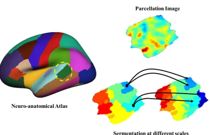
Figure 1: Constructing an HCRF using a standard neuroanatomical atlas (left), and a par-cellation image (top-right). Any morphological feature can be used to represent the image (the image is created using cortical thickness). At the bottom we have image patches obtained at two different scales using Quickshift. Each image patch on the coarser scale (bottom-left) becomes a root having children at the adjacent finer scale (bottom-right).
curvature, etc.), can be used to represent the intensity values in the resulting image. Figure 1 illustrates the overall HCRF construction process for a parcellation.
We use quick shift (Vedaldi and Soatto, 2008b) for unsupervised segmentation. One of the main advantages of using quick shift is that the number and size of segments need not be specified. Additionally, quick shift does not penalize for boundary regions, and produces a diverse set of segments having different shapes and sizes. It should be noted that any segmentation method can be used, as long as it has the ability to segment the image at different scales.
The standard quick shift algorithm is a fast mode seeking algorithm similar to mean shift (Comaniciu and Meer, 2002). It performs a hierarchical segmentation of the image, where the sub-trees represent image segments. It has two parameters namely the size of the Gaussian kernel (σ) used by a Parzen window density estimator, and the maximum distance (∆) between two pixels permitted while remaining part of the same segment. We vary the scale parameter σ to change the average size of segments, and set ∆ to be a multiple of
σ (Vedaldi and Fulkerson, 2008a). Thus, higher values of σ produce larger segments. By using different combinations of these parameters, we construct the scale-hierarchy which is the basic building block of the HCRF, as explained next.
3.3 Multiscale HCRFs
We model the joint prediction of these mutually dependent labels of all the patches using a tree structured HCRF. LetIpk+1 be an image patch at levelk+ 1, it has a parentIqk
at the immediately coarser level k, such thatIqk has maximal overlap withIpk+1 (Reynolds and Murphy, 2007). We find the index q as follows:
q:= arg max
q
|Ipk+1∩Iqk|
|Ik
q|
(1)
Each patch at the coarsest scale is the root of a tree having leaves at the finest scale. Therefore, the parcellation image is represented by a forest, where each tree is modeled as an HCRF, as shown in Figure 1.
CRFs model the joint conditional probability distribution of all the patch labels y =
(y1, . . . , yn) in the tree based on the values of the input morphological feature (x). Generally,
this can be written as:
p(y|x, θ) = 1
Z(x, θ)
Y
i
φ(yi|x, θ)
Y
i,π(i)
ψ(yi, yπ(i)) (2)
where, π(.) represents the parent patch, and Z(x, θ) is the normalization constant also called the partition function. φ(.) is called the node potential and represents the local evidence for the labelyi based on the observed datax. The edge potentials that model the coupling between adjacent labels are represented by ψ(.). As the graph is a tree we can efficiently calculate Z(x, θ) and the posterior probabilities of the patch labels at all scales using standard belief propagation (Pearl, 1988).
When labeled training data is available the node and edge potentials are parameterized, and the parameters are learned jointly (see (Sutton and McCallum, 2010) for details). For our application, because the labels are noisy and we have chosen to work in an unsupervised manner, we set the node and edge potentials separately, which we describe next. Similar strategies for parameter estimation in HCRFs have been used for figure-ground segmenta-tion (Reynolds and Murphy, 2007) and for object detecsegmenta-tion (Plath et al., 2009) in natural images.
3.3.1 Node Potentials
produces standardized scores within the range [0,1] which can be treated as the probability that a data point is an outlier.
LoOP assumes that each data instance x has a context set S ⊆ D, and the set of distances between x and s ∈ S has a Gaussian distribution (Kriegel et al., 2009). The standard deviation of these distancesσ(x, S) combined with a significance factorλproduces theprobabilistic set distance of x to S (Kriegel et al., 2009) defined as:
pdist(λ, x, S) :=λ·σ(x, S) (3)
where S is determined using a k-nearest neighbor query. The parameter λ defines the sensitivity of the final probability estimates. It denotes that any instance that deviates more than λ times the standard deviation would be considered an outlier. Its values are analogous to the empirical confidence levels defined for the standard normal distribution (Kriegel et al., 2009). The probabilistic local outlier factor for x can then be calculated in a manner similar to LOF:
P LOFλ,S(x) :=
pdist(λ, x, S)
Es∈S[pdist(λ, s, S(s))]
−1 (4)
PLOF values of greater than zero indicate that the given instance may be an outlier. In order to convert a PLOF value into a probability estimate it can be assumed that they are distributed around 0 with a standard deviation calculated aspE[(P LOF)2]. The final probability can then be calculated as:
LoOPS(x) := max
(
0,erf( P LOFλ,S(x)
λp2E[(P LOF)2])
)
(5)
where, erf(.) is the Gauss error function (Andrews, 1992).
3.3.2 Edge Potentials
Each edge in the HCRF represents the dependency between the ”parent” image patch at scalet and the ”child” patch at scalet+ 1. We set the edge potential to reflect the visual similarity between the two patches, using the chi-squared distance between the histograms of scale invariant feature transform (SIFT) features (Lowe, 1999) of the parent and child patches. Thus, the labels of image patches that bear close visual similarity to each other in the scale hierarchy are more strongly coupled than those with lower similarity. This heuristic is similar to one chosen by Reynolds and Murphy (2007).
To estimate the histograms of the SIFT features for each image, we initially learn a codebook of m codewords using the control data. For each control image in the subset we flatten and isolate the parcellation, and then calculate a SIFT feature vector at each pixel. These vectors are then clustered into m clusters using k-means clustering. Each feature has its own range of values and defines separate morphological properties of the cortex (see Section 2.1), we learn a separate codebook for each parcellation/feature combination. The edge potential between two adjacent nodes in the tree is then calculated as (Reynolds and Murphy, 2007; Plath et al., 2009):
ψ(yi, yj) =
eγ.ηij e−γ.ηij
e−γ.ηij eγ.ηij
where, γ is a free parameter that represents the strength of coupling between adjacent levels in the CRF and ηij = e−χ2(xi,xj). xl represents the normalized histogram of SIFT
features for thelthpatch in the HCRF, andχ2(., .) is the chi-squared distance between two normalized histograms each havingnbins and defined as:
χ2(P, Q) = 1
2·
n
X
i=1
(Pi−Qi)2
(Pi+Qi) (7)
where, P and Qare normalized histograms.
3.4 Lesion Detection
For each subject, we calculate the posterior probabilities at each node of the HCRF for every parcellation by running belief propagation (Pearl, 1988). The final detection is obtained by thresholding the posterior beliefs at the leaves of each HCRF (Reynolds and Murphy, 2007; Plath et al., 2009). Different strategies for thresholding can be used, such as defining a single threshold across all subjects, or calculating a threshold for each subject individually. In this work we calculate an adaptive threshold for each patient separately. This decision is based on the observations that 1) FCD lesions can manifest differently for different individuals, and 2) the morphological features vary with different demographic factors such as gender and age. For example cortical thickness is correlated with the age of the patient (Salat et al., 2004). To this end, we sort the posterior probabilities and define the threshold as the lowest probability among the top K probability estimates. In practice the value of K
can be left as a free parameter that the user can vary to see the different regions which are deemed lesional with varying levels of confidence. Thus, the radiologist has a knob to turn which shows more/fewer possible candidate lesions. This is a desirable feature, because the detection scheme presented here is designed to be a part of the comprehensive pre-surgical evaluation protocol that includes MRI, Positron Emission Tomography (PET), scalp EEG and iEEG. The final resection target is determined by combining evidence from all evaluations. Therefore, the ability to generate multiple cortical maps delineating possible lesions at different confidence levels provides a richer set of evidence which in turn increases the probability of capturing the actual lesion.
4. Empirical Evaluation
Patient Location Age Sex Seizure Seizure Engel Onset Age Frequency Class
NY46 R Temporal 41 M 3 52 1
NY67 R Temporal 27 M 13 1825 1
NY149 R Frontal 32 F 11 1460 1
NY159 R Parietal 21 F 8 2190 1
NY226 L Temporal 40 F 5 8 1
NY255 R Temporal 20 F 15 48 1
NY294 R Temporal 51 F 1 12 1
NY315 L Occipital 47 F 9 12 1
NY322 R Frontal, Insular & Temporal 24 F 9 12 1
NY338 R Temporal 30 M 19 120 1
NY343 R Temporal 32 M 21 1825 1
NY351 L Temporal 30 M 12 12 1
NY371 R Temporal 17 M 17 365 1
NY375 R Temporal 16 F 2 54 1
NY394 R Temporal 27 M 19 72 1
NY404 R Temporal 51 F 45 6 1
NY441 L Temporal 41 M 31 72 1
NY451 R Inferior Parietal 25 M 9 912 1
NY455 L Temporal 61 M 19 12 1
NY486 L Temporal 29 F 27 96 1
Mean 33.10 14.60 458.25 1
Table 1: Demographic and seizure-related information for the MRI-negative patients.
at New York University comprehensive epilepsy treatment center during the past three years, and were classified post-surgically as Engel class 1. Developing automated lesion mechanisms for MRI-negative patients is an active area of research and our sample size is consistent with the existing work in the domain (Besson et al. (2008); Thesen et al. (2011); Hong et al. (2014)). However, in contrast to our evaluation, most of these studies evaluate their proposed detection schemes on MRI-positive patients i.e., patients whose lesion was visible on the MRI during the initial evaluation or was found visually at a later stage. It is important to note that our sample consists of “pure” MRI-Negative patients, and therefore our results target that patient population where there is an actual need of an automated lesion detection scheme and where such a scheme can have a positive impact impact on the outcome of resective surgery.
4.1 Imaging
contrast. The T1-weighted image was re-oriented into a common space, roughly similar to alignment based on the AC-PC line. Images were corrected for nonlinear warping caused by no-uniform fields created by the gradient coils. In this study we have a total of 115 controls, 55 males (33.7±12.5 years) and 60 females (32.0±11.5 years). It should be noted that all the patients were scanned on the same scanner, and the data used here is based on these research scans, which is different from their original clinical scans, as most of them were referred from external epilepsy centers.
Resection Tracing: For all patients, the post-operative T1-weighted image (with the resec-tion area removed) was rigid-body coregistered to the (intact) pre-operative T1-weighted image. The brain resection area was manually traced on the post-surgical MRI scan by a trained technician blinded to patient diagnosis and reviewed by a board-certified neurolo-gist. The manual masks in the MRI volume were subsequently projected onto the cortical surface by assigning each MRI voxel to the nearest surface vertex. Because the surface has sub-voxel resolution, a morphological closing operation was used to fill in any unlabeled vertices.
4.2 Data Pre-processing and Parameter Selection
After the surface has been reconstructed using the freesurfer software3we used the Desikan-Killiany atlas (Desikan et al., 2006) to isolate the different parcellations. It should be noted that any suitable neuroanatomical atlas can be used to subdivide the cortical surface. Each parcellation is flattened to obtain a standard 2-d image, where the intensity of each pixel can be represented by any one of the four morphological features.
The values of the different parameters such as the segmentation scales, number of nearest neighbors in calculating the outlier probabilities, etc., depend on various factors, such as the size of the control population, the distribution of ages across the control cohort and the gender of the subject. We therefore present these parameters as actual free parameters that can be varied over a pre-set range of values to get different detection results. Whether an image patch is an outlier depends on the set of controls used to learn the “normal” model. Most morphological features vary with different demographic factors such as age, gender, handedness, etc. Ideally, we could choose a customized set of controls for each patient, but currently we do not have enough controls to customize for age and other factors, but we do select controls based on the patient’s gender.
To select the parameters for the various aspects of our method, we used a validation set consisting of two MRI-positive and two MRI-negative patients, which are distinct from the patients used to evaluate our method. We used all 115 controls to learn a separate codebook of SIFT features for every parcellation/feature combination. Dense SIFT features were calculated at each pixel. We tested vocabulary sizes of 50, 100 and 500 and selected a vocabulary size of 50 as it resulted in higher recall and precision on the validation set. This codebook was used subsequently to estimate the histograms of SIFT features at each pixel location for all patient parcellation images in the test set.
Each parcellation image was segmented at three different scales using quick shift. We used σ = {2,3,4} and ∆ was set to 5σ. These values were chosen such that the smallest lesion in our validation set is over-segmented i.e., there are multiple segments that contain
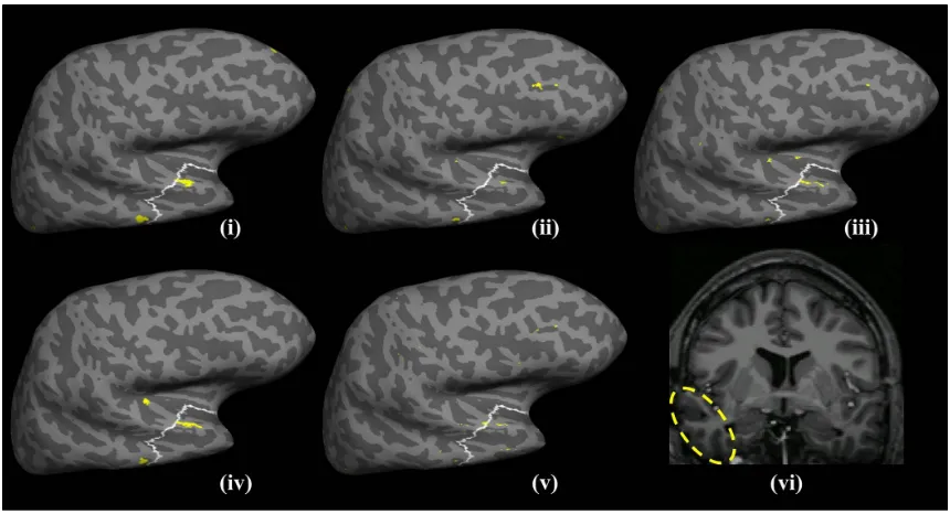
Figure 2: Detection results for NY67 using cortical thickness shown on an inflated model of the lateral cortical surface. The resected region is delineated as the white circled region and the detection results are shown as filled yellow regions. It can be seen that the lesion is detected at individual scales (i) and (iii) prior to combining the outlier probabilities using HCRF. However, at the second scale (ii) a large cluster is detected outside the resection. When these findings are combined using the HCRF as shown in (iv) the largest detected cluser is within the resection zone while the false detection in (ii) is suppressed. (v) shows the detection made by the the z-score based approach. The results are shown for the most stringent (first) threshold without any post-processing. (vi) shows the lesion highlighted on a T1 MRI slice.
the lesional area. This increases the probability that a patch can be entirely formed from lesional vertices, rather than having patches that partially overlap with the lesion, which would be harder to detect as outliers. Based on these settings, the validation set resulted an average of 4255±107 HCRF models per patient, with 19292±373 leaves at the finest scale using cortical thickness. Although the size of the validation set seems small as far as the number of patients are concerned, we conjecture that the resulting number of HCRF models and number of instances are adequate for setting the model parameters.
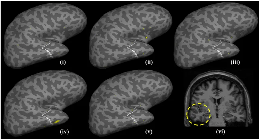
Figure 3: Detection results for NY294 based on curvature. The white outlined area repre-sents the region that was resected, while the filled yellow patches represent the detected clusters at the first detection threshold for both the HCRF and the z-score based method. The detected clusters at the individual scales are shown in (i)-(iii). It can be seen that very small (almost negligible) clusters are detected that overlap with the resected region. However, after running belief propagation (iv) a large cluster is detected within the resection zone while the outliers are eliminated. (v) shows the results for z-score based method while (vi) shows the lesion highlighted on a T1 MRI slice.
4.3 Evaluation Methodology
The final detection for each subject is determined by thresholding the posterior probabil-ities at the leaves of the CRF, which represent the segments obtained at the finest scale. We determine the detection thresholds by dividing the last percentile of the final outlier probabilities into ten equal parts. The first threshold corresponds to the lowest probability in the highest 0.1% scores and so on. For the results presented in this section we determine five such thresholds to get five different possible detections. Because, this is an adaptive mechanism, it has a possible drawback that it always detects something even when the probabilities are very small. Thus we set 1×10⁻⁴ as the minimum probability, such that no threshold is calculated below this value. This limiting value was selected based on the observation that any threshold calculated below this value resulted in more than 80% of the cortex being labeled as lesional for the patients in the validation set.
on the following score function:
score(c;α) =αs(c) + (1−α)o(c) ; 0≤α≤1 (8)
where c is a cluster detected at a pre-defined threshold, s(.) ∈[0,1] is the relative surface area of the cluster calculated as the ratio between the surface area ofcand the total surface area labeled as lesional. o(.) ∈ [0,1] is a scoring function that represents the degree of “outlier-ness” of the cluster. For the HCRF, we model o(.) as the average of the outlier probabilities calculated at each vertex that is part of the cluster. α is a tradeoff parameter such that α = 1 defines a ranking that is based solely on cluster-size, while α = 0 ranks the clusters based only on their average probability of being lesional. Intermediate values of α define a ranking in which a smaller cluster detected at a stringent threshold is ranked higher than a larger cluster detected at a more lenient threshold and vice versa. In the ideal case clusters having a higher rank should be within the lesion/resection zone of the patient. We compare the results of our proposed technique against a recently reported univariate technique (Thesen et al., 2011) to detect FCD lesions using SBM. In this baseline approach all control and subject surfaces are registered to the average surface. After registration, it calculates the z-scores at each vertex for the subjects, which are then thresholded to obtain the detection results. We calculate the z-score based on gender matched controls instead of using all the controls. To facilitate comparison we calculate multiple thresholds in the exact same manner as outlined above for HCRF, and rank the clusters at each threshold based on Equation 8. We omit the last step of the baseline method, which post processes the detections to eliminate “small” clusters (Thesen et al., 2011). We have chosen this technique as the baseline method because, i) it is a semi-supervised approach and does not require accurate vertex-level labels, and ii) it has been part of the pre-surgical evaluation at the NYU comprehensive epilepsy treatment center where the patients included in our evaluation were treated. We use the following measures to evaluate our proposed method.
4.3.1 Detection Rate
Detection rate is defined as the number of patients for whom one or more detected clusters overlap with the resected area. Usually a post-processing step is applied to the raw detec-tions before estimating the detection rate. Hong et al. (2014) train a classifier to distinguish between clusters detected in the resection/lesional area and the extra-lesional clusters using the training data, this classifier is then applied to the clusters detected on the test subject before estimating the detection rate. Similarly, in Thesen et al. (2011) all clusters below a pre-set size threshold are discarded, and a successful detection results if one or more of the remaining cluster overlap with the lesional area. Discarding any detected cluster based on its size increases the risk of discarding subtle lesions. Instead of discarding detected clus-ters, we use cluster ranking to estimate the detection rate. To this end, we calculate five thresholds based on the outlier probabilities for the HRCF method, and similarly for the z-score method. After ranking the detected clusters based on (Equation 8), at each thresh-old we consider a subject to be correctly detected if a cluster amongst the top n (where
4.3.2 Precision and Recall
In order to compare the quality of detections, we calculated the precision and recall for both HCRF and the z-score based method. To this end, we consider all detected clusters at each threshold. We define recall as the ratio of the total surface area of all the clusters that overlap with the resection zone to the surface area of the resection zone. Similarly, we define precision as the ratio of the surface areas of clusters overlapping with the resection zone to the sum of the surface area of all the detected clusters.
Accurately calculating the false postive rate for the proposed detection scheme is chal-lenging for several reasons. A patient can have abnormalities outside the lesion/resection zone which may not be epileptogenic. For example, abnormal cortical thinning remote from the epileptogenic onset region has been observed in focal epilepsy (McDonald et al., 2008; Lin et al., 2007) and attributed to the destructive impact of chronic seizures on brain structure rather than from malformations during cortical development. This might result in elevated extra-lesional false positives when detecting structural malformations charac-terized by abnormal cortical thickness. In our previous work (Ahmed et al. (2014)) we compared our detections on MRI-positive patients with an expert neuroradiologist. In 50% of the cases, the expert identified abnormal regions that coincided with detections outside the resection that were classified as false positives by our evaluation methodology that used the resection zone as the ground truth. This problem becomes more challenging for MRI-negative patients whose structural abnormalities are not visible on their MRI. In order to circumvent the presence of false negatives in our labeled data that would result in elevated estimates of the false positive rate, we use precision to evaluate the efficacy of our proposed scheme. Furthermore, based on the existence of structural abnormalities outside the resec-tion zone (false negatives) the precision estimates provided here should be treated as lower bounds.
4.4 Results
In our experiments we first evaluate the HCRF framework independently for each of the four morphological features: cortical thickness, gray/white-matter contrast, curvature and sulcal depth. In the next set of experiments we analyze different mechanisms of combining the detections from individual features. Recall, that the ranking function (Equation 8) has a direct impact on the detection rate and by setting the tradeoff parameter we can assign more weight to either cluster size or the average cluster outlier probability. To facilitate comparison between the proposed method and the baseline we initially set the tradeoff parameterα to 1, so that all clusters are ranked based only on their surface area.
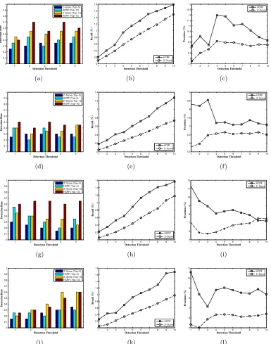
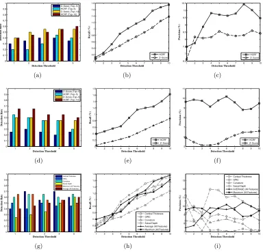
Figure 4(a) shows the comparison of the detection rates for MRI-negative patients when cortical thickness is used to represent the cortex. HCRF performs better than the z-score baseline across all the five thresholds, for the top five detections. HCRF detects the lesion in 14 (70%) patients, while the baseline detects only 11 (55%) subjects when considering the top ten largest clusters. HCRF is also able to achieve higher recall and precision as shown in Figures 4(b)-4(c). The difference between the recall values of the proposed method (1.1140±0.5654) and the baseline (0.8035±0.4745) was significant att(9) = 7.9927, p <
1 2 3 4 5 0 0.1 0.2 0.3 0.4 0.5 0.6 0.7 0.8 0.9 1 Detection Threshold Detection Rate Z−Score (Top−5) HCRF (Top−10) Z−Score (Top−10) HCRF (Top−10) (a)
1 2 3 4 5 6 7 8 9 10
0 0.2 0.4 0.6 0.8 1 1.2 1.4 1.6 1.8 Detection Threshold Recall (%) HCRF Z−Score (b)
1 2 3 4 5 6 7 8 9 10
7.5 8 8.5 9 9.5 10 10.5 11 11.5 12 12.5 13 Detection Threshold Precision (%) HCRF Z−Score (c)
1 2 3 4 5
0 0.1 0.2 0.3 0.4 0.5 0.6 0.7 0.8 0.9 1 Detection Threshold Detection Rate Z−Score (Top−5) HCRF (Top−5) Z−Score (Top−10) HCRF (Top−10) (d)
1 2 3 4 5 6 7 8 9 10
0 0.2 0.4 0.6 0.8 1 1.2 1.4 Detection Threshold Recall (%) HCRF Z−Score (e)
1 2 3 4 5 6 7 8 9 10
5.5 6 6.5 7 7.5 8 8.5 9 Detection Threshold Precision (%) HCRF Z−Score (f)
1 2 3 4 5
0 0.1 0.2 0.3 0.4 0.5 0.6 0.7 0.8 0.9 1 Detection Threshold Detection Rate Z−Score (Top−5) HCRF (Top−5) Z−Score (Top−10) HCRF (Top−10) (g)
1 2 3 4 5 6 7 8 9 10
0 0.2 0.4 0.6 0.8 1 1.2 1.4 1.6 Detection Threshold Recall (%) HCRF Z−Score (h)
1 2 3 4 5 6 7 8 9 10
5 6 7 8 9 10 11 12 Detection Threshold Precision (%) HCRF Z−Score (i)
1 2 3 4 5
0 0.1 0.2 0.3 0.4 0.5 0.6 0.7 0.8 0.9 1 Detection Threshold Detection Rate Z−Score (Top−5) HCRF (Top−5) Z−Score (Top−10) HCRF (Top−10) (j)
1 2 3 4 5 6 7 8 9 10
0 0.2 0.4 0.6 0.8 1 1.2 1.4 1.6 1.8 Detection Threshold Recall (%) HCRF Z−Score (k)
1 2 3 4 5 6 7 8 9 10
5 6 7 8 9 10 11 Detection Threshold Precision (%) HCRF Z−Score (l)
Figure 4: Comparison of detection rates, precision and recall between then HCRF based approach and the baseline method using thickness (a)-(c), GWC (d)-(f), curvature (g)-(i) and sulcal depth (j)-(l). Here, α = 1 so that larger clusters are ranked higher (refer to Equation 8).
Using GWC, HCRF is able to detect abnormal clusters within the resection zones of ten (50%) patients as opposed to the baseline that detects only nine (45%), as shown in Figure 4(d). Figure 4(e) shows the recall for HCRF method (0.6931±0.3702) that is significantly higher (t(9) = 7.1317, p <0.001) than the recall of the baseline method (0.3815±0.2334). Figure 4(f) compares the precision of the HCRF and baseline using GWC. The differences in the precision values for HCRF (7.5286±0.5769) and the baseline (6.4313±0.2987) were found to be significant at t(9) = 4.2350, p= 0.0022 using a paired t-test. Although, using GWC HCRF is able to outperform the baseline, the resulting detection rate is worse than HCRF with cortical thickness.
Figure 4(g) shows the comparison of the detection rates using curvature to represent the cortex. HCRF dominates the z-score baseline across all the five thresholds, for both top five and top ten detections. HCRF detects abnormal clusters within the resection zones of 13 (65%) patients, while the baseline detects only 9 (45%) subjects when the top ten largest clusters are considered. Figures 4(h)-4(i) show that HCRF is able to achieve higher recall and precision, respectively. The difference between the recall values of the proposed method (0.9473±0.4927) and the baseline (0.5549±0.3903) was significant at
t(9) = 8.825, p <0.001. Similarly, the differences in precision for HCRF (8.5373±1.2063) and the baseline (6.6313±0.6597) were found to be significant att(9) = 3.9135, p <0.0035 using a paired t-test. Figure 3 shows the resulting detections from both the HCRF and the baseline when curvature is used to characterize the cortex for an MRI-negative patient.
When sulcal depth is used to represent the cortex, both the HCRF and the baseline method achieve the same detection rate. Both approaches are able to detect abnormal clusters that overlap with the resections of 12 (60%) patients (Figure 4(j)). However, as Figures 4(k)-4(l) show, HCRF is able to achieve higher recall and precision values. The difference between the recall values for HCRF (0.9585±0.5013) and the baseline (0.4891±
0.3165) was significant at t(9) = 7.7730, p <0.001. Similarly, the differences in precision for HCRF (8.7008±0.8541) and the baseline (6.0124±0.4679) were found to be significant att(9) = 8.0983, p <0.001 using a paired t-test.
Using individual features, HCRF is able to achieve a maximum detection rate of 70% while the baseline has a maximum detection rate of 60%, when top ten largest clusters are considered. For the baseline sulcal depth and cortical thickness achieve higher detection rates as compared to GWC and curvature. Cortical thickness outperforms all other features based on its average precision and recall. For the HCRF method sulcal-depth and curvature achieve identical performance with GWC ranking the lowest.
4.5 Combining Features
In this section we explore the question of whether the HCRF based method will achieve a higher detection rate if the detections of the individual features are combined. As a first strategy, we can simply aggregate the posterior probabilities as obtained by the application of HCRF to each individual feature. Because every feature defines its own segmentation of a given parcellation image, it is not possible to directly aggregate the probabilities obtained at the leaves of the HCRF. To solve this issue we map the posterior probabilities obtained at the leaves of the HCRF, back to the cortical surface for each feature and then define a combination rule at every vertex. We use two basic aggregation rules, in the first we average the probabilities across the four features, and in the second each vertex is assigned a probability that is calculated as the maximum of the four individual probabilities. Similarly, for comparison to the baseline method we use the same techniques to calculate a single z-score estimate at each vertex for the baseline.
Aggregation based on averaging is similar to majority vote rule. In this strategy, vertices for whom most of the features have a high probability of being abnormal will be considered abnormal in the final detection. This has the effect of lowering estimation errors leading to a lower false positive rate by smoothing the outlier probabilities at each vertex. The second strategy that uses the maximum across the probabilities would label a vertex as lesional even if one of the features assigns it a higher outlier probability. This would lead to a higher detection rate along with a high number of false positives.
4.5.1 Performance Comparison to Baseline
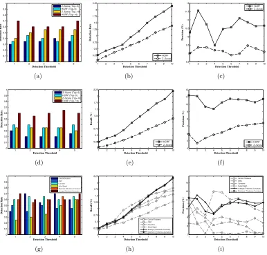
Figure 5 shows the results of applying the two aggregation strategies in conjunction with the HCRF and baseline methods. In particular, Figure-5(a) shows the detection rates when the probabilities are averaged across features. It can be seen that the baseline performs better than the HCRF at the early thresholds, however the HCRF is able to produce better results as the threshold becomes more lenient. Considering the top ten largest clusters, HCRF is able to achieve a detection rate of 60% which is slightly higher than the baseline that achieves a detection rate of 55%. The recall and precision for the HCRF method are significantly higher than the baseline as shown in Figures 5(b)-5(c). Using a paired t-test, the difference in the recall values of the HCRF (1.0206±0.5797) and the baseline (0.7046±0.4410) was significant at t(9) = 7.1317, p < 0.001, and the difference in the precision values of the HCRF (9.2946±0.9708) and the baseline (8.1422±0.5595) was significant at t(9) = 4.2350, p= 0.0022.
When the posterior probability at each vertex is calculated as the maximum across the four features, HCRF achieves higher detection rates as shown in Figure 5(d). HCRF detects abnormal clusters within the resection zones of 13 (65%) patients, while the baseline detects only 10 (50%) subjects when top ten largest clusters are considered. HCRF achieves higher recall (t(9) = 8.825, p < 0.001) and precision (t(9) = 3.9135, p < 0.0035), as shown in Figures 5(e)-5(f), respectively.
4.5.2 Performance Comparison to Individual Features
1 2 3 4 5 0 0.1 0.2 0.3 0.4 0.5 0.6 0.7 0.8 0.9 1 Detection Threshold Detection Rate Z−Score (Top−5) HCRF (Top−5) Z−Score (Top−10) HCRF (Top−10) (a)
1 2 3 4 5 6 7 8 9 10
0 0.2 0.4 0.6 0.8 1 1.2 1.4 1.6 1.8 Detection Threshold Recall (%) HCRF Z−Score (b)
1 2 3 4 5 6 7 8 9 10
6.5 7 7.5 8 8.5 9 9.5 10 10.5 Detection Threshold Precision (%) HCRF Z−Score (c)
1 2 3 4 5
0 0.1 0.2 0.3 0.4 0.5 0.6 0.7 0.8 0.9 1 Detection Threshold Detection Rate Z−Score (Top−5) HCRF (Top−5) Z−Score (Top−5) HCRF (Top−10) (d)
1 2 3 4 5 6 7 8 9 10
0 0.2 0.4 0.6 0.8 1 1.2 1.4 1.6 1.8 Detection Threshold Recall (%) HCRF Z−Score (e)
1 2 3 4 5 6 7 8 9 10
5 6 7 8 9 10 11 Detection Threshold Precision (%) HCRF Z−Score (f)
1 2 3 4 5
0 0.1 0.2 0.3 0.4 0.5 0.6 0.7 0.8 0.9 1 Detection Threshold Detection Rate Cortical Thickness GWC Curvature Sulcal Depth Maximum (All Features) Average (All Features)
(g)
1 2 3 4 5 6 7 8 9 10
0 0.2 0.4 0.6 0.8 1 1.2 1.4 1.6 1.8 Detection Threshold Recall (%) Cortical Thickness GWC Curvature Sulcal Depth Average (All Features) Maximum (All Features)
(h)
1 2 3 4 5 6 7 8 9 10 7 8 9 10 11 12 13 Detection Threshold Precision (%) Cortical Thickness GWC Curvature Sulcal Depth AVERAGE (All Features) Maximum (All Features)
(i)
Figure 5: Comparison of detection rates, precision and recall between then HCRF based approach and the z-score based baseline method when the detection scores are averaged across features (a)-(c), and when the final output score is computed as the maximum across features (d)-(f). (g) contrasts the detection rate of both aggregation strategies with that of the individual features when the top ten largest clusters are considered and (h)-(i) provide the same comparison for recall and precision. Note that α = 1 such that larger clusters are ranked higher (refer to Equation 8).
cortical thickness, and achieve a maximum detection rate of 65% when the top ten largest clusters are considered. The same detection rate is also achieved by curvature. Similarly, based on recall and precision values we can see that both the combination strategies fail to outperform any of the individual features with the exception of GWC.
the other hand, for the averaging technique the differences in recall and precision were not significant when compared to curvature and sulcal depth. For the sake of brevity we omit the results of the paired t-tests that were used to establish these pairwise comparisons.
One reason for the failure of the combined strategies is that each feature has its own idiosyncrasies, which when not accounted for will introduce noise in the ranking/detection process. As an example, consider sulcal depth and curvature. Both features when used within the HCRF framework, achieve similar precision and recall but different detection rates. This shows that although, sulcal depth detects clusters within the resection zones of patients, it detects larger clusters outside the resection zone. If the detections of sulcal depth and curvature are combined then the noisy clusters detected by sulcal depth will cause a drop in the overall detection rate. There are two possible solutions: 1) select only informative features and discard the ones that are noisy, and 2) tune the tradeoff parameter (α) in the ranking function (Equation 8) such that the ranks of smaller clusters that are highly abnormal remain resilient to the presence of larger noisy clusters. It should be noted that changing the ranking function will have no effect on the overall precision and recall, because cluster ranks only influence the detection rate.
To explore option 1, feature selection, we selected cortical thickness and curvature be-cause of their higher detection rates, precision and recall. We employ the same aggregation strategies as before, namely averaging and maximum. In Figure 6 we observe that when using only thickness and curvature, both the averaging and maximum strategies produce higher detection rates, precision and recall than the baseline (Figures 6(a)-6(f)).
More interestingly, when compared to individual features, the combination of curvature and cortical thickness is able to achieve significantly higher precision and recall, with the exception of cortical thickness (the average precision and recall is higher but the differences are not statistically significant), as shown in Figures 6(h)-6(i), respectively. However, as Figure 6(g) shows the detection rate although higher than when all four features are ag-gregated does not exceed that achieved by thickness alone. However these results confirm that when clusters are ranked based only on their size, both GWC and sulcal depth pro-duce noisy detections, that can lower overall detection rate. Our finding that sulcal depth produces noisy or large extra-lesional clusters is also corroborated by Hong et al. (2014).
Next, we explore the effects of tuning the size/probability tradeoff parameter α, on the detection rate of both individual and combined strategies.
4.5.3 Ranking Criterion and the Detection Rate
Thus far we have fixed the ranking criterion to be the size of the detected cluster. However, as defined in Equation 8, we can tune the tradeoff parameter such that the cluster ranking criterion pays attention to both the size and the average outlier probability of the cluster. To ascertain howαinfluences the performance of HCRF framework, we variedαover its entire range of values and determined the detection rate for individual features, the combination of all features, and the combination of the top two features.
1 2 3 4 5 0 0.1 0.2 0.3 0.4 0.5 0.6 0.7 0.8 0.9 1 Detection Threshold Detection Rate Z−Score (Top−5) HCRF (Top−5) Z−Score (Top−10) HCRF (Top−10) (a)
1 2 3 4 5 6 7 8 9 10
0 0.25 0.5 0.75 1 1.25 1.5 1.75 2 2.25 Detection Threshold Detection Rate HCRF Z−Score (b)
1 2 3 4 5 6 7 8 9 10
8.5 9 9.5 10 10.5 11 11.5 12 Detection Threshold Precision (%) HCRF Z−Score (c)
1 2 3 4 5
0 0.1 0.2 0.3 0.4 0.5 0.6 0.7 0.8 0.9 1 Detection Threshold Detection Rate Z−Score (Top−5) HCRF (Top−5) Z−Score (Top−10) HCRF (Top−10) (d)
1 2 3 4 5 6 7 8 9 10
0 0.25 0.5 0.75 1 1.25 1.5 1.75 2 2.25 Detection Threshold Recall (%) HCRF Z−Score (e)
1 2 3 4 5 6 7 8 9 10
4 5 6 7 8 9 10 11 12 Detection Threshold Precision (%) HCRF Z−Score (f)
1 2 3 4 5 0 0.1 0.2 0.3 0.4 0.5 0.6 0.7 0.8 0.9 1 Detection Threshold Detection Rate Cortical Thickness GWC Curvature Sulcal Depth Maximum (Thickness+Curvature) Average (Thickness+Curvature) (g)
1 2 3 4 5 6 7 8 9 10
0 0.25 0.5 0.75 1 1.25 1.5 1.75 2 2.25 Detection Threshold Recall (%) Cortical Thickness GWC Curvature Sulcal Depth Average (Thickness+Curvature) Maximum (Thickness+Curvature) (h)
1 2 3 4 5 6 7 8 9 10
7 8 9 10 11 12 13 Detection Threshold Precision (%) Cortical Thickness GWC Curvature Sulcal Depth Average (Thickness+Curvature) Maximum (Thickness+Curvature) (i)
Figure 6: Comparison of detection rates, precision and recall between then HCRF based approach and the z-score based baseline method when the detection scores are averaged across thickness and curvature (a)-(c), and when the final output score is computed as the maximum between the two features (d)-(f). (g) contrasts the detection rate of both averaging and maximum with that of the individual features when the top ten largest clusters are considered and (h)-(i) compare the recall and precision. Note that, α = 1 so that larger clusters are ranked higher (refer to Equation 8).
0 5 25 50 75 100 0 0.1 0.2 0.3 0.4 0.5 0.6 0.7 0.8 0.9 1
α (%)
Detection Rate Cortical Thickness GWC Curvature Sulcal Depth (a)
0 5 25 50 75 100
0 0.1 0.2 0.3 0.4 0.5 0.6 0.7 0.8 0.9 1
α (%)
Detection Rate
Cortical Thickness Curvature Maximum (All Features) Average (All Features)
(b)
0 5 25 50 75 100 0 0.1 0.2 0.3 0.4 0.5 0.6 0.7 0.8 0.9 1
α (%)
Detection Rate
Cortical Thickness Curvature
Maximum (Thickness + Curvature) Average (Thickness + Curvature)
(c)
Thickness GWC Curvature Sulc Depth Avg. All Max All Avg. Top2 Max Top2 0 0.1 0.2 0.3 0.4 0.5 0.6 0.7 0.8 0.9 1 Detection Threshold Detection Rate Z−Score HCRF (d)
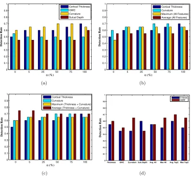
Figure 7: Effect ofα on the detection rates of (a) individual features, (b) combination of all four morphological features and (c) combination of the top two ranked features. In (b) and (c) we have omitted the detection rates of sulcal depth and GWC to improve the clarity of the plot. (d) compares the overall median detection rate of HCRF with the baseline method using different input features and their combinations across the entire range ofα.
Figures 7(b)-7(c) compare the influence of alpha on the detection rates of the two com-bination strategies (averaging and maximum) when all the features are used and when only cortical thickness and curvature are used, respectively. It can be observed that the highest detection rate, 75%, results from using an averaging technique to combine the posterior probabilities of cortical thickness and curvature (Figure 7(c)).
in the case of sulcal-depth, where the baseline is able to outperform HCRF. Similarly, when we combine cortical thickness and curvature to define the final detection, HCRF dominates the baseline, achieving the highest detection rate 75% using an averaging technique to combine the posterior probabilities of the two input features. However, when the same averaging technique is used to combine the results of all four features, both HCRF and the baseline perform comparably (albeit worse than using only two features) and the difference in their performance across the different values of αis not statistically significant.
5. Discussion
Any method of automated detection of FCD lesions is meant to augment the standard comprehensive clinical evaluation protocol for epilepsy surgery candidates. This standard protocol typically involves a neurological exam, scalp electroencephalography (EEG), neu-ropsychological exam, positron emission tomography (PET), and magnetic resonance imag-ing (MRI). Due to the common occurrence of widespread network abnormalities in focal epilepsy, each of these methods has a high rate of false positives. Thus, convergence of evidence from multiple sources is critical to determining the region(s) with the highest like-lihood of hosting the seizure onset zone. In this work, we addressed this challenging task of detecting FCD lesions in a semi-supervised image segmentation framework. To this end, we developed a novel semi-supervised image segmentation method based on hierarchical con-ditional random fields (HCRF). We evaluated the proposed method on four morphological features, and also investigated different mechanisms of combining the outcomes of these input features.
In an empirical evaluation that involved 20 histologically verified MRI-negative pa-tients, who had undergone resective surgery and were subsequently seizure-free, our pro-posed method was able to achieve higher detection rates using four morphological features as compared to a baseline method. Furthermore, when the detections based on these fea-tures were combined, HCRF was still able to detect abnormal clusters within the resection zone of a higher number of patients as compared to the selected baseline. Not only did the proposed method have a high detection rate, it also achieved significantly higher precision and recall across all features and their combinations.
Furthermore, in this work we establish that each of the four morphological features, namely cortical thickness, GWC, curvature and sulcal depth exhibit different behavior for different settings of the cluster ranking criterion and some of them produce noisier detec-tions as compared to others. These two observadetec-tions show that any method that aims at combining the detections from different features should consider feature specific properties such as the false positive rate and adjust the ranking criterion to achieve a high detection rate.
HCRF results have started being incorporated into the weekly meeting of radiologists and neurosurgeons to help identify the seizure onset zones for MRI-negative patients who may be candidates for resective surgery at the New York University´s Comprehensive Epilepsy Center.
As part of the pre-surgical protocol, all patients undergo an intra-cranial EEG (iEEG) exam in which invasive subdural electrodes are placed directly on the cortex to record electrical activity. As a future research direction, we plan to use the results of the iEEG exam to augment the resection zones such that they provide “soft” labels that can be used to jointly learn the parameters of the node and edge potentials in the HCRF. Another avenue of future research is to further expand the feature set to include other features such as diffusivity, connectivity, etc.
Acknowledgments
We thank the reviewers for their helpful comments. We would also like to thank John Brumm, Omar Khan, Hugh Wang and Christine Chao for help with data processing. This research was funded by the Epilepsy Foundation and FACES - Finding A Cure for Epilepsy and Seizures.
References
B. Ahmed, C. E. Brodley, K. E. Blackmon, R. Kuzniecky, G. Barash, C. Carlson, B. T. Quinn, W. Doyle, J. French, O. Devinsky, and T. Thesen. Cortical feature analysis and machine learning improves detection of mri-negative focal cortical dysplasia. Epilepsy & Behavior, 48:21 – 28, 2015.
Bilal Ahmed, Thomas Thesen, Karen Blackmon, Yijun Zhao, Orrin Devinsky, Ruben Kuzniecky, and Carla Brodley. Hierarchical conditional random fields for outlier de-tection: An application to detecting epileptogenic cortical malformations. InProceedings of the 31st International Conference on Machine Learning (ICML-14), pages 1080–1088, 2014.
L.C. Andrews. Special Functions of Mathematics for Engineers. SPIE Optical Engineering Press, 1992. ISBN 9780819426161.
P. Awasthi, A. Gagrani, and B. Ravindran. Image modelling using tree structured condi-tional random fields. InIJCAI, pages 2060–2065, 2007.
M.L. Bell, S. Rao, E.L. So, et al. Epilepsy surgery outcomes in temporal lobe epilepsy with a normal MRI. Epilepsia, 50(9):2053–2060, 2009.
S. R. Benbadis, L. Heriaud, W. O. Tatum IV, and F. L. Vale. Epilepsy surgery, delays and referral patternsare all your epilepsy patients controlled? Seizure, 12(3):167 – 170, 2003.
P. Besson, N. Bernasconi, O. Colliot, et al. Surface-based texture and morphological analysis detects subtle cortical dysplasia. In MICCAI, pages 645–652, 2008.
Christopher M. Bishop. Pattern Recognition and Machine Learning (Information Science and Statistics). Springer-Verlag New York, Inc., 2006. ISBN 0387310738.
I. Blumcke, M. Thom, E. Aronica, et al. The clinicopathologic spectrum of focal cortical dysplasias: A consensus classification proposed by an ad hoc task force of the ILAE diagnostic methods commission. Epilepsia, 52(1):158–174, 2011.
M. Breunig, Hans-Peter Kriegel, R.T. Ng, and J. Sander. LOF: Identifying Density-Based Local Outliers. InACM SIGMOD ICMD, pages 93–104. ACM, 2000.
D. Comaniciu and P. Meer. Mean shift: a robust approach toward feature space analysis. PAMI, 24(5):603–619, 2002.
A.M. Dale, B. Fischl, and M.I. Sereno. Cortical surface-based analysis: I. segmentation and surface reconstruction. NeuroImage, 9(2):179–194, 1999.
R.S. Desikan, F. Sgonne, B. Fischl, et al. An automated labeling system for subdividing the human cerebral cortex on MRI scans into gyral based regions of interest. NeuroImage, 31(3):968–980, 2006.
B. Fischl and A. M. Dale. Measuring the thickness of the human cerebral cortex from magnetic resonance images. Proceedings of the National Academy of Sciences, 97(20): 11050–11055, 2000.
B. Fischl, M.I. Sereno, and A.M. Dale. Cortical surface-based analysis: II: Inflation, flat-tening, and a surface-based coordinate system. NeuroImage, 9(2):195–207, 1999a.
B. Fischl, D.H. Salat, E. Busa, et al. Whole brain segmentation: Automated labeling of neuroanatomical structures in the human brain. Neuron, 33(3):341–355, 2002.
Bruce Fischl, Martin I. Sereno, Roger B.H. Tootell, and Anders M. Dale. High-resolution intersubject averaging and a coordinate system for the cortical surface. Human Brain Mapping, 8(4):272–284, 1999b.
W. A. Hauser and D. C. Hesdorffer.Epilepsy: frequency, causes and consequences. Epilepsy Foundation of America, 1990.
S. J. Hong, H. Kim, D. Schrader, N. Bernasconi, B. C. Bernhardt, and A. Bernasconi. Automated detection of cortical dysplasia type II in MRI-negative epilepsy. Neurology, 83(1):48–55, 2014.
Nathalie Japkowicz and Mohak Shah. Evaluating Learning Algorithms: A Classification Perspective. Cambridge University Press, New York, NY, USA, 2011. ISBN 0521196000, 9780521196000.
Ruben I. Kuzniecky and A.James Barkovich. Malformations of cortical development and epilepsy. Brain and Development, 23(1):2 – 11, 2001.
P. Kwan and M. J. Brodie. Early identification of refractory epilepsy. New England Journal Of Medicine, 342(5):314–319, 2000.
J. T. Lerner et al. Assessment and surgical outcomes for mild type I and severe type II cortical dysplasia: a critical review and the UCLA experience.Epilepsia, 50(6):1310–1335, 2009.
J.J. Lin, N. Salamon, A.D. Lee, et al. Reduced neocortical thickness and complexity mapped in mesial temporal lobe epilepsy with hippocampal sclerosis. Cereb. Cortex, 17(9):2007– 2018, 2007.
D.G. Lowe. Object recognition from local scale-invariant features. In ICCV, pages 1150– 1157, 1999.
C.R. McDonald, D. J. H. Jr, M. E. Ahmadi, et al. Regional neocortical thinning in mesial temporal lobe epilepsy. Epilepsia, 49(5):794–803, 2008.
C.W. Nordahl, D. Dierker, I. Mostafavi, et al. Cortical folding abnormalities in autism revealed by surface-based morphometry. J Neurosci., 27(43):11725–11735, 2007.
S. Papadimitriou, H. Kitagawa, P.B. Gibbons, and C. Faloutsos. LOCI: fast outlier detection using the local correlation integral. In ICDE, pages 315–326, 2003.
J. Pearl. Probabilistic Reasoning in Intelligent Systems: Networks of Plausible Inference. Morgan Kaufmann Publishers Inc., 1988. ISBN 1558604790.
R. Pienaar, B. Fischl, V. Caviness, N. Makris, and P. E. Grant. A methodology for analyzing curvature in the developing brain from preterm to adult.International Journal of Imaging Systems and Technology, 18(1):42–68, 2008.
N. Plath, M. Toussaint, and S. Nakajima. Multi-class image segmentation using conditional random fields and global classification. In ICML, pages 817–824, 2009.
J. Reynolds and K. Murphy. Figure-ground segmentation using a hierarchical conditional random field. In CRV, pages 175–182, 2007.
L.M. Rimol, R. Nesvg, D.J. Hagler Jr., et al. Cortical volume, surface area, and thickness in schizophrenia and bipolar disorder. Biological Psychiatry, 71(6):552–560, 2012.
D. H. Salat, R. L. Buckner, A.Z. Snyder, et al. Thinning of the cerebral cortex in aging. Cerebral Cortex, 14(7):721–730, 2004.
E. Schubert, R. Wojdanowski, A. Zimek, and Hans-Peter Kriegel. On evaluation of outlier rankings and outlier scores. InSDM, pages 1047–1058, 2012.
T. Thesen, B.T. Quinn, C. Carlson, et al. Detection of epileptogenic cortical malformations with surface-based MRI morphometry. PLoS ONE, 6(2):e16430, 2011.
J. F. Tllez-Zenteno, R. Dhar, and S. Wiebe. Long-term seizure outcomes following epilepsy surgery: a systematic review and meta-analysis. Brain, 128(5):1188–1198, 2005.
D. C. Van Essen, H. A. Drury, S. Joshi, and M. I. Miller. Functional and structural mapping of human cerebral cortex: Solutions are in the surfaces. Proceedings of the National Academy of Sciences, 95(3):788–795, 1998.
A. Vedaldi and B. Fulkerson. VLFeat: An open and portable library of computer vision algorithms. http://www.vlfeat.org/, 2008a.
A. Vedaldi and S. Soatto. Quick shift and kernel methods for mode seeking. In ECCV, pages 705–718, 2008b.