Iranian Journal of Electrical and Electronic Engineering, Vol. 15, No. 2, June 2019 222
Design of Fractional Order Sliding Mode Controller for Chaos
Suppression of Atomic Force Microscope System
S. Haghighatnia* and H. Toossian Shandiz**
(C.A.)Abstract: A novel nonlinear fractional order sliding mode controller is proposed to control the chaotic atomic force microscope system in presence of uncertainties and disturbances. In the design of the suggested fractional order controller, conformable fractional order derivative is applied. The stability of the scheme is proved by means of the Lyapunov theory based on conformable fractional order derivative. The simulation results show the advantages of the designed controller such as fast convergence speed, high accuracy and robustness against uncertainties and disturbances.
Keywords: Conformable Fractional Order Derivative, Chaotic System, Atomic Force Microscope System, Fractional Order System, Fractional Order Sliding Mode Controller.
1 Introduction1
HE atomic force microscope is a known device for imaging the topography of surfaces and surface analysis applications with the precise measurements at the nano-scale [1]. The atomic force microscope is composed of a probe with a microscopic tip joined to a cantilever. The force between probe tip and the sample surface leads to cantilever deviation. Using optical methods, cantilever deflection is calculated. Micro-cantilever has chaotic behavior under in the specific conditions [2]. In [3], the micro-cantilever is modelled. Also, in order to suppress the chaotic behavior of atomic force microscope, a proportional and derivative controller is presented. In [4], a robust feedback controller is developed to control the chaotic behavior of atomic force microscope system. In order to control the chaotic behavior of atomic force microscope system, two control schemes are investigated in [5].
Fractional calculus is known as an effective tool in
Iranian Journal of Electrical and Electronic Engineering, 2019. Paper first received 17 February 2018 and accepted 08 September 2018.
* The author is with the Electrical and Robotic Engineering Faculty, Control Department, Shahrood University of Technology, Shahrood, Iran.
** The author is with the Engineering Faculty, Electrical Department, Ferdowsi University of Mashhad, Mashhad, Iran.
E-mails: [email protected] and
Corresponding Author: H. Toossian Shandiz.
many applications. So far, several definitions of fractional order derivatives have been presented [6]. Recently, conformable fractional order derivative as a new definition of fractional order derivative is introduced. One of important its advantages is having simple calculation [7]. Various papers have been presented based on conformable fractional order derivatives. In [8], some important laws and definitions based on conformable fractional order derivative are presented. Fractional Newtonian mechanics based on conformable fractional calculus are studied in [9]. Stability of fractional differential systems is discussed using conformable fractional order derivative in [10]. Sliding mode controller is an effective strategy to control systems with uncertainties and disturbances. In [11], two new nonlinear sliding mode controllers are developed. In [12], a chattering-free full-order nonlinear sliding mode controller is developed. In order to control type I diabetes in presence uncertainties and disturbances, a fractional order sliding mode controller and adaptive fractional order sliding mode controller are designed in [13]. For an uncertain manipulator, a fuzzy robust fractional order controller is developed in [14]. Fractional sliding mode schemes are presented to track and stabilize some nonlinear fractional-order systems with uncertainty in [15].
In this study, a fractional order sliding mode controller involving a novel switching function based on conformable definition is designed to remove chaotic behavior of atomic force microscope system. The stability analysis for the proposed controller is discussed
T
Iranian Journal of Electrical and Electronic Engineering, Vol. 15, No. 2, June 2019 223 using Lyaponuv theorem based on conformable
operators. The simulation results show the effectiveness of the developed controller.
The paper is organized as follows: Some mathematical preliminaries are presented in Section 2. Mathematical model of atomic force microscope system is introduced in Section 3. In Section 4, fractional order Lyapunov stability based on conformable fractional order derivative is investigated. A novel fractional order sliding mode controllers with conformable fractional order derivative is discussed in Section 5. Section 6 demonstrates simulation results of the suggested scheme. Finally, Section 7 concludes this article. 2 Basic Definitions and Preliminaries
In this section, some basic definitions and preliminaries of fractional calculus are presented. Definition 1 [7]. The below fractional order definition is called conformable fractional derivative.
1 0
( ) ( )
( )( ) limf t t f t
T f t
(1)
where f: [0,∞) → R and 0 < α < 1.
Definition 2 [7]. The conformable fractional order integral is defined as:
1 ( ) ( ) t a
a
f t
T f t dt
t
(2)where, α∈ (0, 1).
Theorem 1 [7]. Consider f(t) be a continuous function such that tI0 f t( ) exists. Then,
0
( )( ) ( ), for 0
tT tI f t f t t
(3)
where, α∈ (0, 1].
Definition 3 [8]. The fractional Laplace transform of order α of f (t) is defined as:
0
0
0
1 0
( )
t t s t
t
L f t s e f t t t dt
(4)where, α∈ (0, 1] and f: [t0,∞) → R.
Lemma 1 [8]. Consider f: R+ →R, its fractional
Laplace transform is defined as
0
1 0
t
L f t s L f t t s
(5)
where,
0
{ ( )}( ) st ( )
L g t s
e g t dt .Theorem 2 [7]. Consider α-differentiable functions f(.) and g(.), some properties of conformable fractional order derivatives are as
1) Tα(af+bg)=aTα(f)+bTα(g), for all a, b∈ R 2) Tα(tp)=ptp-α for p∈ R
3) Tα(𝜆)=0, for all constant functions f(t)=λ 4) Tα(fg)=fTα(g)+gTα(f)
5) T ( )f gT ( )f 2fT ( )g
g g
6) If f(.) is differentiable, then T ( )f t1 df ( )t
dt
where α∈ (0, 1].
In this paper, the notations Tα and T-α denote conformable fractional order derivative and integral, respectively.
3 Mathematical Model of Atomic Force Microscope System
The mathematical model of atomic force microscope system in presence of uncertainties and external disturbances is described by:
1 2
2 ( ) ( ) ( )
x x
x f t f d t u t
(6)
where 1 2
1 1 2 3 4 5 2
1
( ) ( cos )
( )
a a
f t a x a a a x
x z
,
|d(t)| ≤ D and |∆f(X)| ≤∆ are external disturbances and system uncertainties, respectively [4].
4 Stability Analysis
In this section, the Lyapunov direct method is investigated by using conformable fractional order derivative.
Consider conformable fractional dynamic system as follows:
0 ( ( )) ( , ( ))
tT x t f t x t
(7) where,f(t, x(t))is a nonlinear function that describes dynamics of the system (7).
Definition 4. The system (7) is conformable stable, if its solution satisfies the below inequality:
0
( ) 0
( ( ))
t t
x h x t e
(8)
where, t0 is the initial time, α ∈ (0,1), λ > 0, b > 0,
h(0) = 0, h(x(t0)) ≥ 0. The inequality (8) is the solution
of Eq. (7) such that its origin is stable.
In the sequel, without loss of generality, we assume that the equilibrium point is in the origin.
Theorem 3. Assume that there exist a Lyapunov function as V(t,x(t)): [0,∞)×D→R. If it satisfies (9) and
(10), the equilibrium point is conformable stable.
1 ( , ( )) 2
a ab
l x V t x t l x (9)
3
( , ( )) ab
t
T V t x t l x (10)
Iranian Journal of Electrical and Electronic Engineering, Vol. 15, No. 2, June 2019 224 where, t ≥ 0, α ≥ 0, α ∈ (0,1), l1, l2, l3, a and b are
arbitrary positive constants.
Proof. By using Ref. [16], according to (9) and (10), we
have 3
2
( , (( )) l ( , ( ))
T V t x t V t x t
l
.
Taking the fractional Laplace transform yields to: 1
3 2
( ) (0) ( )
sV s V l l V s (11)
Thus, we have
3 2 (0) ( ) V
V s l s l (12)
where V(0) = V(0,x(0)) ≥ 0.
Applying inverse fractional Laplace transform to the
(12), 3 0 2 ( ) ( )
( ) (0)
l t t l
V t V e
is obtained. According to
(9) and (10),
3 0 2 ( ) 1 ( ) 1 (0) [ ] l t t l a V x e i
is achieved.
Consider h(t) as follows:
1 1
(0) (0, (0))
( ) V V x 0
h t
l l
(13)
Hence, we have:
3 0 2 ( ) 1 ( ) ( ) [ ] l t t l a
x t he
(14)
So, system (7) is conformable stable. 5 Design Procedure
In this section, the design procedure of new fractional order sliding-mode controller is presented. The design of the proposed fractional order sliding mode controller involves developing nonlinear fractional order sliding surface with desired system dynamics as well as switching function design.
The sliding surface is proposed as
1.5 1.5
1 1 1 2 2 3 1 4 2
2
2 1 1 1 1 2
tanh . . . .
. tanh q
S t
T b c x c x c x c T x
T x m x k T x x
(15)
where α∈ (0, 1) and q∈ (0, 1).
Taking the time derivative of the above equation, one
can obtain:
1.5 1.51 1 1 2 2 3 1 4 2
2
2 1 1 1 1 2
tanh
tanh q
T S t
b c x c x c x c T x
x m x k T x x
(16)
For obtaining equivalent control law, sliding surface derivative must satisfy the below equation.
( ) 0
T S t (17)
In absence of uncertainty and according to system dynamics, the equivalent control is obtained as:
1 1
1.5 1.5
1 1 1 2 2 3 1 4 2
2
1 1 2
( )
tanh( )
tanh
eq
q
u t m x f t
b c x c x c x c T x
k T x x
(18)
Afterwards, the reaching law is designed as:
1 2 3
( ) . tanh . ( ) . ( ) . ( )
r
u t k a s t a T s t a Ts t (19)
Since the control law is u(t) = ueq(t)+ur(t), so using (18)
and (19) yields:
1 1 1.5 1.51 1 1 2 2 3 1 4 2
2
1 1 2
1 2 3
( ) . ( )
tanh . . . .
tanh
. tanh . . .
q
u t m x f t
b c x c x c x c T x
k T x x
k a s a T s a T s
(20)
Theorem 4. The dynamics of the fractional order system under sliding mode controller (20) is asymptotically stable and its state trajectories approach to origin finite time.
Proof. Let us consider the Lyapunov function candidate as:
2 2
2 1 1
1
( ) ( ) . ( )
2
v t x t m x t (21)
The derivative of V(t) is given by
2 2 1 1
2 1 1
1 2
( ) ( ) ( ) ( ) ( )
( ) ( ) . ( ) ( ) ( ) ( )
( ) ( )
v t x t x t x t x t
x t f t m x t f t d t u t
x t x t
(22)
According to (6) and (20), we have (23).
1.5 1.5
2 1 1 1 1 1 2 2 3 1 4 2
2 2
1 1 2 1 2 3 1 1 2 2 2
tanh
tanh q ( ) ( ) tanh
v t x t f t d t m x t b c x t c x t c x t c T x t
k T x t x t k a s t a T s t a T s t m x t x t m x t
(23)
Iranian Journal of Electrical and Electronic Engineering, Vol. 15, No. 2, June 2019 225 Simplifying the above equation, results in
2 1 1
1.5
1 1 1 2 2 3 1
1.5
4 2
2
1 1 2
1 2 3
1 1 2 2 1 1
tanh . .
tanh tanh
] q
v t x f t d t m x t
b c x t c x t c x t
c T x t
k T x t x t
k a s t a T s t a T s t
m x t x t x D b k k
For the below condition, v t( )0 is achieved.
1 1
k k D b (24)
This completes the proof.
Theorem 5. The state trajectories of the controlled system (6) by the controller (20) converge to the nonlinear fractional order sliding surface s = 0 in a finite time.
Proof. Considering V(s) = ½s2(t), one has
SMC
T V t S t T S t
s t (25)Substituting Eq. (16) in Eq. (25) yields,
1 1 1 2 2
1.5 1.5
3 1 4 2
1 1
2
1 1 2
1 1
1.5
1 1 1 2 2 3 1
1 1.5 4 2 1 2 tanh tanh tanh tanh SMC q q
T V S t T S t
S t b c x t c x t
c x t c T x t
f t u t m x t
k T x t x t
S t f t f t d t u t m x t
b c x t c x t c x t
s
ds t dt c T x t
s
T x t x t
(26)
Thus, we have:
1 1 1.5 1.51 1 1 2 2 3 1 4 2
1 2
tanh
tanh ( )
SMC
q
T V t S t T S t
S t f t f t d t u t m x
b c x c x c x c T x
T x x
(27)
From Eq. (20), we have
SMC
T V t S t f t f t d t
1.5 1.51 1 1 1 1 2 2 3 1 4 2
2
1 1 2
1 2 3 1 1
1.5 1.5
1 1 1 2 2 3 1 4 2
1 2
tanh . .
tanh tanh . tanh tanh q q
m x b c x c x c x c T x
f t k T x x
k a s a T s a T s m x
b c x c x c x c T x
T x x
(28)
Simplifying the (29) results in:
1 2 3
1
2 3
tanh
( ) tanh ( )
( ) ( )
( ) SMC
T V t
s t f t d t
k a s t a T s t a T s t
s t D k a s t
a T s t a T s t
s t
(29)
Then:
1 2 3
tanh
D k a s a T s a T s
D k
(30)
So, for |∆|+|D|+η ≤ k, the proof is completed.
The state trajectories of the controlled system will converge to zero asymptotically. In the following, the convergence to zero in finite time is shown.
According to reaching condition Eq. (25):
( ) ( ) ( ) ( )
T V t s t T s t
s t (31)where, T s t( ) t1 ds t( ) dt . So
1 ( )
( ) ( )
s t
ds t t dt
s t
(32)
Integration from both sides of the above equation, we have:
( )
(0) ( ) ( )
0 (0) ( ) 0
0 (0) ( ) 0
r
s t
r s
r
sign s t s t t
s s t
t
s s t
(33)So, the reaching time is as:
(0) r
t s
(34)
Iranian Journal of Electrical and Electronic Engineering, Vol. 15, No. 2, June 2019 226 6 Simulation Results
This section is utilized to confirm the performance of the designed scheme. Consider the atomic force microscope system (6) with the follow parameters [4].
1 4 27
a , a2 1.2, a3 1, a4 2.9, a5 0.1,
2.5
z , f 0.1sin(4x1)sin(4x2) and
( ) 0.2sin(0.5 )
d t t .
Where, the parameters of controller are gained by manipulating as follow:
1 4 27
m , b11.8, c130, c210, c3 30, c4 30,
1 4.5
k , k 0.4,
0.97,
0.65, q0.75. The control input is activated from t = 50. For the initial value [x1(0) x2(0)], T = [0, 0]T.Fig. 1 demonstrates the state trajectories of the controlled system (6) under control law (20). Fig. 2 shows the control input. The simulation results demonstrate the advantages of the proposed method such as fast convergence and high accuracy. Also, it is obvious that using conformable fractional order operators leads to simple mathematic calculations in control design procedure.
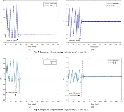
Figs. 3 and 4 show the proposed controller improved the convergence speed compering with [11] and [12]. Fig. 3 represents the results applying the proposed controller in comparison with the designed controller adopted from [11] with the control law as
9 9
23 16
2 2 1
( ) 7 sgn 10 n
u f t x x x u (35)
where 1 2
1 1 2 3 4 5 2
1
( ) ( cos )
( )
a a
f t a x a a a x
x z
and
0.1
n n
u u v , v 10sgn( )s .
Fig. 4 shows the state trajectories of the controlled system in comparing with the controller adopted from [12] with the control law as
1/5
2 2
( ) 2 0.01 s 0.2
u f t g z s
s
(36)
where 1 2
1 1 2 3 4 5 2
1
( ) ( cos )
( )
a a
f t a x a a a x
x z
,
2 1( 1[( 1 1) 2])
g b b b z z and b1 0.2. In Fig. 5, control inputs are illustrated. 7 Conclusion
This article introduces the fractional order sliding mode controller with the novel fractional order switching law to stabilize and suppress the chaotic behaviour of atomic force microscope in presence of uncertainty and disturbance. The control scheme is based on conformable fractional order derivative. The
developed controller has some advantages such as quick convergence speed, high accuracy and robustness against uncertainties and disturbances. The finite-time stability analysis is performed by using the Lyapunov theory based on conformable fractional order derivative. Finally, simulation results are given to show the efficiency of the proposed scheme.
(a)
(b)
Fig. 1 Responses of system state trajectories; a) x1 and b) x2.
Fig. 2 The control law u.
Iranian Journal of Electrical and Electronic Engineering, Vol. 15, No. 2, June 2019 227
(a) (b)
Fig. 3 Responses of system state trajectories; a) x1 and b) x2.
(a) (b)
Fig. 4 Responses of system state trajectories; a) x1 and b) x2.
Fig. 5 Control inputs.
Iranian Journal of Electrical and Electronic Engineering, Vol. 15, No. 2, June 2019 228 References
[1] H. J. Butt, B. Cappella, and M. Kappl, “Force measurements with the atomic force microscope: Technique, interpretation and applications,” Surface Science Reports, Vol. 59, pp. 1–152, 2005.
[2] N. A. Burnham, A. J. Kulik, G. Germaud, and G. A. D. Briggs, “Nanosubharmonics: The dynamics of small nonlinear contacts,” Physical Review Letters, Vol. 74, pp. 5092–5095, 1995.
[3] M. Ashhab, M. V. Salapaka, M. Dahleh, and I. Mezic, “Dynamical analysis and control of microcantilevers,” Automatica, Vol. 35, pp.1663– 1670, 1999.
[4] C. C. Wanga, N. S. Pai, and H. T Yau, “Chaos control in AFM system using sliding mode control by backstepping design,” Communications in Nonlinear Science & Numerical Simulation, Vol. 15, pp. 741–751, 2010.
[5] R. Nozaki, J. M Balthazar, A. M. Tusset, B. R. de Pontes Junior, and Á M Bueno, “Nonlinear control system applied to atomic force microscope including parametric errors,” Journal of Control,
Automation and Electrical Systems, Vol. 24,
pp. 223–231, 2013.
[6] D. Valerio, J. J. Trujillo, M. Rivero, J. A. T. Machado, and D. Baleanu, “Fractional calculus: A survey of useful formulas,” European
Physical Journal Special Topics. Vol. 222,
pp. 1827–1846, 2013.
[7] R. Khalil, M. Al Horani, A. Yousef, and M. Sababheh, “A new definition of fractional derivative,” Journal of Computational and Applied Mathematics, Vol. 264, pp. 65–70, 2014.
[8] T. Abdeljawad, “On conformable fractional calculus,” Journal of Computational and Applied Mathematics, Vol. 279, pp. 57–66, 2015.
[9] W. S. Chung, “Fractional Newton mechanics with conformable fractional derivative,” Journal of
Computational and Applied Mathematics, Vol. 290,
pp. 150–158, 2015.
[10]H. Rezazadeh, H. Aminikhah, and A. H. Refahi Sheikhani, “Stability analysis of conformable fractional systems,” Iranian Journal of Numerical Analysis and Optimization, Vol. 7, No. 1, pp 13–32, 2017.
[11]S. Shoja Majidabad, H. Toosian Shandiz, A. Hajizadehb, and H. Tohidi, “Robust block control of fractional-order systems via nonlinear sliding mode techniques,” Control Engineering and Applied Informatics, Vol. 17, No. 1 pp. 31–40, 2015. [12]Y. Feng, F. Han, and X. Yu, “Chattering free
full-order sliding-mode control,” Automatica, Vol. 50, pp. 1310–1314, 2014.
[13]H. Heydarinejad and H. Delavari, Theory and
Applications of Non-integer Order Systems:
Adaptive Fractional Order Sliding Mode Controller Design for Blood Glucose Regulation-4-3, Springer International Publishing, 2017.
[14]V Kumar, K. P. S. Rana, J Kumar, P Mishra, and S. S. Nair, “A Robust Fractional Order Fuzzy P+Fuzzy I+Fuzzy D Controller for Nonlinear and Uncertain System,” International Journal of
Automation and Computing, Vol. 14, No. 4. pp 474–
488, 2017.
[15]B. Jakovljević, A. Pisano, M. R. Rapaić, and E. Usai, “On the sliding-mode control of fractional-order nonlinear uncertain dynamics. International journal of robust and nonlinear control,” Vol. 26, pp. 782–798, 2016.
[16]Y. Li, Y. Q. Chen, and I. Podlubny, “Mittag-Leffler stability of fractional order nonlinear dynamic systems,” Automatica, Vol. 45, pp. 1965–1969, 2009.
S. Haghighatnia has received the B.Sc.
degree in Electrical Engineering from Sadjad University of Technology, Mashhad, Iran, 2009, the M.Sc. degree in Control Engineering from Islamic Azad University, Mashhad, 2012. She is now a Ph.D. Student in Shahrood University of Technology, Shahrood, Iran. Her fields of research are the optimization, nonlinear control strategies, variable structure control and fractional control.
H. Toossian Shandiz has received B.Sc.
and M.Sc. degree in Electrical Engineering from Ferdowsi Mashad University in Iran. He has graduated Ph.D. in Instrumentation from UMIST, Manchester UK in 2000. He has been Associate Professor in Shahrood University of Technology, Iran. His fields of research are Fractional control, identification systems, adaptive control, Image and signal processing, neural networks and Fuzzy systems.
© 2019 by the authors. Licensee IUST, Tehran, Iran. This article is an open access article distributed under the terms and conditions of the Creative Commons Attribution-NonCommercial 4.0 International (CC BY-NC 4.0) license (https://creativecommons.org/licenses/by-nc/4.0/).
![Fig. 4 shows the state trajectories of the controlled system in comparing with the controller adopted from [12] with the control law as](https://thumb-us.123doks.com/thumbv2/123dok_us/21978.2002380/5.595.314.535.169.545/shows-state-trajectories-controlled-comparing-controller-adopted-control.webp)