Method of Wireless Sensor Network Data Fusion

Method of Wireless Sensor Network Data Fusion

Li-li Ma!!_{", Jiang-ping Liu}

Inner Mongolia Agricultural University, Hohhot, Inner Mongolia, China

liujiangping@imau.edu.cn

Ji-dong Luo

Zte Corp, Hohhot City Office, Inner Mongolia, China

Abstract—In order to better deal with large data information in computer networks, a large data fusion method based on wireless sensor networks is de-signed. Based on the analysis of the structure and learning algorithm of RBF neural networks, a heterogeneous RBF neural network information fusion algo-rithm in wireless sensor networks is presented. The effectiveness of information fusion processing methods is tested by RBF information fusion algorithm. The proposed algorithm is applied to heterogeneous information fusion of cluster heads or sink nodes in wireless sensor networks. The simulation results show the effectiveness of the proposed algorithm. Based on the above finding, it is concluded that the RBF neural network has good real-time performance and small network delay. In addition, this method can reduce the amount of infor-mation transmission and the network conflicts and congestion.

Keywords—Wireless sensor networks, information fusion, RBF neural net-works, big data

1

Introduction

Generally, any single aspect of information is incomplete and inaccurate in the process of information monitoring. Heterogeneous information processing needs to be carried out in a timely manner in order to utilize the information to obtain the exact state of the observation target or the complete real-time evaluation results. As a sim-plification and Simulation of human brain, neural network has powerful parallel pro-cessing ability [8]. In computer networks, the most commonly used are BP neural networks and RBF neural networks, and an improved model based on these two works is also adopted [9]. In theory, both BP neural networks and RBF neural net-works can approximate any nonlinear function with arbitrary precision. However, their approximation performance is different due to their different incentive functions [7].

2

Literature review

Powell proposed a radial basis function (RBF) method for multivariable interpola-tion [10]. Broomhead and Lowe firstly applied RBF to the neural network design, and constituted the radial basis function neural network, that is RBF neural network [11]. Poggio and Girosi have proved that RBF neural network is the best approximation of continuous function, and BP network is not the best choice [12].

The RBF network with local excitation function can overcome the defects of the inherent property brought by BP algorithm that it is easy to get into local minimum. And its convergence is also easier to guarantee than the BP network, so the optimal solution can be obtained. Based on the analysis of the structure and learning algorithm of RBF neural networks, a heterogeneous RBF neural network information fusion algorithm in wireless sensor networks is presented [13]. When it is used in heteroge-neous information fusion of cluster head or sink node in wireless sensor networks, wireless transmission only needs to transfer the fusion results. This reduces the amount of data traffic, network conflicts and congestion [14].

3

Method

3.1 RBF information fusion algorithm for wireless sensor networks

RBF neural network in wireless sensor networks adopts hierarchical information fusion structure. Raw data or processed data collected by each sensor node is trans-mitted to the cluster head node (or sink node) in wireless communication mode. After the information fusion, the result is transmitted to the remote database system via the network and base station.

vector and the output weights are far away from the phase RBF layer close to 0. The effects of these small outputs on the underlying linear layer can be ignored. For any weight that is very close to the input vector, the RBF layer outputs a value close to 1. This value is weighted with the sum of the weights of the second layers as the output of the network, and the output layer is the sum of the weighted outputs of the RBF layer.

MATLAB Neural Network Toolbox provides a lot of toolbox functions for radial basis function neural networks. This has an irreplaceable function for the design, analysis and practical application of RBF neural networks using MATLAB. The input and output structures of the hidden layer neurons in the RBF neural network are shown in figure 1:

Wl

-X

bl

wl

wl

.

.

.

x

x

x

r

Fig. 1. Configuration of RBF nerve cell’s input and output

The input of the i neuron to the hidden layer corresponding to the q input of the

in-put layer is

k

j f

q j ji q

i

(wl

-x

)

bl

k

=

"

!

After the transformation of the Gauss function, the input output of the I neuron in the hidden layer produces an output value of

r

2 2

2

2 (

(k - wl -x bl - wl-x bl

-q

i i

q i i

f

q j ji q

i

e

e

e

r

=

=

"

=

2 2

2 ₀₈₃₂₆

8326 0 C -X Wl . C . -X Wl - q i i q i i q i

e

e

r

=

=

!

(3)

For the output layer, the output is the sum of weights for each hidden layer neuron output. The excitation function uses pure linear function. Corresponding to the input of the input layer Q, the output layer neuron output yq _is:

!

"

=

q

r

w

y

1

2

BF network training is divided into 2 steps. The first step is unsupervised learning to train the weights between the input layer and the hidden layer w1. The second step is to train the weights between the hidden layer and the output layer for supervised learning w2. n the training of RBF networks, the determination of the number of neu-rons in the hidden layer is a key issue. In MATLAB, 0 neuneu-rons are trained, and the output is automatically increased by checking the output error. Each time the loop is used, the maximum error is generated by the network, and the corresponding input vector is used as the weight vector to generate a new hidden layer neuron. The error of the new network is then checked, and the process is repeated until the error re-quirement or the maximum number of hidden neurons is reached.

3.2 Application characteristics of RBF information fusion in sensor network in environmental monitoring

The researchers placed sensor nodes in the monitored area of interest, allowing sensors to form networks autonomously. Each node collects information about tem-perature, humidity, light, etc. Because the sensor nodes have computing power and communication ability, they can do some data processing in the sensor network, espe-cially the information fusion process. This can greatly reduce the amount of data traffic and the forwarding burden of the sensor nodes near the gateway, thereby sav-ing the energy of sensor nodes.

4

Result and discussion

In this paper, MATLAB simulation software is used to simulate the RBF neural network. The simulated training data are selected from the values of the groundwater level, channel flow, air temperature, saturation difference, precipitation and evapora-tion measured in the 24 months of a nearby river test well in a mountain area. The relevant groundwater dynamic records were selected as samples, and the samples contained 24 sets of data. The first 19 sets of data are used as training samples, and the 20-24 sets of data are used as test samples. The number of neurons in the input layer of the RBF network depends on the number of factors affecting the groundwater table. There are five factors according to the problem, so these factors were deter-mined for 5. There is only one quantity of output, that is, the depth of the water level, so the number of neurons in the output layer is set to 1. The NEWRB function in MATLAB is used to train the network and automatically determine the number of hidden layer units required. The excitation function of the hidden layer unit is Radbas, the weighted function is Dist and the input function is NetProd. The excitation tion of the output layer neuron is pure linear function Purelin and the weighted func-tion is DotProd. The input funcfunc-tion is Netsum.

The NEWRB function in MATLAB can be used to create a radial basis function neural network. Its call format is: [Nettr]=newrb(PTGOALSPREADMN

DF)

Among them,

P: it is a RXQ dimensional matrix consisting of Q input vectors;

T: it is a SXQ dimensional matrix consisting of Q group target classification vec-tors;

GOAL: mean square error, default to 0;

SPREAD: it is the extension speed of the radial basis function, and is assumed to be 1;

MN: it is the maximum number of neurons and defaults to Q;

DF: it is the number of neurons added between two displays, and is default to 25; Net: it represents the return value and it is a radial basis network;

Tr: it is a return value that is used for training records.

The larger the extension speed of the radial basis function is, the smoother the SPREAD function is fitted. However, excessive SPREAD means that very large numbers of neurons are required to accommodate fast changes in function. If the SPREAD is too small, it means that many neurons are required to adapt to the slow changes in the function. The network performance is not very good. Therefore, in the network design process, it is necessary to use different SPREAD values to try to de-termine an optimal value. The training algorithm implemented by NEWRB function can adaptively determine the structure of radial basis network and do not need to determine the initial weights of the network artificially, thus reducing the randomness of network training.

satisfies the requirement. Therefore, the network creation process is the training pro-cess, the training process is as follows (among them spread=3.2).

NEWRB,neurons=0,SSE=0.309241 NEWRB,neurons=2,SSE=0.168719 NEWRB,neurons=3,SSE=0.153331 NEWRB,neurons=4,SSE=0.112752 NEWRB,neurons=5,SSE=0.105655 NEWRB,neurons=6,SSE=0.0922185 NEWRB,neurons=7,SSE=0.082831 NEWRB,neurons=8,SSE=0.0633244 NEWRB,neurons=9,SSE=0.050543 NEWRB,neurons=10,SSE=0.0421034 NEWRB,neurons=11,SSE=0.0375743 NEWRB,neurons=12,SSE=0.0333595 NEWRB,neurons=13,SSE=0.0229968 NEWRB,neurons=14,SSE=0.0147105 NEWRB,neurons=15,SSE=0.00385266 NEWRB,neurons=16,SSE=0.00157263 NEWRB,neurons=17,SSE=0.000958959 NEWRB,neurons=18,SSE=0.000104851

Fig. 2. Training of RBF neural network

0 2 4 6 8 10 12 14 16 18

Performence is 0.000104851,Goal is 0,0005

10-4

10-3 10-2

10-1

100

101

Tra

nin

g-B

lu

e G

oa

l-Bla

ck

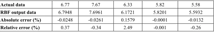
The training result of RBF neural network is shown in figure 2: When the input variables of the network are determined, normalization is needed. In the calculation process, the transformation is set in the range of [-1,1], and the normalized data is easier to train and learn for the neural network. The normalized data is obtained by calculating the deviation between the measured value and the reference value of the corresponding no fault case, and then dividing the absolute value of the maximum deviation to obtain the input variable. The simulated data of the test samples and the RBF neural network are shown in table 1. After the normalization, the comparison of output data and actual data of RBF networks is shown in table 2.

Table 1. Compare of the detection data

Test sample 0.6455 1.0844 0.3816 0.0064 0.1837

RBF output data 0.6178 1.0114 0.3459 0.1922 0.0931

Table 2. Compare of the detection data of the RBF neural network and real data

Actual data 6.77 7.67 6.33 5.82 5.58

RBF output data 6.7948 7.6961 6.1721 5.8201 5.5932

Absolute error (%) -0.0248 -0.0261 0.1579 -0.0001 -0.0132

Relative error (%) 0.37 -0.34 2.49 -0.001 -0.26

When adjusting the Spread value of the NEWRB function in MATLAB, different results can be obtained, and the results are very close to the measured values. From the above simulation results, RBF neural network can predict the data well. After fusing cluster heads or sink nodes in wireless sensor networks, the data concerned can be transmitted directly, such as environmental assessment, environmental tempera-ture, humidity, air quality, and real-time RBF neural network. And the RBF neural network has good real-time performance and small network delay. This feature can save the energy of sensor nodes and prolong the lifetime of the whole sensor network.

5

Conclusion

In the wireless sensor network system of information fusion contract, it is im-portant to study the combination of multiple protocol layers. For example, in applica-tion layer, it is necessary to discuss how to select data gradually through distributed database technology to achieve the effect of fusion. At the network layer, the most important is to study how to introduce the fusion mechanism into the routing protocol to reduce the amount of data transmission.

6

References

[1]Tian, L., & Jing, Z. (2015). A data fusion algorithm based on neural network research in building environment of wireless sensor network. International Journal of Future Genera-tion CommunicaGenera-tion & Networking, 8(78), 2082-7. Https://doi.org/10.14257/jfgcn.2015. 8.4.29.

[2]Bo, L., Hui, Y., Li, T., & Huang, D. (2016). Study on food information online monitoring system utilized wireless sensor network. Advance Journal of Food Science & Technology, 11(2), 137-142. Https://doi.org/10.19026/ajfst.11.2368.

[3]Liu, L., Luo, G., Qin, K., & Zhang, X. (2017). An algorithm based on logistic regression with data fusion in wireless sensor networks. Eurasip Journal on Wireless Communica-tions & Networking, 2017(1), 10. Https://doi.org/10.1186/s13638-016-0793-z.

[4]He, H., Zhu, Z., & Mäkinen, E. (2015). Task-oriented distributed data fusion in autono-mous wireless sensor networks. Soft Computing, 19(8), 1-15. Https://doi.org/10.1007/ s00500-014-1421-7.

[5]G. Santhi, S., & R. Ramya, R. R. (2015). Clustering based data collection using data fusion in wireless sensor networks. International Journal of Computer Applications, 116(9), 21-26. Https://doi.org/10.5120/20364-2569.

[6]Yuan, K., Xiao, F., Fei, L., Kang, B., & Yong, D. (2016). Conflict management based on belief function entropy in sensor fusion:. Springerplus, 5(1), 638. Https://doi.org/10.1186/ s40064-016-2205-6.

[7]Luo, X., & Chang, X. (2015). A novel data fusion scheme using grey model and extreme learning machine in wireless sensor networks. International Journal of Control Automation & Systems, 13(3), 539-546. Https://doi.org/10.1007/s12555-014-0909-8.

[8]Abbassi, M. A. E., Jilbab, A., & Bourouhou, A. (2016). A robust model of multi-sensor data fusion applied in wireless sensor networks for fire detection. , 9(3), 173. Https://doi.org/10.15866/iremos.v9i3.8558.

[9]Yu, J., & Zhang, X. (2015). A cross-layer wireless sensor network energy-efficient com-munication protocol for real-time monitoring of the long-distance electric transmission lines. Journal of Sensors, 2015(5), 1-13. Https://doi.org/10.1155/2015/515247.

[10]Sun, B. (2015). Design and testing of hybrid antenna cluster networking model research based on turntable sink node. Journal of Information & Computational Science, 12(7), 2513-2525. Https://doi.org/10.12733/jics20105306.

[11]Wu, Y. I., Wang, H., & Zheng, X. (2016). Wsn localization using rss in three-dimensional space—a geometric method with closed-form solution. IEEE Sensors Journal, 16(11), 4397-4404.

[13]Sorber, L., Barel, M. V., & Lathauwer, L. D. (2015). Structured data fusion. IEEE Journal of Selected Topics in Signal Processing, 9(4), 586-600. Https://doi.org/10.1109/jstsp. 2015.2400415.

[14]Lahat, D., Adali, T., & Jutten, C. (2015). Multimodal data fusion: an overview of methods, challenges, and prospects. Proceedings of the IEEE, 103(9), 1449-1477. Https://doi.org/10.1109/jproc.2015.2460697.

7

Authors

Li-li Ma (corresponding author) is with the College of Computer and Information Engineering of the Inner Mongolia Agricultural University, Hohhot 010018, Inner Mongolia, China (liujiangping@imau.edu.cn).

Jiang-ping Liu is with the College of Computer and Information Engineering of the Inner Mongolia Agricultural University, Hohhot 010018, Inner Mongolia, China

Ji-dong Luo is with Zte Corp, Hohhot City Office, Hohhot, Inner Mongolia, Chi-na.