An auralisation method for real time subjective testing of modal parameters

AN AURALISATION METHOD FOR REAL TIME SUBJECTIVE TESTING

OF MODAL PARAMETERS

M.Wankling1 And B. Fazenda1

1

University of Huddersfield, Queensgate, Huddersfield HD1 3DH, UK

ABSTRACT

Subjective testing is necessary when attempting to determine the human response to audio quality. Small rooms, such as recording studio control rooms themselves have an effect upon the quality of the perceived audio reproduction. Of particular interest is the low frequency region where resonances, or ‘room modes’, occur. It is necessary to test a number of modal parameters individually and be able to alter them instantly during testing in response to listener perception. An auralisation method has been developed which is used to compare musical samples within modelled rooms. Methods are discussed in the context of providing a practical system, where real time testing is feasible. The formation of the room’s transfer function is discussed, as are a number of issues relating to the generation of audio samples. This work is then placed in context with a brief explanation of how the system is to be used in a real subjective test.

Keywords subjective testing, room modes, auralisation

1 INTRODUCTION

Low frequency audio reproduction within small rooms has long been problematic. In part, problems arise due to room modes - resonances set up as a result of the room's physical boundaries. The problems are prevalent at low frequencies, where the wavelengths are comparable in size to the room dimensions.

Each mode has a specific set of parameters, which combine to form a complex response in both time and frequency domains, unique to each room. Examples of these parameters include frequency distribution, decay time and coupling between sources and receivers. These parameters are in turn affected by factors such as the size and layout of the room, the amount, type and positioning of any absorption present, the placement and design of loudspeakers and the location of the listener.

With so many variables, solutions to modal problems are of great interest to the professional audio industry. Indeed, it can be seen from the literature that a great deal of effort has been placed into the optimisation of small rooms. This optimisation should, in turn, be driven not only by theoretical predictions, but also by informed knowledge of listener perception through subjective testing. Such testing aims to determine threshold levels and listener preferences in order to provide guidelines for those producing optimisation solutions

.

There have been many attempts to produce such solutions, including absorption and diffusion, modal distribution [1-7], loudspeaker positioning [8-10], multiple subwoofers [11] and DSP approaches [12]. There is however, a problem. Each of these methods relies upon theoretical studies in producing objective measures by which to inform those optimising current (or indeed designing new) listening rooms. However, many of them, although some allude to it, do not incorporate subjective psychoacoustic results in their guidelines. In response, some initial work has been carried out, such as investigations into the thresholds of perception of resonance [13,14], and the doctoral thesis of Fazenda [15]. Further work is, however, necessary.

2 VIRTUAL ROOMS

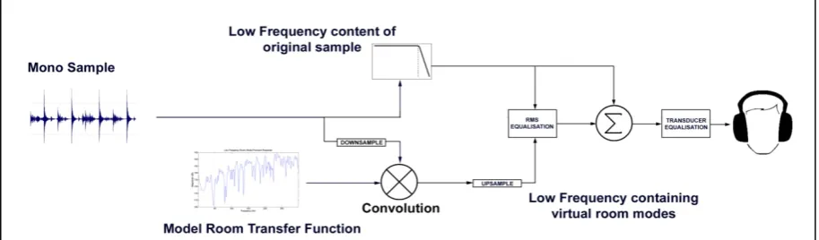
Figure 1 shows the steps necessary to facilitate the testing of modal parameters. The output is a musical sample which can be auditioned over headphones. It is necessary to create virtual listening rooms for three main reasons:

Firstly, the testing procedures commonly require the auditioning of many different spaces. Physical facilities to accommodate this are not available; Secondly, even if suitable facilities existed, the human auditory memory is short [16,17], the result being that transfer of the subject between listening environments would violate their ability to produce an informed comparison; Thirdly, by creating artificial computer simulations, we are able to isolate individual parameters which would otherwise be impossible in real rooms.

With these reasons in mind, we can see that modelling the room is of great benefit. If we can predict the behaviour, we can then reproduce the experience of listening within that room over headphones. As shown in Figure 1, there are a two stages in doing so, firstly, forming a room model, and secondly, producing an auralisation.

2.1 Forming a Room Model

Just as all systems can be characterized by a transfer function, so too can the effect of a room. This transfer function can be predicted from acoustical principles by a room model in either the frequency or time domain.

When forming a room model, we must decide the frequency range in which we are working. As previously stated, within small rooms, it is only in the lower frequency region that problems occur as a result of modal behaviour. Although there are of course issues to contend with in the higher frequency region, these are not within the scope of this research.

It is widely believed that above a certain transition frequency, the sound field may be termed 'diffuse' (see [18] for more information). While the frequency at which this transition occurs is by no means certain [19], it is generally accepted that the Schroeder Frequency [1] provides a good initial guideline. In a typically damped room of 100m3, this would occur at approximately 150-180Hz. This frequency is low enough to enable the prediction of a room by a number of methods. Naturally, both the highest frequency required and the frequency resolution affect the time required to process the impulse response.

A number of methods available to produce the model are briefly discussed.

• Analytical Model. This method is based upon the theoretical work published by Morse [20], and uses a Greens function to calculate the complex pressure output at a particular point in space. Both position of source and receiver are considered, along with damping present. Although there are a number of limitations associated with this method, such as the requirement of a rectangular shape, the assumption of rigid boundaries and its inability to predict high damping cases accurately, advantages are observed in terms of simplicity and speed.

• Image-Source Method. This method also assumes a rectangular room, and is based upon the technique of using sound source images to predict acoustical behaviour. Both the theory and implementation are discussed in detail by Allen and Berkeley [21]. The method has also been used successfully in the search for modal optimization by Cox et al. [2].

The analytical model chosen is represented by the equation:

(Equation 1)

where ρ is the density of the medium, c the velocity of sound, Q the source strength, and Pn(r) and Pn(r0) the

source and shape functions respectively.

This method, known as modal decomposition, has been shown to predict the pressure response at a given point with reasonable accuracy. As Walker points out, the 'overall characteristic of the response were predicted' [18]. He also points out that due to the dependence on the precise position of the source and receiver, real room measurements are difficult to carry out at the exact positions of those chosen in the computer model. Both Avis et al. [19] and Cox et al [4] also provide comparisons between measured responses and those predicted by modal decomposition. Again, both show that the general characteristic is preserved even if the exact frequencies and amplitudes differ slightly.

The model used here is generated within the Matlab software, with additional C programming for speed improvements. A sampling frequency of 2000Hz is used, with the highest frequency available according to the Nyquist theory 1000Hz. 8193 points are generated giving a linear frequency interval of 0.122Hz. Modes are generated only up to 300Hz. The higher sampling frequency eliminates the potential effects of aliasing when transforming to the time domain. The Matlab scripts allow simple adjustment of the x, y and z dimensions as well as source/receiver coordinates and damping within the room.

2.2. Auralisation

The complex pressure response output from Equation 1 must then be transformed into the time domain by IFFT. Prior to this, the pressure output must be translated to a form expected by the IFFT - that is, containing a complex conjugate mirror image. (Fig. 2)

It is important to notice here that there is a transmission period between source and receiver, inherent within the output of the equation. In small rooms, the distance between source and receiver may only be a few meters and yet the resulting time delay is in the order of milliseconds (10 milliseconds for a separation of 3.4m). This difference, if unaccounted for, causes an audible delay of the signal when compared to high frequency regions of the spectrum.

The schematic in Figure 3 explains the basic processing involved in creating a final auralisation sample. A number of papers detail this method [19,22,23], and yet some changes are proposed here and certain aspects discussed in further detail.

There are some interesting factors which must be addressed in order to create a successful sample:

• Choice of high frequency audio

When testing for low frequency artefacts using auralised samples, it is desirable to keep the high frequency components constant. It is widely considered that effects such as reverberation and high frequency masking affect perception at lower frequencies. In previously mentioned work, the high frequency components have consisted of the original music stimulus, convolved with a real impulse response recorded in a typical control room [22,23]. However, the omission of this stage is proposed here. Instead, the original recording’s high frequency content is used. This change is suggested for a number of reasons:

A further consideration is that the measured impulse may not match that of the model. Previous work proposed that using the real rooms high frequency may enhance to impression that we are in a real room. However, these real room characteristics may cause distraction from the low frequency region under study. It remains an interesting investigation as to whether a listener’s result differs when rating samples for their low frequency content with and without realistic high frequency.

Furthermore, if the modelled room is large in volume, a further mismatch would occur as the real impulse is recorded in a small room. The proposed removal of this recorded impulse should allow the listener to better focus their attention on the changing low frequency.

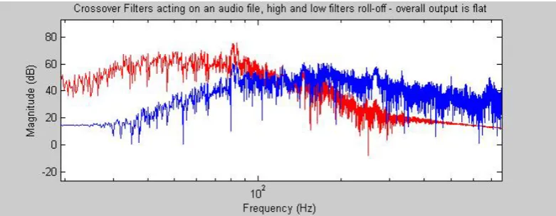
• High/Low crossover

As noted, the crossover filter is an import consideration. The ideal crossover would provide steep attenuation on both sides, with a flat overall response. In some applications, the roll off is particularly important (for example, in loudspeaker design). However, in this auralisation application, the overall flat response is of particular importance. A large addition or reduction in gain at specific frequencies may manifest as an audible colouration, which in the worst cases could lead to incorrect assessments.

The filters have therefore been implemented using Matlab's filtfilt function. This performs zero phase filtering by applying the filter both forwards and then in reverse. This is useful in the processing of audio as there is no phase shift present, and furthermore, the two passes provide double the filter order, allowing not only a steeper roll-off, but also, the paired high and low pass filters imitate the Linkwitz-Riley crossover configuration, providing a flat overall response (Fig. 4)

• Alignment of high and low regions

An important consideration is the alignment of the high and low frequency components. Following the convolution of the low frequency impulse response, a simple addition with the high pass filtered music file results in a mismatch of levels. Furthermore, differing room parameters result in a range of output amplitudes from the room model. In testing, it is required that the bass levels are kept consistent, to ensure that subjects are assessing the quality and are not distracted by level changes. In order to achieve this, a simple matching of RMS levels is performed. The original signal is low pass filtered, and a simple RMS level is determined over the first five seconds. The newly modelled low frequency audio can then be normalized to this value.

• Transducer equalization

Figure 3 shows the final stage as transducer equalization. The headphones used to replay the signals should be equalized to ensure a flat response at low frequencies. Currently, a pair of Sennheiser HD650s are being used. The headphones frequency response is measured by the WinMLS software, and the equalizer comprises a 3000 tap FIR filter, from 20 - 2000Hz. It may be noted that the PC soundcard is also part of the reproduction chain. This is an M-Audio firewire device and is considered an insignificant source of replay error – when taking loopback measurements the device was shown to display a flat response.

3 IN PRACTISE

The following briefly details this method in practice. One modal factor suggested as of particular importance subjectively is the modal decay. This is expected to depend, amongst other things on frequency. The work of Avis et al [22] defines thresholds of modal Q, with an absolute threshold of 16. It is then implied that these Q factors can be extrapolated to decay times. However, no frequency dependence can be inferred from these results, and the Q factor remained fixed, which results in a changing decay threshold. Goldberg has also published work detailing experiments set up to test the threshold of decays. This work however, relates only to artificial signals [24]. Furthermore, Karjalainen et al also investigated modal decay thresholds, this time with music signals [25]. However, the samples were presented in a real room over a loudspeaker, with a single mode added to the response. It is seen here that the auralisation method presented enables both testing of music signals with full room simulations.

would have to be created with a defined minimum interval. It is now possible to fine tune thresholds and reduce possible error.

Here, each time the slider is moved, the scripts are called which firstly create the room model using the newly selected decay time parameter to control damping. The resulting impulse response is then processes as discussed (Fig 3) and the audio output loaded onto the ‘Play Adjustable Sample’ button. For a typical sized room of 100m3, this process requires about 1 second, which is short enough so as not to give the GUI a sluggish feel.

4 CONCLUSION

The auralisation method developed for subjective testing has been presented. A number of points regarding the production of audio samples for low frequency testing have been raised and discussed, with some adjustments suggested from previously used processes.

- The crossover filters between high and low frequency regions provide increased steepness and a flat overall response.

- The proposed high frequency audio should consist of the high pass filtered original music

- The weighting of the modelled low frequency audio should be achieved by taking the average power of the low frequency content in the original sample.

An ongoing subjective test has been introduced, and results are expected to reveal useable thresholds of decay, an important modal parameter, in the context of real signals and real room effects. These results are important to those wishing to optimize or design better listening facilities.

REFERENCES

[1] M.R. Schroeder, “The ``Schroeder Frequency'' Revisited,” J. Acoust. Soc. Am., vol. 99, May. 1996, pp. 3240-3241.

[2] T.J. Cox, P. D'Antonio, and M.R. Avis, “Room Sizing and Optimization at Low Frequencies,” J. Audio

Eng. Soc, vol. 52, Jun. 2004, pp. 640-651.

[3] R.H. Bolt, “Normal Frequency Spacing Statistics,” J. Acoust. Soc. Am., vol. 19, Jan. 1947, pp. 79-90.

[4] M.M. Louden, “Dimension-Ratios of Rectangular Rooms with Good Distribution of Eigentones,”

Acustica, vol. 24, 1971, pp. 101-04.

[5] R. Walker, “Optimum Dimension Ratios for Small Rooms,” Proc. of the 100th AES Convention, 1996. [6] O.J. Bonello, “A New Criterion for the Distribution of Normal Room Modes,” J. Audio Eng. Soc, vol. 19, 1981, pp. 597-606.

[7] C.L.S. Gilford, “The Acoustic Design of Talks Studios And Listening Rooms,” J. Audio Eng. Soc, vol. 27, 1979, pp. 17-3.

[8] A.O. Santillán, “Spatially extended sound equalization in rectangular rooms,” J. Acoust. Soc. Am., vol. 110, 2001, p. 1989.

[9] J.A. Pedersen, “Adjusting a loudspeaker to its acoustic environment: the ABC system,” Proc. of the 115th AES Convention, 2003.

[10] F. Everest, The Master Handbook of Acoustics, New York ;London: McGraw-Hill, 2001.

[11] T. Welti and A. Devantier, “Low-Frequency Optimization Using Multiple Subwoofers,” J. Audio Eng.

Soc, vol. 54, 2006, p. 347.

[12] A. Mäkivirta, P. Antsalo, M. Karjalainen, and V. Välimäki, “Modal equalization of loudspeaker-room responses at low frequencies,” J. Audio Eng. Soc, vol. 51, 2003, pp. 324–343.

[13] S.E. Olive, P.L. Schuck, J.G. Ryan, S.L. Sally, and M.E. Bonneville, “The Detection Thresholds of Resonances at Low Frequencies,” J. Audio Eng. Soc, vol. 45, 1997, pp. 116–127.

[14] R. Bucklein, “The Audibility of Frequency Response Irregularities,” J. Audio Eng. Soc, vol. 29, 1981, pp. 126-131.

[15] B.M. Fazenda, “The Perception of Room Modes,” Doctoral Thesis, University of Salford, UK, 2004. [16] R. Conrad, “Acoustic Confusions in Immediate Memory,” British Journal of Psychology, vol. 55, 1964, pp. 79-80.

[17] R. Crowder and J. Morton, “Precatorgorical acoustic storage,” Perception and Psychophysics, vol. 5, 1969, p. 367.

[19] B.M. Fazenda and M.R. Wankling, “Optimal Modal Spacing and Density for Critical Listening,” Proc.

of the 125th AES Convention, San Francisco: 2005.

[20] P.M.C. Morse, Vibration and sound, McGraw-Hill New York, 1948.

[21] J.B. Allen and D.A. Berkley, “Image method for efficiently simulating small-room acoustics,” J.

Acoust. Soc. Am, vol. 65, 1979, pp. 943–950.

[22] M. Avis, B.M. Fazenda, and W.J. Davies, “Thresholds of detection for changes to the Q factor of low-frequency modes in listening environments,” J. Audio Eng. Soc, vol. 55, Aug. 2007, pp. 611-622.

[23] B. Fazenda, M.R. Avis, and W.J. Davies, “Perception of Modal Distribution Metrics in Critical Listening Spaces-Dependence on Room Aspect Ratios,” J. Audio Eng. Soc, vol. 53, Dec. 2005, pp. 1128-1141.

[24] A. Goldberg, “A Listening Test System For Measuring The Threshold Of Audibility Of Temporal Decays,” Proc. Inst. Acoust., vol. 27, 2005.

[25] M. Karjalainen, P. Antsalo, A. Makivirta, and V. Valimaki, “Perception of Temporal Decay of Low-frequency Room Modes,” Proc. of the 116th AES Convention, Berlin: 2004.

Fig 1 – Flow diagram showing the path which the testing of subjective modal parameters should take

1 2 3 4 … 4096 4097 4098 … 8190 8191 8192

0.1 0.3 0.9 0.8 1.3 2.2 1.3 0.8 0.9 0.3

(no mirror)

(no mirror)

Fig 2 – Flow Mirroring of Pressure Response before IIFT function can be applied, assuming FFT length of 8192 samples

Figure 4: Crossover Filters at 125Hz (red - low pass, blue – high pass)