An Effective Perturbation Iteration Algorithm for Solving Riccati Differential Equations

(1)

An Effective Perturbation Iteration Algorithm for

Solving Riccati Differential Equations

M. Khalid

Department of Mathematical Sciences

Federal Urdu University of Arts, Sciences & Techonology University Road, Karachi-75300, Pakistan

Mariam Sultana

Department of Mathematical Sciences Federal Urdu University of Arts, Sciences & Technology

University Road, Karachi-75300, Pakistan

Faheem Zaidi

Uroosa Arshad

ABSTRACT

In the following study, a novel approach called the Perturbation Iteration Algorithm P IA has been proposed and subsequently adopted for deriving and solving the Riccati differential equation. This new Perturbation Iteration Method is efficient and has no re-quirement of a small parameter assumption as its earlier classical counterparts do. Some examples have been presented to exhibit how simply and efficiently the proposed method works. After de-riving the exact solution of the Riccati equation, the capability and the simplicity of the proposed technique is clarified. A percentage error for each example has also been presented.

Keywords:

Perturbation Iteration Algorithm, Riccati Differential Equation, Analytical Approximation, Convergence

1. INTRODUCTION

The Riccati Differential Equations(RDEs)of the following form:

u0(x) =A(x) +B(x)u(x) +C(x)u2₍_x₎ _x

◦≤x≤X (1) WhereA(x),B(x)andC(x)are given functions andu(x◦) =c, wherecis an arbitrary constant. These are a collection of nonlinear differential equations of immense importance, and have a major role to play in various fields of applied sciences [1]. As an example, take the solitary wave solutions of a nonlinear partial differential equation; it can be represented as a polynomial in two basic functions that maintain the criteria of a projective Riccati equation [2]. Problems such as these also crop up in optimal control literature. In spite of that, deriving an analytical solution in a form that is explicit appears unachievable except in very particular situations [3]. Certainly, if the persons concerned have apt knowledge with respect to a particular solution, the derivation of a general solution is fairly easy. For most cases, one must make use of numerical techniques or approximate approaches for the obtainment of solutions. This is why the problem has

attracted quite a bit of attention in the recent past and has been the topic of study of many authors [4, 5, 6] and the references cited therein. Attaining analytical derivations for the Riccati equation in an explicit form seems an unlikely concept except for certain special situations as discussed above, however, that can easily be overcome if its one particular solution is known. One has to, then, adopt numerical techniques or approximate approaches for getting its solution. In [6], El-Tawil’s study Adomian’s Decomposition Method has been put forward for solving the Riccati differential equations. Abbasbandy solved the equation making use of He’s

V IM, Homotopy Perturbation Method and iterating it. He then matched the accuracy of the obtained solution with the result derived through the Adomian Decomposition Method [5, 7, 8]. On top of that, the Homotopy Analysis Method and a piecewise Variational Iteration Method are introduced for the solution of Riccati differential equations [4, 9]. The Taylor, Chebyshev and Legendre (matrix and collocation) methods have been employed by Sezer et al.[10], and Akyuz [11] to solve the famous Riccati equations.

Every listed method has its own limitations and set-backs in its application. For example, the Adomian Decomposition Method and Variation Iteration Method are limited in that the former involves the usage of complicated algorithms in calculating Adomian polynomials for nonlinear problems, and the latter is inherently inaccuracy when it comes to identifying the Lagrange multiplier which is a necessary factor for the construction of a Variational Iteration formula. The Homotopy Perturbation Method requires solving a linear functional equation in each iteration, and this at times proves to be immensely tricky; sometimes even near impossible. The efficiency of Homotopy Analysis Method depends heavily on choosing auxiliary parameter.

(2)

such as the method of averaging, the renormalization method, the method of multiple scales, the Lindstedt-Poincare method, the method of matched asymptotic expansions, plus their variants were developed to make our results as accurate as possible [12, 13].

The main drawback of perturbation methods is the prerequi-site of a small parameter, which is hard to fulfill. That is why sometimes a small parameter may have to be artificially introduced into the equation. The solutions therefore are not entirely valid. They may be for weakly nonlinear problems, but the validity mostly does not cover strongly nonlinear problems.

Numerous methods have been introduced by researchers in their recent literature to attain admissible solutions which eschew the requirement of a small parameter. Lately, a class of alternative perturbation-iteration algorithms has been proposed, the funda-mentals of which were outlined for the first-order differential equations by Pakdemirli et al.[14]. Multiple iteration algorithms can be equated by taking various number of terms in the pertur-bation expansions and different order of correction terms in the Taylor series expansions. The perturbation iteration algorithm is represented byP IA(n, m) wheren embodies the correction terms in the perturbation expansion andm is the highest order derivative term in the Taylor series. One of the best advantages of the new method is that it does not require initial transformation of the equations to another form. In fact, the technique was first developed for algebraic equations and then tweaked to adapt to ordinary differential equations [14, 15, 16].

In this paper, the iteration algorithm is aptly and tactfully employed to obtain the approximate solution of some nonlinear Riccati differential equations. The competence and accuracy of the method presented is demonstrated with the help of three examples, inclusive of the quadratic Riccati Equation. As it will eventually be proved, the interface of this method is simple and its results fairly accurate Here on wards, the introduction of the Perturbation Iteration Algorithm is presented. In section 3, this algorithm is applied to the Riccati differential equation to solve it with great precision. Conclusive remarks close the paper in Section 4.

2. METHODOLOGY

In this section, a perturbation iteration algorithm is developed by taking one correction term in the perturbation expansion and cor-rection terms of only first derivatives in the Taylor Series expan-sion, i.e.n= 1,m= 1. The algorithm is calledP IA(1,1). Con-sider the general first order differential equation

G(u,u, ˙ ) = 0 (2) withu=u(x)andthe perturbation parameter. Only one correc-tion term is taken in the perturbacorrec-tion expansion

u1=u◦+uc+... (3)

Upon substitution of Eq. 3 into Eq. 2 and expanding in a Taylor series with first derivatives only yields

G(u◦,u˙◦,0) +Gu(u◦,u˙◦,0)uc+

Gu˙(u◦,u˙◦,0)u˙c+G(u◦,u˙◦,0)= 0

(4)

where subscripts denote differentiation with respect to the variable. Reorganizing the equation

˙

uc+

Gu

Gu˙

uc=

G+G

Gu˙

(5)

All derivatives are evaluated at = 0. it is readily observed that the above equation is a variable coefficient first order differential equation whose solution is

uc=c exp

h

−

Z Gu

Gu˙

dti−h

Z _G

+G

Gu˙

exph Z

Gu

Gu˙

dtidti×

exph Z

Gu

Gu˙

dti

(6) Substitution of Eq. 6 into 3 and constructing the iteration scheme yields

un+1=un+cnuc (7)

In this paper, we only consider a casen=m= 1for the sake of simplicity as more Algebra is involved in constructing iteration so-lutions forP IA(1,2)andP IA(1,3)as compared toP IA(1,1). The percentage error, which we will calculate in next section, is de-fined as

%Error=

Exact Solution−N umerical Solution

Exact Solution

×100

(8)

3. ILLUSTRATIVE EXAMPLES

In this work, we use the Perturbation Iteration Algorithm to obtain the approximate solution of some nonlinear Riccati differential equations. Effectiveness and precision of the presented method is shown by three examples.

3.1 Example: 1

Consider the following Riccati equation

u0(x) = 1 + 2u(x)−u2(x) (9) with initial conditionu(0) = 0. For the above differential equation, the exact solution is previously known to be

u(x) = 1 +√2tanh h√

2x+1 2log

√

2−1

√

2 + 1

i

(10)

When we apply Perturbation Iteration Algorithm , Eq. 5 implies

˙

uc=−u˙+ 1

+ 2u−u

2

(11)

Selectingu◦= 0, which satisfies initial condition and using the al-gorithm of perturbation Iteration method, the approximate solution at each step are

u11=x (12)

u12=x+x2−

1 3x

(3)

[image:3.595.75.267.75.231.2]

0 0.2 0.4 0.6 0.8 1 0 0.2 0.4 0.6 0.8 1 1.2 1.4 1.6 1.8 x u(x) Exact u₁₁ u₁₂ u₁₃ u₁₄

Fig. 1. Comparison of solution obtained byP IA(1,1)with exact solution

[image:3.595.321.556.274.587.2]

of Example 1

Table 1. Percentage Error Estimation of Example 1

%Error in %Error in %Error in %Error in

x u11 u12 u13 u14

0.10 9.33422050 9.66666670 0.54660440 0.02539510

0.20 17.34744810 18.66666670 1.79167470 0.15083750

0.30 24.07078750 27.00000000 3.28491560 0.36640910

0.40 29.55416880 34.66666670 4.70540310 0.60012770

0.50 33.86369300 41.66666670 5.81582630 0.76422920

0.60 37.07830780 48.00000000 6.43644790 0.78643160

0.70 39.28612450 53.66666670 6.42952280 0.63129470

0.80 40.58068960 58.66666670 5.68957180 0.31582940

0.90 41.05748040 63.00000000 4.13708150 0.07759120

1.00 40.81083440 66.66666670 1.71428570 0.38854650

%

Mean 31.29837550 42.16666670 4.05513340 0.41066920

Error

u13=x+x2+

1 3x

3₋2

3x

4₋ 1

15x

5

+1 9x

6₋ 1

63x

7

(14)

u14=x+x2+

1 3x

3₋1

3x

4₋3

5x

5₊ 4

45x

6₊ 71

315x

7₊

17 420x

8₋ 62

945x

9₋ 62

4725x

10₊ 27

1925x

11₋ 1

1890x

12₋

41 36855x

13₊ 1

3969x

14₋ 1

59535x

15

(15)

Figure 1 shows comparison between exact solution and iterative solutions of Example 1.It is clear that accurate value is attained as number of iteration increases. Table 1 illustrate percentage errors of each successive solution of Riccati differential equation by per-turbation iteration algorithm.

3.2 Example: 2

u0(x) = 1 +x2−u2(x) (16) with initial conditionu(0) = 1. For the above differential equation, the exact solution is previously known to be

u(x) =x+ e

−x2

1 +Rx

0 e−t

2

dt (17)

When we apply Perturbation Iteration Algorithm , Eq. 5 implies

˙

uc₌ −u˙+ 1 +x

2

−u

2 ₍₁₈₎

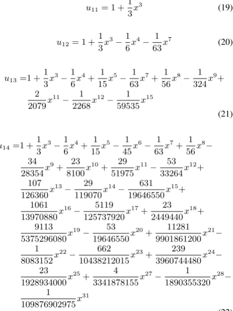
Selecting u◦ = 1 and using algorithm of perturbation Iteration Method, the successive solution are

u11= 1 +

1 3x

3 ₍₁₉₎

u12= 1 +

1 3x

3₋1

6x

4₋ 1

63x

7 ₍₂₀₎

u13=1 +

1 3x

3₋1

6x

4

+ 1 15x

5₋ 1

63x

7

+ 1 56x

8₋ 1

324x

9

+

2 2079x

11₋ 1

2268x

12₋ 1

59535x

15

(21)

u14=1 +

1 3x

3₋ 1

6x

4₊ 1

15x

5₋ 1

45x

6₋ 1

63x

7₊ 1

56x

8₋

34 28354x

9₊ 23

8100x

10₊ 29

51975x

11₋ 53

33264x

12₊

107 126360x

13₋ 29

119070x

14₋ 631

19646550x

15₊

1061 13970880x

16₋ 5119

125737920x

17₊ 23

2449440x

18₊

9113 5375296080x

19₋ 53

19646550x

20₊ 11281

9901861200x

21₋

1 8083152x

22₋ 662

10438212015x

23₊ 239

3960744480x

24₋

23 1928934000x

25₊ 4

3341878155x

27₋ 1

[image:3.595.58.296.280.618.2]

1890355320x 28₋ 1 109876902975x 31 (22)

Figure 2 be evidence for difference between exact and approximate solution obtained

3.3 Example: 3

u0(x) = 1 +u2₍_x₎

[image:3.595.58.293.295.463.2]

(4)

0 0.2 0.4 0.6 0.8 1 0.9

0.95 1 1.05 1.1 1.15 1.2 1.25 1.3 1.35 1.4

x

u(x)

[image:4.595.338.530.74.232.2]

Exact u₁₁ u₁₂ u₁₃ u₁₄

Fig. 2. Comparison of solution obtained by with exact solution of

[image:4.595.71.267.75.231.2]

Exam-ple 2

Table 2. Percentage error of Example 2 withP IA(1,1)

x u11 u12 u13 u14

0.10 0.0333330 0.0016660 0.0000670 0.0000020

0.20 0.0531630 0.0266160 0.0021330 0.0001420

0.30 0.6564110 0.1341400 0.0161870 0.0016230

0.40 1.3438650 0.4203010 0.0681970 0.0091470

0.50 2.3600120 1.0119050 0.2082600 0.0350570

0.60 3.7794300 2.0563750 0.5195790 0.1054030

0.70 5.6771020 3.7083950 1.1297560 0.2682540

0.80 8.1217540 6.1157870 2.2272220 0.6046150

0.90 11.1717300 9.4080460 4.0878070 1.2420120

1.00 14.8712290 13.6904760 7.1204490 2.3697830

%

Mean 4.8068030 3.6573707 1.5379660 0.4636040

Error

subject to an initial conditionu(0) = 0. The exact solution of this problem is

u(x) = tanx (24) When we apply Perturbation Iteration Algorithm , Eq. 5 implies

˙

uc₌−u˙+ 1

+u

2 ₍₂₅₎

On calculating the relevant terms and setting= 1. An initial trial functionu◦ = xwhich satisfies initial condition is selected and using algorithm of perturbation Iteration Method, the approximate solution at each step are

u11=x+

1 3x

3 ₍₂₆₎

u12=x+

1 3x

3₊ 2

15x

5₊ 1

63x

7 ₍₂₇₎

0 0.2 0.4 0.6 0.8 1

0 0.2 0.4 0.6 0.8 1 1.2 1.4 1.6

x

u(x)

Exact u₁₁ u₁₂ u₁₃ u₁₄

Fig. 3. Comparison of solution obtained byP IA(1,1)with exact solution

of Example 3

Table 3. Percentage error of Example 3 withP IA(1,1)

x u11 u12 u13 u14

0.1 0.001334 3.82×10−6 _8.5_×10−9 _1.55_×10−11

0.2 0.021395 0.000246 2.2×10−6 _1.64_×10−8

0.3 0.108700 0.002838 5.76×10−5 _9.58_×10−7

0.4 0.345295 0.016213 0.000593 1.77×10−5

0.5 0.848582 0.063179 0.00367 0.000174

0.6 1.774032 0.193597 0.016543 0.001157

0.7 3.318940 0.503213 0.060085 0.005873

0.8 5.727436 1.160836 0.186888 0.024668

0.9 9.297104 2.446852 0.517804 0.090133

1.0 14.38765 4.807222 1.312974 0.296787

%

Mean 3.583047 0.91942 0.209862 0.041881

Error

u13=x+

1 3x

3

+ 2 15x

5

+ 17 315x

7

+ 38 2835x

9

+ 134 51975x

11

+

4 12285x

13

+ 1 59535x

15

(28)

u14=x+

1 3x

3₊ 2

15x

5₊ 17

315x

7₊ 62

2835x

9₊ 1142

155925x

11₊

13324 6081075x

13

+ 377017 638512875x

15

+ 1522814 10854718875x

17

+

24022 820945125x

19

+ 29756 5746615875x

21

+ 12676238 16962094524375x

23

+

256948 3016973334375x

25

+ 100732 14119435204875x

27

+

8 21210236775x

29

+ 1

109876902975x

31

(29)

[image:4.595.59.291.301.465.2]

(5)

4. CONCLUSION

The current publication puts forward a new method that proves effective in the determination of the approximate solution for the non-linear Riccati differential equation. To make our point more impressive, three examples from literature have been presented to determine that this method is the most convenient and simple one to use and its yields are more accurate that we could hope for. In fact, compared to older methods, it is better by many degrees. For the minor problem of theCP Utime for calculatingu11,u12,u13

andu14not being very high, all these calculation can easily be done

by software Mathematica 9.0. Unlike the Adomian Decompostion Method, the Perturbation Iteration AlgorithmP IAis independent of Adomian polynomials. While using this technique we have no requirement of the Lagrange multiplier, stationary conditions, cal-culating integrals, or correction functional. This eliminates the dif-ficulties that occur in the Variational Iteration Method. Contrary to the Homotopy Perturbation Method, this method does not require solution of the functional equation in each iteration. Additionally, it entails a reduced amount of work when put in comparison with the Taylor Matrix technique. The solution that the method proposes for problems gives it an edge over other theories.

5. CONFLICT OF INTERESTS

The authors declare that there is no conflict of interests regarding the publication of this paper.

6. ACKNOWLEDGMENT

We thank the reviewers for their thorough efforts in editing our pa-per and highly appreciate the comments and constructive criticism that significantly contributed in improving the quality of the publi-cation. The authors also thank Ms.Wishaal Khalid for proofreading our research paper.

7. REFERENCES

[1] Reid, W.T. (1972) Riccati Differential Equations. Aca-demic Press, New York.

[2] Carinena, J.F, Marmo, G., Perelomov, A.M. & Ranada M.F. (1998) Related operators and exact solutions of Schrodinger equations. International Journal of Modern Physics, 13. pp 4913-4929

[3] Scott, M.R. (1973)Invariant Imbedding and its Applica-tions to Ordinary Differential EquaApplica-tions.Addison-Wesley, Boston.

[4] Tan, Y. & Abbasbandy, S. (2008) Homotopy analysis method for quadratic Riccati differential equation. Com-mun. Nonlinear Sci. Numer. Simul., 13. pp 539-546 [5] Abbasbandy, S.(2007) A new application of Hes

varia-tional iteration method for quardratic Riccati differential equation by using Adomians polynomials.Journal of Com-puter Application, 207. pp 59–63

[6] El-Tawil, M.A., Bahnasawi, A.A. & Abdel-Naby A. (2004) Solving Riccati differential equation using Adomians de-composition method.Applied Mathematics and Computa-tion, 157. pp 503-514

[7] Abbasbandy, S. (2006)Iterated Hes homotopy perturba-tion method for quadratic Riccati differential equaperturba-tion. Ap-plied Mathematics and Computation, 175. pp 581-589

[8] Abbasbandy, S. (2006)Homotopy Perturbation method for quadratic Riccati differential equation and comparision with Adomains Decomposition method. Applied Mathe-matics and Computation, 172. pp 485–90

[9] Geng,F., Lin, Y. & Cui, M. (2009)A piecewise variational iteration method for Riccati differential equations. Com-put. Math. Appl., 58. pp 2518-2522

[10] Gulsu, M. & Sezer, M. (2006)On the solution of the Riccati equation by the Taylor matrix method.Applied Mathemat-ics and Computation, 176. pp 414–421

[11] Akyuz-Dacoglu, A. & Sezer, M. (2003)Chebyshev polyno-mial solutions of systems of high-order linear differential equations with variable coefficients.Applied Mathematics and Computation, 144. pp 237-247

[12] Nayfeh, A.H. (1973) it Perturbation Methods. Wiley-Interscience, New York.

[13] Skorokhod, A.V., Hoppensteadt, F.C. & Salehi, H. (2002) Random Perturbation Methods with Applications in Sci-ence and Engineering.Springer, New York.

[14] Pakdemirli, M., Aksoy, Y. & Boyaci, H. (2011) A new perturbation-iteration approach for first order differential equations.Mathematical and Computational Applications, 16(4). pp 890-899

[15] Aksoy, Y. & Pakdemirli, M. (2010) New perturbation-iteration solutions for Bratu-type equations. Computers and Mathematics with Applications, 59(8). pp -2808 [16] Aksoy, Y. Pakdemirli, M. & Abbasbandy, S. (2012)New